Efficient Aerial Data Collection with UAV in Large-Scale Wireless Sensor Networks

Abstract

Data collection from deployed sensor networks can be with static sink, ground-based mobile sink, or Unmanned Aerial Vehicle (UAV) based mobile aerial data collector. Considering the large-scale sensor networks and peculiarity of the deployed environments, aerial data collection based on controllable UAV has more advantages. In this paper, we have designed a basic framework for aerial data collection, which includes the following five components: deployment of networks, nodes positioning, anchor points searching, fast path planning for UAV, and data collection from network. We have identified the key challenges in each of them and have proposed efficient solutions. This includes proposal of a Fast Path Planning with Rules (FPPWR) algorithm based on grid division, to increase the efficiency of path planning, while guaranteeing the length of the path to be relatively short. We have designed and implemented a simulation platform for aerial data collection from sensor networks and have validated performance efficiency of the proposed framework based on the following parameters: time consumption of the aerial data collection, flight path distance, and volume of collected data.

1. Introduction

Data collection is the basic function of WSN and also an important research topic. The main research works regarding the method of data collection based on WSN can be divided into three categories.

The first category is static data collection. The static data collection is a kind of data collection when the sink node is fixed and ordinary nodes upload data using networks through one-hop or multihop routing. This kind of data collection is simple and easy to implement, given extensive research done in the literature. As long as the network is deployed, this kind of data collection can be immediately put into use. However, using this kind of data collection, remote nodes need to upload data through multihop routing paths. The relay nodes will consume more energy than the ordinary nodes, which tend to cause shorter life cycle of relay nodes and eventual disconnection of network segments. Therefore, static data collection is not always an adequate way of collecting data in the large-scale WSN, especially in specific application scenarios.

The second method is data collection with ground-based mobile sink. Such mobile data collector, usually a vehicle, is installed with sink node to visit the network through the ground transportation and collects data of all nodes in the network. For example, in an urban WSN, public transport, like buses and taxi, is used as the mobile data collector. In the underwater WSN, the autonomous underwater robot is used as the mobile data collector and collects data from the WSN that was deployed underwater. The ground data collection could solve the problem of imbalance in energy consumption and collects sensors' data even when the network segments get disconnected. Solving the energy imbalance problem prolongs the lifespan of the network and could be applied in a large-scale WSN. However, this kind of collection is heavily limited by surface transport and its function will be limited when the ground transportation is inconvenient. This can happen in practical scenarios such as in swamp, dense primeval forests, or areas that are blanketed by radiation exposure.

The third method is the data collection with aerial mobile sensor nodes. It uses aerial vehicles to collect data from the WSN deployed on the ground. This kind of data collection not only owns the flexibility of the mobile data collection suitable for large-scale WSN, but also has the following advantages:

• (i)

Firstly, the deployment environment varies. Aerial data collection uses the Unmanned Aerial Vehicle (UAV) that could navigate automatically as the mobile data collector. It is free from the mobility limitation of ground transportation and could be used in particular monitored regions, which human beings could not approach.

(ii)

Secondly, aerial data collection gathers data much quicker. Compared with the ground data collection, aerial data collection uses controllable aerial vehicle which has a higher speed of movement. It could increase the speed of searching and visiting nodes and shorten the life cycle of data collection when the WSN is a large-scale one.

(iii)

Thirdly, it has a lower latency and higher bandwidth. Compared with the air to surface data collection, the aerial data collection often has fewer obstacles and larger coverage of wireless signal that could lower the communication latency and increase the bandwidth.

The aerial data collection could be applied in the data collection of a large-scale WSN and overcome the limitations of the ground data collection. However, it still has key challenges to be solved, such as the following.

(1) The Deployment of Networks Lacks Necessary Constraints So That the Performance of the Aerial Data Collection Will Be Restricted. The conventional WSN includes the small-scale network and the large-scale network. If the ground transportation is convenient, manually placing the sensor nodes is adopted in the deployment of the network. The location of these sensor nodes is controllable and the data collection of these sensor nodes is flexible. For monitoring areas where transportation is inconvenient, the most direct and efficient way of deploying a large-scale network is to use aerial vehicle to randomly spread or to remotely shoot sensor nodes. However, one of the important issues pending to be studied is how to deploy a large-scale WSN in the harsh environment specific to the aerial data collection.

(2) A More Reliable Location of Nodes Is Needed. If the WSN is deployed through the spreading of sensors, the information of the geographic location of these sensor nodes will be unknown. One of the general solutions is to install a GPS module to each of the sensor nodes and all the sensor nodes could realize self-positioning through their own GPS module and upload their location information through the network to the data center before data collection. This solution could overcome the shortage of the unknown location of the sensor nodes, but it costs a lot. Firstly, installing a large number of GPS modules will increase the cost of the sensor node. Secondly, GPS positioning needs a lot of energy and it is undesirable for a sensor node with limited energy. Another general solution is to calculate the location of the sensor nodes through RSSI Localization algorithm. Although this solution can guarantee the positioning accuracy, the positioning error is considerably large when there are obstacles between correspondent nodes.

(3) Efficient Path Planning of the Aerial Vehicle Is Needed. Nowadays, relatively influential aerial vehicles, for example, the controllable four-axis UAV [1], not only install many kinds of sensors, but also have some load capacity. Besides, controllable UAV with GPS could visit the target with the help of the navigation system, which provides basis for the data collection in the WSN based on the UAV.

This paper divides the building process of the aerial data collection into five steps to solve the above problems and enable data collection in a large-scale WSN. These five steps are (i) the deployment of networks, (ii) the nodes positioning, (iii) anchor points searching, (iv) fast path planning, and (v) data collection. This paper points out the key problems in each step and provides solutions to each problem. In the end, in order to simulate the aerial data collection and evaluate performance parameters, this paper has designed a simulation platform for the aerial data collection and proves the effectiveness of the platform by allowing performance evaluation through experiments.

The main contributions of this paper are as follows:

• (1)

It studies the methods of data collection when a large-scale WSN is deployed in areas where ground transportation is difficult and explains the work procedure of aerial data collection and key problems that need to be solved.

(2)

It provides a FPPWR (Fast Path Planning with Rule) algorithm aiming at a large-scale WSN. This algorithm ensures a relatively high accuracy and effectively improves the efficiency of the path planning of aerial vehicles.

(3)

It designs and implements a simulation platform for aerial data collection. This platform could simulate the aerial data collection in a large-scale WSN based on different input parameters and system configurations and provides parameter evaluations and information feedback for networks in the real environment based on the simulation results.

The rest of the paper is organized as follows. In Section 2, we discuss the related works in the literature. Then, we propose the framework of the aerial data collection in Section 3. In Section 4, a fast path planning of the UAV in a large-scale WSN is introduced. Section 5 is about the design and implementation of the simulation platform for the aerial data collection. Finally, we conclude this paper and point out several directions for our future research in Section 6.

2. Related Works

The researches of WSN have been applied in different areas. In [2, 3], the authors generally summarized the application of WSN in the military field, environment monitoring, warehouse management, medical care, and so forth. According to the scale of the sensor networks applied in different fields, sensor networks can be divided into large-scale sensor networks and small-scale sensor networks. Small-scale sensor networks are WSNs that are deployed in homes [4], offices [5], and hospitals [6] that cover a smaller scale area. They are used to provide an intelligent human centered environment, known as the smart environment. For example, in [7], the authors proposed a data collecting and processing model based on the activity pattern, which is constructed on sensor data, and applied the model in the activity identification and behavior prediction of the sensors to improve their life quality. In this model, the bottom is a WSN that is responsible for data collection. Sensor data in this WSN is collected at the server through one-hop or multihop data collection network. To identify the activity of the sensors and analyze their behavior in real time, the authors built the system software on the top of the model through intelligent inference mechanisms and extracted and analyzed sensor data under different data accuracy. Generally speaking, a small-scale WSN has fewer nodes and its deployment is flexible. So, the relatively simple static data collection can be adopted to collect data.

Compared with small-scale networks, large-scale networks are WSN deployed in the city [8], the habitat for wildlife [9], or the water body [10] that covers a large area. Data collection in this kind of sensor network can adopt the ground data collection [11]. Taking [11] as an example, the author proposed the MULE, three-layer data collection with mobile collector. It can be applied to the data collection in a large-scale low-density WSN. When the mobile data collector approaches the sensor nodes, the mobile data collector starts to collect the sensor data with certain signal strength and temporarily stores the data in the mass storage device it carried onboard. In [12], the authors presented a heuristic searching algorithm for the path planning of the mobile data collector's anchor points in the network. Also, in [13], the same authors used the Mixed Integer Linear Programming (MILP) as the basis and proposed a walkthrough path planning algorithm that is specific to one-hop data collection. The work in [14] studied the route between the mobile data collector and the ground network nodes and provided an optimized data collection communication protocol and then increased the energy efficiency and the life cycle. To further increase the efficiency of data collection, [15] used SenCar with multiple antennas that could receive data simultaneously in the network and optimized the data collecting process based on constraints like the energy of nodes and data volumes.

In large-scale sensor networks, some cover special monitoring regions where the environment is severe for ground transportation, for example, swamps, dense primeval forests, and areas blanketed by radiation exposure. In this kind of environment, ground-based mobile data collector cannot follow the scheduled track so the ground data collection is difficult to accomplish. In order to collect data, the developed controllable UAV can be used as a mobile data collector and the ground-based sensor data can be collected through air traffic.

Research work on controllable UAV based aerial data collection from WSN is getting attention these days. In [16], the authors conducted experiments and proved that when the speed of the aerial vehicle is restricted to a certain range, sensor nodes carried on this aerial vehicle conducting wireless communication and data interaction with WSN are similar to the static nodes conducting wireless communication and interaction with WSN. This theory has laid the foundation for the follow-up research works on the aerial data collection. In [17], the authors proposed a data collection MAC layer routing protocol based on the aerial vehicle. In this protocol, the data transmits through an aerial route platform so energy consumption caused by conventional multihop routing can be avoided and the energy efficiency will be improved. In [18], the authors established cooperation between the UAV and the WSN and used the UAV to collect data of the WSN and updated the flight path of the UAV according to the feedback data of the WSN in order to achieve more efficient data collection of the WSN. In [19], the authors proposed that the framework and communication protocol be applied to the airborne WSN of the UAV. Aerial data collection based on the UAV not only collects data in a large-scale WSN, but also solves the problem of the ground data collection limitation when the ground transportation is inconvenient. These research works are mainly focused on solving a practical problem with the UAV in aerial data collection. However, the basic framework for aerial data collection mainly investigates deployment of network and location of sensor nodes and the method of parameters evaluation of aerial data collection. In [18], the author used the aerial data collection based on cluster. The network that consisted of the sensor nodes deployed in the monitored environment was divided into different cluster regions. When the aerial vehicle approaches the cluster region, it only needs to communicate with the head cluster in the data collection region to accomplish data collection in the cluster region. However, other member nodes need to transmit through at least one relay node to upload the data to the aerial vehicle. Considering the notion that the wireless signal covers a certain area, the aerial vehicle only needs to stop once to collect the sensor data through one-hop routing in the same wireless signal. To gain the minimum coverage of the network, the work in [20] proposed one kind of Grid Generating Method that could gain the minimum number of circulars in the global zone through the polynomial time approximation schemes. Aerial data collection requires the sensor nodes to have accurate location information so that the navigation of the UAV could be precise. In [21], the authors proposed a distributed node location algorithm based on probability, which can provide precise location of nodes in outdoor environment with noise interference.

3. The Overall Design of Aerial Data Collection

According to the research of aerial data collection in this paper, the whole aerial data collection process can be divided into five steps. They are (i) the deployment of networks, (ii) the nodes positioning, (iii) anchor points searching, (iv) fast path planning, and (v) data collection. In all the five steps, the fast path planning of the UAV is the key in this paper. The node positioning and anchor points search are the key algorithms this paper adopts, which will be discussed in detail in this chapter. This chapter will also give solutions to the deployment of networks and data collection. The process is shown in Figure 1.

Figure 1

(a) Deployment: deploy sensors with aircraft or other launch vehicles. (b) Localization: unknown nodes locate themselves by a beacon node. (c) Acquire anchor points: calculate the mini coverage of WSN. (d) Fast path planning: plan a flying path for UAV using grid. (e) Data collection: the UAV with the sink node and mass storage is used to collect data.

3.1. The Deployment of Network

The large-scale WSN whose deployment environment is hostile is often deployed through aerial vehicles spreading nodes or nodes being remotely shot. In such conditions, the nodes will be randomly spread in the monitored area. If the spreading of nodes has no rules, then in some areas of the network the nodes will be dense while in other areas of the network the nodes will be sparse or there will be no nodes at all. These will cause monitoring application to be vulnerable to missed sensing or detection. So, in the deployment of sensor network, the deployment of nodes should be fast and efficient, and also the nodes in the monitored region should be relatively well-distributed. Besides, aerial data collection positioning nodes need to be based on the distributed network. In the network, there are two categories of nodes: beacon nodes and unknown nodes [20]. Beacon nodes are the nodes whose geographical position is known, usually implemented by installing GPS module, while the unknown nodes are the nodes whose geographical position is waiting for positioning. In order to acquire the position information of all nodes, the beacon nodes and the unknown nodes should be mixed homogeneously at a proper ratio. S denotes the collection of sensor nodes. So, $S=\left\{s_{\mathrm{1}},s_{\mathrm{2}},s_{\mathrm{3}},\dots \right\}$ is the set of nodes deployed in the monitored environment. Figure 1(a) shows the flow chart and schematic of the deployment of the aerial data collection. In the figure, $s_{\mathrm{1}}$ and $s_{\mathrm{3}}$ are the beacon nodes carrying GPS module while $s_{\mathrm{2}}$ and $s_{\mathrm{4}}$ are ordinary nodes that have been deployed.

3.2. Node Positioning

After all the nodes have been deployed, the next step is to position the WSN. The location information of beacon nodes can be obtained through the GPS module. So, the key problem is how to use the known location information of beacon nodes to position other unknown ordinary nodes so as to prepare for the navigation of the aerial vehicle and data collection. $s^p$ represents the location of s. So, the location of the set of nodes in the network is $S^p=\left\{s_{\mathrm{1}}^p,s_{\mathrm{2}}^p,s_{\mathrm{3}}^p,\dots \right\}$ .

In the study of node positioning, positioning algorithm is based on the distance measurement. This algorithm provides relatively accurate positioning but it has high power consumption and restricted requirements of hardware, for example, the Time of Arrival (ToA) based distance measurement, the Time Difference of Arrival (TDoA) distance measurement, the Angle of Arrival (AoA) distance measurement, and the Received Signal Strength Indicator (RSSI) distance measurement.

Through study and comparison, in this paper, the distributed node location algorithm based on probability is adopted because this algorithm can provide relatively accurate positioning with the existence of obstacles and electromagnetic inference and is fit for aerial data collection. The distributed node location algorithm based on probability is an important function and will be implemented in the simulation platform for aerial data collection and will offer node positioning for the simulation system. The process of the distributed node location based on probability will be stated in Sections 3.2.1 and 3.2.2. More details about the algorithm are shown in [22].

3.2.1. The Distributed Node Location Based on Probability

The algorithm described as follows is RSSI based. Through abundant tests and static analysis, when the wireless signal strength is fixed, the relative distance between the unknown nodes and beacon nodes fits the normal distribution [20]. Figure 2(a) shows the probability distribution of relative distance between the unknown nodes and the beacon nodes when the signal strength is 70 (it is a relative value without unit). After fitting into the normal distribution function, the mean value of the normal distribution curve is 25 meters, as is shown in the figure. This means that when the signal strength is 70, the relative distance of 25 meters is more reliable. For different signal strength, the fitting results of relative distances vary. Figure 2(b) [22] shows the probability distribution of different signal strength that varies from 66 to 90.

Figure 2

(a) Probability distribution when signal is 70. (b) Probability distribution of different signal strength (figure source: [22]).

Based on the abovementioned probability distribution, the positioning of unknown nodes could use two beacon nodes at the same time to improve the accuracy of positioning. Figure 3(a) shows the process of two beacon nodes positioning one unknown node. $S_{\mathrm{1}}$ and $S_{\mathrm{2}}$ are beacon nodes. $S_{\mathrm{3}}$ is the unknown node to be positioned. The location information of $S_{\mathrm{1}}$ and $S_{\mathrm{2}}$ that $S_{\mathrm{3}}$ receives fits the Gaussian distribution. So $S_{\mathrm{3}}$ is most likely to locate in the mean value of the Gaussian distribution. Thus, the location information of $S_{\mathrm{3}}$ is identified, as is shown in Figure 3(b).

Figure 3

(a) Location of the unknown node. (b) The final position (figure source: [22]).

When the environment is the same, the normal distribution of signal strength and relative distance is fixed, which can be measured by its mean value and variance and then stored in the nodes that need to be positioned. If the environment where the nodes were deployed has changed, the nodes could change the corresponding mean value and variance to adapt to the new environment and get positioned accurately.

3.2.2. Algorithm Description

P is the location information of nodes, while C represents the constraint that the relative distance varies with the change of signal strength. Algorithm 1 gives a detailed description of the process of nodes positioning.

Algorithm 1: LOC.

(1) for every unknown node do

(2) open the log file;

(3) initialize the position estimate P to the entire space;

(4) for every row in the file do

(5)  initialize constraint C to $NULL$ ;

(6)  set pointer to mean 1;

(7)  while !End of (row) do

(8)    read mean, stdev;

(9)    compute new constraint C;

(10)    $C=C+N$ ;

(11)   increment pointer to;

(12)   point to the next mean;

(13)  end while

(14)   $P=P\cap U$ ;

(15) end for

(16) end for

In this algorithm, the key step is to calculate the value of constraint C (Line (7) to Line (13)). According to the different sources of location information, constraint C can be divided into two categories. The methods for calculating constraint C for these two categories are different. Hence, we have the following:

1. 1.

If the location information comes from the beacon signal, then the value of C fits the Gaussian normal distribution.

2.

If the location information comes from an unknown node, then the value of C fits the cascade Gaussian distribution which is obtained through the convolution of all the individual distributions.

The calculation of constraint C is specific to single piece of location information. The process of the whole algorithm is shown as follows:

1. 1.

Firstly, visit all the unknown nodes and use global region to initialize the location information P of the node (Line (1)).

2.

Secondly, for every piece of location information received by the unknown node, calculate the value of constraint C (Line (7) to Line (13)).

3.

The value of constraint C intersects the original location information P. If the accuracy of positioning has improved, then update the location information of the current node.

3.3. Anchor Point Searching

After finishing the positioning of the WSN, the data centre can get a set comprised of location information of the nodes. The coverage of wireless signal of the sensor nodes can be considered as a fixed radius, which is called the covered circle. R denotes the radius of the covered circle. The minimum coverage of the network can be obtained through the Minimum Spanning Circle Method. Figure 1(c) shows the flow chart and the schematic diagram, respectively.

For a large-scale sensor network, the grid division method in [20] is adopted in the aerial data collection to calculate the minimal coverage of the network and is implemented in the simulation platform for aerial data collection and offers the minimal coverage for the simulation system.

The conventional minimum circular coverage often uses the full search method. First, assume the minimum coverage in the whole region contains all the covered circles (which is called the absolute coverage). Then, reduce the number of circles. When the number of circles is reduced to $n-\mathrm{1}$ , no matter how the remaining circles are arranged, they could not cover all the nodes. Then, n is the minimum number of circles in this area, and its corresponding arrangement is the minimum coverage solution to the question. But this algorithm is fit for small-scale network. When it comes to a large-scale network, this algorithm is an NP-hard problem because the number of nodes is too large. In order to make sure the grid division method can be adopted in a large-scale network, the following steps are taken. First, divide the whole region into several square regions of the same size. Second, use the full search method to calculate the minimum coverage of the sensor nodes in each and every square. Then, combine the minimum coverage of each square to a whole one and that is the minimum coverage of the whole region. As is shown in Figure 1(c), after conversion, the location information of nodes is input into the minimum spanning circle algorithm. And after calculation, the set of minimal spanning circular coverage cases is obtained and its corresponding set of nodes is $S^{\mathrm{m}\mathrm{i}\mathrm{n}}$ . In this algorithm, the key point is the grid division. This schematic only shows part of the root grid division, also known as the parent grid. The parent grid is denoted by $\mathrm{P}\mathrm{G}$ . In $\mathrm{P}\mathrm{G}$ , the distances between two adjacent horizontal lines and between two adjacent vertical lines are equal and are both $\mathrm{2}R$ . And the number of the horizontal lines and vertical lines must ensure that all the sensor nodes are covered under the grid. The schematic shows a root grid of $\mathrm{6}\times \mathrm{6}$ and all the sensor nodes are under the coverage of the grid. The process of the algorithm will be stated in Sections 3.3.1 and 3.3.2. The more detailed process of algorithm and its effects are shown in [20].

3.3.1. Grid Division

In the root grid $\mathrm{P}\mathrm{G}$ , when $\mathrm{0}\le v,h<k$ , build a subgrid $\mathrm{S}\mathrm{G}(v,h)$ . As long as $\mathrm{0}\le h<k$ , $\mathrm{V}\mathrm{L}(v)$ denotes the collection of vertical lines of $\mathrm{P}\mathrm{G}$ whose index modulus on k equals v. Similarly, as long as $\mathrm{0}\le h<k$ , $\mathrm{H}\mathrm{L}(h)$ denotes the collection of horizontal line $\mathrm{P}\mathrm{G}$ whose index modulus on k equals h. So, the vertical and horizontal lines of the subgrid $\mathrm{S}\mathrm{G}(v,h)$ consist of $\mathrm{V}\mathrm{L}(v)\cup \mathrm{H}\mathrm{L}(h)$ .

For the fixed horizontal partitioning index v and vertical partitioning index h, the horizontal line and vertical line of $\mathrm{S}\mathrm{G}(v,h)$ divide the global region into several quadrate regions with a side length of $\mathrm{2}R\times h$ . Each of the quadrate regions is called a square region and is denoted by J. Any nonempty J containing one or more circular regions is denoted by D. Note that there are situations when the circular region is not completely contained in J. Define the intersection place of the circular region and J as the disk sector, $D\text{-}Sector$ . So $D\text{-}Sector=J\cap D$ . Every circular region that is completely contained in J can be treated as a special kind of $D\text{-}Sector$ . So, in a nonempty J, there is one $D\text{-}Sector$ or more. The set $D_J(v,h)$ denotes all the $D\text{-}Sector$ contained in J. For different squares J and $J^{\prime }$ , $D_J(v,h)\cap D_{J^{\prime }}(v,h)=⌀$ .

As is shown in Figure 4, divide the grid $\mathrm{S}\mathrm{G}(\mathrm{0,0})$ when $k=\mathrm{2}$ , $v=\mathrm{0}$ , and $h=\mathrm{0}$ , and the grid has been divided into four squares— $J_{\mathrm{1}}$ , $J_{\mathrm{2}}$ , $J_{\mathrm{3}}$ , and $J_{\mathrm{4}}$ . The circular region $D_{\mathrm{3}}$ crosses two squares, $J_{\mathrm{1}}$ and $J_{\mathrm{2}}$ , and is divided into two different disk sections, $D\text{-}Secto{r}_{\mathrm{1}}$ and $D\text{-}Secto{r}_{\mathrm{2}}$ . Also, the circular region $D_{\mathrm{4}}$ is divided into two disk sections, $D\text{-}Secto{r}_{\mathrm{3}}$ and $D\text{-}Secto{r}_{\mathrm{4}}$ . So, in square $D_{J_{\mathrm{1}}}(\mathrm{0,0})=\{D_{\mathrm{1}},D_{\mathrm{2}},D\text{-}Secto{r}_{\mathrm{1}},D\text{-}Secto{r}_{\mathrm{2}},D\text{-}Secto{r}_{\mathrm{5}}\}$ . So, to calculate the minimum coverage of $J_{\mathrm{1}}$ is to obtain the minimum coverage through full research of the set $D_{J_{\mathrm{1}}}\left(\mathrm{0,0}\right)$ . If a disk sector is chosen as the minimum coverage solution, the circular region that contains the disk section will be chosen as the answer. Based on this rule, when calculating the minimum coverage through grid division, this kind of situation might happen; as is shown in the figure, in $J_{\mathrm{1}}$ , if $D\text{-}Secto{r}_3$ is chosen as the minimum coverage, then $D_{\mathrm{3}}$ will be the solution. Similarly, in $J_{\mathrm{2}}$ , to choose $D\text{-}Secto{r}_2$ as the minimum circle coverage solution is to choose $D_{\mathrm{4}}$ as the minimum circle coverage solution. In reality, $D_{\mathrm{3}}$ and $D_{\mathrm{4}}$ are overlapping with each other. So, in a grid division, the circular region positioning on the grid line may cause the result that one grid division cannot obtain the optimum solution.

Figure 4

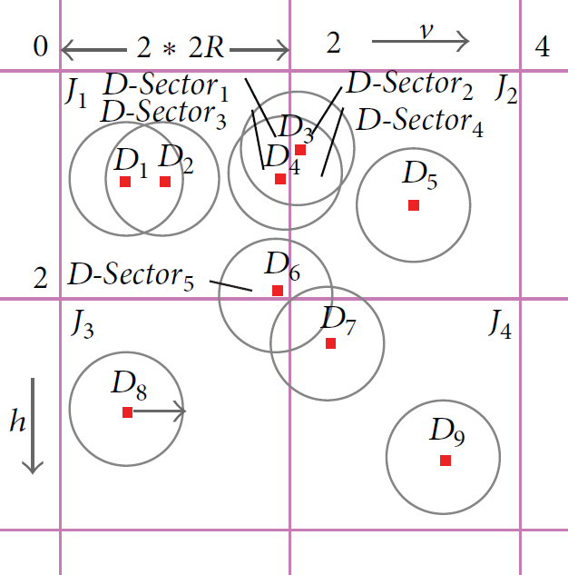
Grid subdivisions of $\mathrm{S}\mathrm{G}(\mathrm{0,0})\hspace{0.17em}\hspace{0.17em}(k=\mathrm{2},v=\mathrm{0},\hspace{0.17em}\hspace{0.17em}\mathrm{a}\mathrm{n}\mathrm{d}\hspace{0.17em}\hspace{0.17em}h=\mathrm{0})$ .

To obtain the needed optimum solution, several times of subgrid division are needed. When the value of k is given, the values of v and h are on the interval of $[\mathrm{0},k-\mathrm{1}]$ and there are $k\times k$ possibilities. $\mathrm{O}\mathrm{P}\mathrm{T}(v,h)$ denotes the optimum solution when the value of $v,h$ is fixed and the subgrid is divided. Then, there are $k\times k$ optimum solutions and the smallest solution of all the optimum solutions is the final solution, ${\mathrm{O}\mathrm{P}\mathrm{T}}^{\prime }(v,h)$ . Then, ${\mathrm{O}\mathrm{P}\mathrm{T}}^{\prime }(\nu ,h)=\mathrm{m}\mathrm{i}\mathrm{n}(\mathrm{O}\mathrm{P}\mathrm{T}(\nu ,h))\hspace{0.17em}\hspace{0.17em}(\mathrm{0}\le \nu ,h\prec k)$ .

This optimum solution is the minimum coverage solution in the circular region. After converting the circular region into the corresponding nodes, the current set of circular regions is converted into the corresponding set of nodes, that is, $S^{\mathrm{m}\mathrm{i}\mathrm{n}}$ , and a position of corresponding node in $S^{\mathrm{m}\mathrm{i}\mathrm{n}}$ will be an anchor point for UAV. Thus, the mission of finding the minimum coverage for aerial data collection is accomplished.

3.3.2. The Minimum Spanning Circle Algorithm

Algorithm 2 depicts the obtaining of the minimum coverage in one grid. This algorithm considers the nonempty square J as the input after calculating and outputting the minimum coverage $D_J$ of square J. In this algorithm, define set U as the collection of $D\text{-}Sector$ in J and now U contains all the elements in J. That is, U absolutely covers J. Count is the number of elements in the solution. U is the initial solution; then, the initial value of Count is the number of elements in U. Cyclically reduce the number of $D\text{-}Sector$ elements in U until the $D\text{-}Sector$ in U covers all the nodes in J and the number of $D\text{-}Sector$ cannot be reduced anymore. Then, U is the solution.

Algorithm 2: CALCOVER.

Input: An cover area of circular region J;

Output: Minimum cover of this region $D_J$ ;

(1) Initialize set $D_J(v,h)$ as all elements in J;

(2) Initialize Count as the size of $D_J(v,h)$ ;

(3) while Count decreased by 1 after every loop do

(4)   if all of the combination of the left D-Sector can't

   cover all elements then

(5)    $D_J=U$ ;

(6)   return   $D_J$ ;

(7)  else

(8)   Set U as the current combination;

(9)  end if

(10) end while

Algorithm 3 cites Algorithm 2. The main task of this algorithm is to accomplish the grid division of the whole region. And then use Algorithm 2 to calculate the minimum coverage of every nonempty square after the set of squares is obtained through division and combine all the minimum coverage of every square into global minimum coverage. Now, the grid still needs multiple times of division and each time global minimum coverage is obtained. In the end, the global minimum coverage containing the least nodes is the final solution. The key point of the algorithm is to obtain the nonempty square set $G(v,h)$ for every group of $v,h$ and to call Algorithm 2 for every J in $G(v,h)$ to calculate the minimum coverage solution $M_J(v,h)$ for all the circular region set $D_J(v,h)$ in J. After the division of the grid, combine all $M_J(v,h)$ and remove the overlapped areas and leave the global minimum coverage $M(v,h)$ of this grid division. Because there are errors in the minimum circle spanning during the grid division, first save the fixed value $M(v,h)$ to the result set $\mathrm{O}\mathrm{P}\mathrm{T}$ . When all the global minimum coverage of all combinations of $v,h$ is accomplished, take the global minimum coverage in the $\mathrm{O}\mathrm{P}\mathrm{T}$ which has the least circular regions as the final solution.

Algorithm 3: MINCOVER.

Input:  k;

Output:  A series of points represent the final solution $S^{\mathrm{m}\mathrm{i}\mathrm{n}}$ ;

(1) for   $v=\mathrm{0}$ ; $v<k$ ; v++  do

(2)  for   $h=\mathrm{0}$ ; $h<k$ ; h++   do

(3)   Calculate the non-empty sub-grid set $G(v,h)$ ;

(4)   for every element in $G(v,h)$   do

(5)    Calculate the minimum cover set

      $M_J(v,h)=\text{MINCOVER}(J)$ ;

(6)    Merge $M_J(v,h)$ into global mininum cover

      $M_J\left(v,h\right)=\bigcup _{J\in G\left(v,h\right)}^{}{M}_J(v,h)$ ;

(7)   end for

(8)   Add $G(v,h)$ which was achieved by this division into resolution set OPT;

(9)  end for

(10) end for

(11) For all elements in P calculate the cover which has minimum number of circle as the final resolution $S^{\min }$

(12) return   $S^{\min }$

3.4. The Path Planning of Aerial Vehicles

Nodes in $S^{\mathrm{m}\mathrm{i}\mathrm{n}}$ can be used as the anchor points for the UAV data collection. These nodes are called head nodes. The substance of the UAV path planning is to build an optimum path based on $S^{\mathrm{m}\mathrm{i}\mathrm{n}}$ that could visit all the head nodes. The process of visiting all the nodes from the starting point to the ending point can be considered as a classic Traveling Salesman Problem (TSP). TSP is an NP-Hard problem. To obtain the path of aerial vehicles faster, this paper proposes a FPPWR algorithm. Considering the notion that the network is a large-scale one and the deployment of nodes is well-distributed, this paper cites the grid division method described in Section 3.3.1 and divides the path planning of the global region into squares and then combines the paths in the squares based on the line precedence principle—that is, square in the same line precedes others when scanning.

Figure 1(d) shows the key step of path planning of the aerial vehicle. Figure 1(d) shows the grid division during calculation and the global regional path W for aerial vehicles obtained through fast path planning algorithm. The fast path planning algorithm will be elaborated in Section 4.

3.5. Data Collection

Figure 1(e) depicts the flow chart and schematic of the ground data collection separately. When the nodes in the network finish self-positioning, they disconnect the link and enter low power mode—the wireless module enters the dormant state and the sensor module starts to collect data. The sensor nodes store the data in their own storage space with limited capacity after data collection is finished. After a certain period of time, the aerial vehicle enters the network following a scheduled path and connects with the ground nodes to determine the position of data collection and starts to collect data from the sensor nodes that are in the coverage of the signal. Considering energy saving, the sensor nodes upload data through one-hop routing.

4. FPPWR for Aerial Data Collection

The process of aerial data collection can be briefed as follows. In a series of target locations, the mobile data collector needs to find the path that costs the least, visit the target locations for only once, and return to starting point. This problem can be abstracted as the TSP problem. And how to visit the target location at the least cost is the key of solving this problem. Now, the study of TSP problem can be categorized into the following five methods. First is the dynamic programming. Second is the greedy algorithm. Third is the branch definition method. Fourth is the backtracking method and fifth is the genetic algorithm. These methods could find solutions to the TSP problem, but they have a high time complexity and are easy to plunge into local optima.

When the sensor network has large amount of target nodes, it is time consuming to use the conventional methods to solve TSP and find the flight path of the aerial vehicle. And with the growth of scale, these conventional algorithms even may not find the final solutions to the problem. Besides, the flight path based on conventional methods of solving TSP has irregularity. And this kind of irregularity may easily cause the space discontinuity in data collection and is not good for the aerial data collection in a large-scale WSN. Specific to the above problems, this paper introduces the primary flight path and provides a feasible FPPWR algorithm for aerial data collection. This algorithm mainly utilizes grid division method in [20] and divides the global nodes into every subregion. Then, it combines the paths in the subregions through the primary flight path and finally obtains a global flight path quickly with certain regulations.

4.1. The Related Work of the UAV Path Planning

There are increasing interests in research works about the aerial data collection based on the controllable UAV. The basis of these studies is that the UAV can be controlled flexibly and will accomplish the flight mission following the scheduled flight plan. Lange et al. [23] stated a kind of high performance, controllable UAVs with multiaxis. This UAV can hover or land at the specific location with the help of GPS navigation system when it carries a certain degree of load.

The path planning for aerial data collection is to visit every target node at the lowest cost. In some application, cost can be represented by the Euclidean distance. In [18], sensor networks are often deployed in the large remote depopulated areas and the ground transportation is inconvenient. The authors let several UAVs work together and conducted path planning for the node set that each UAV is responsible for. The process of one UAV visiting nodes can be considered as a TSP. The authors used the greedy algorithm to find the shortest flight path. Although this algorithm can get the flight path fast, it often cannot find the optima. In [24], the authors used the branch definition method that is specific to TSP to solve the TSP. The branch definition method is one of the ways that could find exact solutions to the problem. However, this method is time consuming. When there are too many nodes, the method cannot find the final solution. Now, a better way to solve TSP is the Lin-Kernighan-Helsgaun algorithm [25]. The time complexity of the algorithm could reach $O(n^{\mathrm{2.2}})$ . To further reduce the time consumption of LKH algorithm, in [26, 27], the authors proposed modified algorithm based on generalized TSP. LKH algorithm is an algorithm with the lowest time complexity to solve the TSP. However, it has two shortcomings. Firstly, it may not find the optimum solution with one time of heuristic research. It might need several rounds to find the optimum solution, which can be more time consuming. Secondly, when the scale of problem increases, its time consumption will have $O(n^{\mathrm{2.2}})$ growth.

For those sensor networks whose nodes are well-distributed, the path planning of the nodes can be considered as an exception of TSP. In the meantime, considering that the deployment of sensor network is large scale, using grid division could ensure the high accuracy of path planning and considerably reduce the time consumption.

4.2. Models and Definitions

For the large-scale sensor network which is deployed in the monitored environment, S denotes the set of all the sensor nodes. For each functioning node, there is wireless signal coverage on its surrounding environment. In the connected sensor network, nodes can communicate mutually through wireless signal; as a consequence, there must be large scale of overlapping. $G^{\mathrm{o}\mathrm{p}\mathrm{t}}$ denotes the optimal solution of grid division through the minimal coverage algorithm, while $S^{\mathrm{o}\mathrm{p}\mathrm{t}}$ denotes the sensor node set from the optimal solution. Here, grid and square are involved, which can be denoted by G and J separately. In grid G, the sector divided by two adjacent horizontal lines is denoted by $\mathrm{R}\mathrm{w}$ . The sector divided by two adjacent vertical lines is denoted by $\mathrm{C}\mathrm{l}$ , and the quadrate intersection formed by $\mathrm{R}\mathrm{w}$ and $\mathrm{C}\mathrm{l}$ is square section. So, the scale of grid can be denoted by $\mathrm{R}\mathrm{w}\times \mathrm{C}\mathrm{l}\hspace{0.17em}\hspace{0.17em}(\mathrm{R}\mathrm{w}>\mathrm{0},\mathrm{C}\mathrm{l}>\mathrm{0})$ . Figure 5 shows the scale of a grid of $\mathrm{2}\times \mathrm{2}$ ; hereinto, $G^{\mathrm{o}\mathrm{p}\mathrm{t}}=\{J_{\mathrm{1}},J_{\mathrm{2}},J_{\mathrm{3}},J_{\mathrm{4}}\}$ .

Figure 5

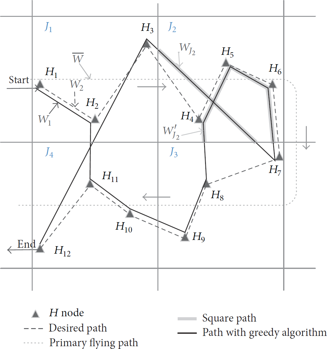
Path planning in the grid where there exist 12 H nodes.

Head node is a node that can gather date in its own coverage in the sensor network, denoted by H. Nodes in $S^{\mathrm{o}\mathrm{p}\mathrm{t}}$ are the minimum coverage solution in the network, so all the nodes in $S^{\mathrm{o}\mathrm{p}\mathrm{t}}$ are H nodes.

Flight path is a path based on the H node, seeking a path from the origin node to the end node to access all intermediary nodes, denoted by W.

The primary flight path is a path which can access the directed path of all intermediary squares from the origin square to the end square.

Ideal path is a kind of flight path with certain volatility and following the primary flight path.

Square path, also called local path, means the flight path W that is divided into square during grid division. $W_J$ denotes the flight path of square J.

FPPWR is the flight path formed by all the grid paths that have a unique directed path.

Ingress node is the first H node in square J accessed by directed square path $W_J$ , denoted by $H^{\mathrm{i}\mathrm{n}}$ .

Out node is the last H node in square J accessed by directed square path $W_J$ , denoted by $H^{\mathrm{o}\mathrm{u}\mathrm{t}}$ .

As is shown in Figure 5, it is a schematic of the grid division and flight path of 12 H nodes. The greedy path $W_{\mathrm{1}}$ is a flight path originated with $H_{\mathrm{1}}$ node and ended by $H_{\mathrm{12}}$ node, seeking the nearest node as its next traversal node under the guidance of greedy algorithm. In square $J_{\mathrm{2}}$ , the present square is formed by polygonal lines $W_{J_{\mathrm{2}}}$ and $W_{J_{\mathrm{2}}}^{\prime }$ , so $W_{\mathrm{1}}$ is an irregular path. $\bar{W}$ is a primary flight path (denoted by imaginary line); it enters $J_{\mathrm{1}}$ , through $J_{\mathrm{2}}$ and $J_{\mathrm{3}}$ , and exits from $J_{\mathrm{4}}$ . However, $W_{\mathrm{2}}$ is a regularized path with certain volatility along the primary flight path. Based on $W_{\mathrm{2}}$ , it is possible to find that in square $J_{\mathrm{1}}$ node $H_{\mathrm{1}}$ is the ingress node and node $H_{\mathrm{3}}$ is the out node.

The reason for the existence of irregular path is the repetition access of square in the path planning process, which causes the same square to be accessed at least for one time. In order to avoid the existence of the irregular path and find the regularized path, we need to plan the access of square with certain sequence. The process can be summarized as the projecting of primary flight path. In order to achieve the sequential square set $G^{\mathrm{s}\mathrm{o}\mathrm{r}\mathrm{t}}$ , the primary flight path needs to be planned according to the line precedence principle. Line precedence means, when planning the path of aircraft, squares in the same line have the priority to be the next access square until the paths of all squares have been projected. As imaginary line $\bar{W}$ shown in Figure 5, the path enters the grid at $\mathrm{R}{\mathrm{w}}_{\mathrm{1}}$ , then accesses $J_{\mathrm{1}}$ , the first square of the line, and accesses $J_{\mathrm{2}}$ and $J_{\mathrm{3}}$ in the guidance of line precedence principle; finally, it exits the grid at $J_{\mathrm{4}}$ . So, $G^{\mathrm{s}\mathrm{o}\mathrm{r}\mathrm{t}}=\left\{J_{\mathrm{1}},J_{\mathrm{2}},J_{\mathrm{3}},J_{\mathrm{4}}\right\}$ .

Considering the complexity and efficiency of an algorithm, to obtain an ideal regular path, the whole path can be divided into paths in the local squares. And combine all the paths in the local squares in the primary flight path to obtain a whole path. $S^{\mathrm{s}\mathrm{o}\mathrm{r}\mathrm{t}}$ denotes the whole path, and $S_J^{\mathrm{s}\mathrm{o}\mathrm{r}\mathrm{t}}$ denotes the flight path of square J. So, we can work out the formula of path planning:

$$\begin{array}{cc}& S^{\mathrm{s}\mathrm{o}\mathrm{r}\mathrm{t}}={\displaystyle \bigcup }_{J\in G^{\mathrm{s}\mathrm{o}\mathrm{r}\mathrm{t}}}{S}_J^{\mathrm{s}\mathrm{o}\mathrm{r}\mathrm{t}}.\end{array}$$

(1)

From the formula above, the main workload of UAV is square traversal and path planning, and the function of primary flight path is to regularize the path planning. After the path is planned, a sequential node set $S^{\mathrm{s}\mathrm{o}\mathrm{r}\mathrm{t}}$ which concludes all H nodes in $S^{\mathrm{o}\mathrm{p}\mathrm{t}}$ will be obtained. And the sequence of H node in $S^{\mathrm{o}\mathrm{p}\mathrm{t}}$ decides the access sequence of H node in the monitored environment. The details would be narrated in Section 4.3.

4.3. UAV Regularized Fast Path Planning

In this section, the paper describes in detail how to plan the path of square and optimize the whole path, based on primary flight path. Square path planning is a kind of local path planning; there are small quantity node sets in each square, so the path planning would be efficient, which would be narrated in Section 4.3.1 for the path planning of a single square; ingress node and out node must be taken into consideration. To ensure the ingress node and out node of a square, the concept of operator is introduced, and optimal algorithm of path based on paired operators is raised. Details are shown in Section 4.3.2.

Primary flight path is a conceptual directed path, which clarified the access sequence. From the detailed path planning of a square and the optimizing of paired operators, a sequential node set including all the nodes to be accessed can be obtained. Connecting all these nodes by sequence, a directed path would be formed and that is the UAV flight path.

4.3.1. Paths in Square Areas

Because of the random nodes distribution, there could be some empty squares which would be ignored in the path planning. Based on the precedence principle, the other squares can obtain the sequential nonempty square set $G_{\mathrm{s}\mathrm{o}\mathrm{r}\mathrm{t}}$ in the primary flight path.

With the division of grid, node set $S_{\mathrm{o}\mathrm{p}\mathrm{t}}$ would be decentralized into each nonempty square $J\hspace{0.17em}\hspace{0.17em}(J\in G_{\mathrm{s}\mathrm{o}\mathrm{r}\mathrm{t}})$ . $S_J$ denotes the node set of square J, so $S_J\subseteq S_{\mathrm{o}\mathrm{p}\mathrm{t}}$ . In J, path-ordering is the local square path drawn by quick sorting algorithm and ordered in the primary flying direction of $S_J$ , and the corresponding sequential node set is denoted by $S_{J\mathrm{s}\mathrm{o}\mathrm{r}\mathrm{t}}$ .

Although $S_{J\mathrm{s}\mathrm{o}\mathrm{r}\mathrm{t}}$ concludes all nodes in J, for the whole path, $H_{\mathrm{o}\mathrm{u}\mathrm{t}}$ and $H_{\mathrm{i}\mathrm{n}}$ in J are still not ideal. So, after obtaining $S_{J\mathrm{s}\mathrm{o}\mathrm{r}\mathrm{t}}$ , paired operators path optimization algorithm (Algorithm 5) would be transferred to determine the ingress node and out node of the square. Algorithm 4 has described the process of the square path planning and the whole path planning. This algorithm focuses on the traversal of square (Line (3) to Line (8)). During the loop operation, a square is chosen each time. By quick sorting algorithm, all H nodes in the present square J would be sorted in the primary flight path; then, Algorithm 5 is transferred. After Algorithm 5, it is possible to find that the ingress node and out node of a square are modified. So, the returned value can be merged into the whole path $S_{\mathrm{s}\mathrm{o}\mathrm{r}\mathrm{t}}$ .

Algorithm 4: SquarePlan.

Input:   $G^{\text{opt}}$ : The optimal grid; $S^{\text{opt}}$ : The set of the positioned nodes;

Output:   $S^{\text{sort}}$ : An ordered set of the nodes;

(1) Set $G^{\text{sort}}$ as the result of sorting $G^{\text{opt}}$   using primary flight path;

(2) Set $J_{\text{pre}}=null$ ;

(3) for  square J in $G^{\text{sort}}$   do

(4)  Set $S_J^{\text{sort}}$ as the result of sorting $S_J$ with quick sort method;

(5)  Set $S_{J_{\text{pre}}}^{\text{sort}}$ = Call IOPlan( $J_{\text{pre}},J$ );

(6)   $S^{\text{sort}}=S^{\text{sort}}\cup S_{J_{\text{pre}}}^{\text{sort}}$ ;

(7)   $J_{\text{pre}}=J$ ;

(8) end for

(9) return   $S^{\mathrm{s}\mathrm{o}\mathrm{r}\mathrm{t}}$

Algorithm 5: IOPlan.

Input: $J_{\mathrm{p}\mathrm{r}\mathrm{e}}$ : Previous square; J: Current square;

Output: $S_{\mathrm{s}\mathrm{o}\mathrm{r}\mathrm{t}}$ : The set to store output result;

Variable:

$P_{\mathrm{p}\mathrm{r}\mathrm{e}},P$ : Suspicious set;

η: The size of suspicious set;

$H_{\mathrm{i}\mathrm{n}}$ , $H_{\mathrm{o}\mathrm{u}\mathrm{t}}$ : The leaving node and the entrance node;

R: Enum values representing the relationship $J_{\mathrm{p}\mathrm{r}\mathrm{e}}$ and J;

Initialize:

R with the relationship of J and $J_{\mathrm{p}\mathrm{r}\mathrm{e}}$ ;

P with the last η nodes from J;

$P_{\mathrm{p}\mathrm{r}\mathrm{e}}$ with the top η nodes from $J_{\mathrm{p}\mathrm{r}\mathrm{e}}$

 (1) Manipulation Data

  switch  R  do

   case  Case  LEFT-RIGHT

   Paired Operator: Find $H_{\mathrm{i}\mathrm{n}}$ and $H_{\mathrm{o}\mathrm{u}\mathrm{t}}$ with

   exhaustive method;

   break;

   case  UP-DOWN

   Paired Operator: Find the node with max vertical

   projection in P as $H_{\mathrm{i}\mathrm{n}}$ , and find the node with

   min vertical projection in $P_{\mathrm{p}\mathrm{r}\mathrm{e}}$ as $H_{\mathrm{o}\mathrm{u}\mathrm{t}}$ ;

   break;

   case  START-EDN

   Paired Operator: No operation;

   endsw

 (2) Adjust $H_{\mathrm{i}\mathrm{n}}$ to the top position in J, and $H_{\mathrm{o}\mathrm{u}\mathrm{t}}$ to the last position in $J_{\mathrm{p}\mathrm{r}\mathrm{e}}$ ;

 (3) Copy the sorted head nodes in $J_{\mathrm{p}\mathrm{r}\mathrm{e}}$ to $S_{\mathrm{s}\mathrm{o}\mathrm{r}\mathrm{t}}$ ;

 (4) return   $S_{\mathrm{s}\mathrm{o}\mathrm{r}\mathrm{t}}$ ;

4.3.2. Optimum of the Paired Operators' Path

To optimize the distance from the present square to the next square, the concept of operator is introduced to determine the ingress node and out node of a square. The operator seeking the ingress node is defined as ingress operator denoted by $\mathrm{f}\mathrm{i}\mathrm{n}\mathrm{d}\mathrm{I}\mathrm{n}$ ; the operator seeking the out node is defined as the out operator denoted by $\mathrm{f}\mathrm{i}\mathrm{n}\mathrm{d}\mathrm{O}\mathrm{u}\mathrm{t}$ . Suspicious set is the node set while working out the ingress node, which is denoted by P. The number of nodes in the suspicious set is defined as the capacity of a suspicious set defined by η. Ingress node and its nearby nodes form a suspicious set, defined as ingress suspicious set denoted by $P^{\mathrm{i}\mathrm{n}}$ . Out node and its nearby node formed a suspicious set, defined as out suspicious set denoted by $P^{\mathrm{o}\mathrm{u}\mathrm{t}}$ . Thereby, the process of seeking ingress node is the process of $\mathrm{f}\mathrm{i}\mathrm{n}\mathrm{d}\mathrm{I}\mathrm{n}$ seeking ingress node in $P^{\mathrm{i}\mathrm{n}}$ , and the process of seeking out node is the process of $\mathrm{f}\mathrm{i}\mathrm{n}\mathrm{d}\mathrm{I}\mathrm{n}$ seeking out node in $P^{\mathrm{o}\mathrm{u}\mathrm{t}}$ .

$L(H,H^{\prime })$ is the flight path distance from node H to node $H^{\prime }$ . When $H\in S_J,H^{\prime }\in S_{J^{\prime }}$ , and the flight path is from J to $J^{\prime }$ , $L(H,H^{\prime })$ represents the flying distance from the present square to the next one. If $L^{\mathrm{m}\mathrm{i}\mathrm{n}}(H,H^{\prime })$ represents the minimal distance, node H is the node $H^{\mathrm{o}\mathrm{u}\mathrm{t}}$ sought by $\mathrm{f}\mathrm{i}\mathrm{n}\mathrm{d}\mathrm{O}\mathrm{u}\mathrm{t}$ . So, the process of $\mathrm{f}\mathrm{i}\mathrm{n}\mathrm{d}\mathrm{I}\mathrm{n}$ and $\mathrm{f}\mathrm{i}\mathrm{n}\mathrm{d}\mathrm{O}\mathrm{u}\mathrm{t}$ seeking ingress node and out node should be collaboratively operated with the $\mathrm{f}\mathrm{i}\mathrm{n}\mathrm{d}\mathrm{O}\mathrm{u}\mathrm{t}$ of the present square and the $\mathrm{f}\mathrm{i}\mathrm{n}\mathrm{d}\mathrm{I}\mathrm{n}$ of the next square to determine the ingress node and out node of a square. $J_{\mathrm{f}\mathrm{i}\mathrm{n}\mathrm{d}\mathrm{O}\mathrm{u}\mathrm{t}}$ denotes the out operator of the present square, and $J_{\mathrm{f}\mathrm{i}\mathrm{n}\mathrm{d}\mathrm{I}\mathrm{n}}^{\prime }$ denotes the ingress operator of the present square, so the combination of $J_{\mathrm{f}\mathrm{i}\mathrm{n}\mathrm{d}\mathrm{O}\mathrm{u}\mathrm{t}}$ and $J_{\mathrm{f}\mathrm{i}\mathrm{n}\mathrm{d}\mathrm{I}\mathrm{n}}^{\prime }$ is called paired operators, and $P_J^{\mathrm{o}\mathrm{u}\mathrm{t}}$ in corresponding square J and $P_{J^{\prime }}^{\mathrm{i}\mathrm{n}}$ in J is paired suspicious set.

The key point of paired operators seeking ingress and out node is to choose the right seeking way while guaranteeing the minimal distance when entering into the next square from the present square and improve the efficiency of the algorithm. Aimed at the position of suspicious set, the following will explain the seeking method of corresponding paired operators.

START-END is the suspicious set including ingress node and out node when the aircraft enters and exits from the whole area. In the whole area, entrance and exit mean the beginning and end of data collection, so there would be two suspicious sets: $P^{\mathrm{s}\mathrm{t}\mathrm{a}\mathrm{r}\mathrm{t}}$ denotes the one at the beginning and $P^{\mathrm{e}\mathrm{n}\mathrm{d}}$ denotes the one in the end. Lacking directly connected square, $\mathrm{f}\mathrm{i}\mathrm{n}\mathrm{d}\mathrm{I}\mathrm{n}$ and $\mathrm{f}\mathrm{i}\mathrm{n}\mathrm{d}\mathrm{O}\mathrm{u}\mathrm{t}$ would see the node nearest boundary as the ingress and out node. As shown in Figure 6, the grid includes the sketch of $P^{\mathrm{s}\mathrm{t}\mathrm{a}\mathrm{r}\mathrm{t}}$ and $P^{\mathrm{e}\mathrm{n}\mathrm{d}}$ , and $\mathrm{f}\mathrm{i}\mathrm{n}\mathrm{d}\mathrm{I}\mathrm{n}$ chooses $H_{\mathrm{1}}$ as the ingress node while $\mathrm{f}\mathrm{i}\mathrm{n}\mathrm{d}\mathrm{O}\mathrm{u}\mathrm{t}$ chooses $H_{\mathrm{47}}$ as the out node.

Figure 6

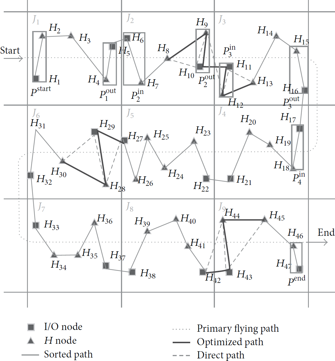
Workflow of FPPWR.

UP-DOWN is the paired suspicious set made up of two suspicious sets when the aircraft leaves for another line from the present line. If the present square is J, and the next line to be accessed is $J^{\prime }$ , $P_J^{\mathrm{o}\mathrm{u}\mathrm{t}}$ and $P_{J^{\prime }}^{\mathrm{i}\mathrm{n}}$ formed a paired suspicious set. The paired operators would sort nodes in $P_J^{\mathrm{o}\mathrm{u}\mathrm{t}}$ and $P_{J^{\prime }}^{\mathrm{i}\mathrm{n}}$ in the vertical direction and choose the bottom node in $P_J^{\mathrm{o}\mathrm{u}\mathrm{t}}$ as the out node of J and the top node in $P_{J^{\prime }}^{\mathrm{i}\mathrm{n}}$ as the ingress node of $J^{\prime }$ . As shown in Figure 6, the suspicious set made by $P_{\mathrm{3}}^{\mathrm{o}\mathrm{u}\mathrm{t}}$ and $P_{\mathrm{4}}^{\mathrm{i}\mathrm{n}}$ is up-down suspicious set. $\mathrm{f}\mathrm{i}\mathrm{n}\mathrm{d}\mathrm{O}\mathrm{u}\mathrm{t}$ chooses $H_{\mathrm{16}}$ in $P_{\mathrm{3}}^{\mathrm{o}\mathrm{u}\mathrm{t}}$ as the out node. $\mathrm{f}\mathrm{i}\mathrm{n}\mathrm{d}\mathrm{I}\mathrm{n}$ chooses $H_{\mathrm{17}}$ in $P_{\mathrm{4}}^{\mathrm{i}\mathrm{n}}$ as the ingress node.

LEFT-RIGHT is the paired suspicious set made up of two suspicious sets when the aircraft moves from one square to the next square. In the function of paired operators, if the aircraft is from J to $J^{\prime }$ , the operator would choose the combination of nodes to make $L(H,H^{\prime })\hspace{0.17em}\hspace{0.17em}(H\in P_J^{\mathrm{r}\mathrm{i}\mathrm{g}\mathrm{h}\mathrm{t}},H^{\prime }\in P_{J^{\prime }}^{\mathrm{l}\mathrm{e}\mathrm{f}\mathrm{t}})$ get the minimal value. $\mathrm{f}\mathrm{i}\mathrm{n}\mathrm{d}\mathrm{O}\mathrm{u}\mathrm{t}$ chooses H as the out node of J. $\mathrm{f}\mathrm{i}\mathrm{n}\mathrm{d}\mathrm{I}\mathrm{n}$ chooses $H^{\prime }$ as the ingress node of $J^{\prime }$ . As shown in Figure 6, $P_{\mathrm{2}}^{\mathrm{o}\mathrm{u}\mathrm{t}}$ and $P_{\mathrm{3}}^{\mathrm{i}\mathrm{n}}$ form the left-right paired suspicious set. Paired operators choose $H_{\mathrm{10}}$ as the out node of J and $H_{\mathrm{11}}$ as the ingress node of $J^{\prime }$ .

After the out and ingress node of square J are determined, the ingress node would be modulated to the head of $S_J^{\mathrm{s}\mathrm{o}\mathrm{r}\mathrm{t}}$ and the out node to the rear of $S_J^{\mathrm{s}\mathrm{o}\mathrm{r}\mathrm{t}}$ , by which the path of a square is optimized.

4.4. Description of Optimized Path Algorithm of Paired Operators

The operator seeking the ingress node is defined as the ingress operator. The operator seeking the out node is defined as the out operator. Suspicious set is the node set which works out the ingress node denoted by P. The number of nodes in the suspicious set is defined as the capacity of a suspicious set which is defined by η. The ingress node and its nearby nodes form a suspicious set, defined as the ingress suspicious set denoted by $P^{\mathrm{i}\mathrm{n}}$ . Out node and its nearby nodes form a suspicious set, defined as the out suspicious set denoted by $P^{\mathrm{o}\mathrm{u}\mathrm{t}}$ . Thereby, the process of seeking ingress nodes is the process of ingress operator seeking ingress node in $P^{\mathrm{i}\mathrm{n}}$ , and the process of seeking out node is the process of out operator seeking out node in $P^{\mathrm{o}\mathrm{u}\mathrm{t}}$ .

To find the minimal distance from the present square to the next square, out operator and ingress operator need to operate collaboratively to determine the out node and the ingress node. The two operators are called paired operators, and the corresponding out suspicious set and ingress suspicious set are called paired suspicious set.

The key point of paired operators seeking the ingress and the out node is choosing the right seeking way while guaranteeing the minimal distance when entering into the next square from the present square and improving the efficiency of the algorithm. The paired suspicious set, in accordance with the position of out suspicious set and ingress suspicious set, can be divided into three types, START-END, UP-DOWN, and LEFT-RIGHT. As shown in Figure 6, it is an optimized process of paired operators in a suspicious set capacity of 2 and the grid scale of $\mathrm{3}\times \mathrm{3}$ . The detailed algorithm is presented in Algorithm 5.

4.5. Analysis of the Algorithm Complexity

From Algorithm 1, the traversal of all squares and the sort of nodes in every access square are the two main loop parts in this algorithm. For the sort of nodes in a square, we apply the quick sort algorithm which needs lower time complexity to achieve the sequential node set along the primary flying path. According to the quick sorting algorithm, when s nodes participate in sort, the time complexity is

$$\begin{array}{cc}& O\left(s\right)=s\mathrm{l}\mathrm{o}{\mathrm{g}}_{\mathrm{2}}s.\end{array}$$

(2) So, if $G^{\mathrm{o}\mathrm{p}\mathrm{t}}$ concludes m squares, and all the squares need to conduct quick sort, the time complexity is

$$\begin{array}{cc}& O\left(m\right)={\displaystyle \sum }_{i=\mathrm{1}}^m{s}_i\mathrm{l}\mathrm{o}{\mathrm{g}}_{\mathrm{2}}{s}_i.\end{array}$$

(3) The sensor network is deployed evenly, so the number of nodes is roughly alike. If the general number of H nodes is n, the original formula can be evolved into

$$\begin{array}{cc}& O\left(m\right)=ms\mathrm{l}\mathrm{o}{\mathrm{g}}_{\mathrm{2}}s,\\ n=ms.\end{array}$$

(4) Derivation is as follows:

$$\begin{array}{cc}& O\left(n\right)=n\mathrm{l}\mathrm{o}{\mathrm{g}}_{\mathrm{2}}s\hspace{1em}\left(\mathrm{1}\le s\le n\right).\end{array}$$

(5) For a sensor network having n nodes, the time complexity of FPPWR is $O(n)=n\mathrm{l}\mathrm{o}{\mathrm{g}}_{\mathrm{2}}s$ . This shows that the sparser the division of grid $G^{\mathrm{o}\mathrm{p}\mathrm{t}}$ , the more the sorting work to be done. When $s=\mathrm{1}$ , each square has one node, and the flight path is the primary flight path; when $s=n$ , $G^{\mathrm{o}\mathrm{p}\mathrm{t}}$ only contains one square, and FPPWR algorithm evolves into a quick sorting algorithm.

4.6. The Result of the Experiment and Its Analysis

Based on Windows operating system, FPPWR sorting algorithm is realized by C# language. The processor is Core i5 dual core, 2.4 GHz. Since this algorithm is focused on projecting large numbers of nodes, as for the node and its input, we can use the function $(\mathrm{R}\mathrm{a}\mathrm{n}\mathrm{d}\mathrm{o}\mathrm{m}())$ which is characterized by uniform distribution to generate available node. As for the time consumption of the algorithm, we can use Stopwatch which is a timer from C# language Software Development Kit (SDK), combined with other functions related to TimeSpan, to calculate the time consumed by algorithm precisely. As for the path distance, the practical distance and distance between nodes could be resized with certain rate on the computer screen and shown by pixel distance. Uniform distribution is the ideal situation. In order to reduce the chance caused by the random function, we do multiple experiments on different number of nodes until the result is stable. After getting the statistics of time consumption of LKH, greedy, and FPPWR algorithms, the contrast of the three algorithms can be made. The following is the list of necessary parameters and their explanation.

Table 1 describes the necessary parameter in the experiment, among which the scale of grid decides the number of the squares, generates certain scale of grid, and gets the grid division in minimal covering. The number of nodes decides the number of head nodes in each square. The number of head nodes combined with the grid number parameter can describe the deployment scale of the sensor network. The size of operator decides the number of nodes included in each operator in the experiment, which provides the limitation for suspicious set capacity in the optimized algorithm of the operator path. Figure 7 shows the result of path planning.

Table 1

Algorithm parameters of the FPPWR.

Name	Type	Node
Grid scale	Integer	The size of the grid
Sensors	Integer	The number of sensor nodes in one square
Operator size	Integer	The size of the operator for path optimization

Figure 7

Experimental result of FPPWR under conditions grid scale: $\mathrm{8}\times \mathrm{6}$ .

To highlight the advantage of the FPPWR algorithm, we conduct 13 experiments; the numbers of nodes are 100, 200, 300, 500, 1000, 1500, 2000, 3000, 5000, 10000, 20000, 30000, and 50000; and numbering the experiment is based on the different number of nodes. For each group experiment, besides the number of nodes, other conditions keep the same. The path, respectively, is projected by the FPPWR algorithm, greedy algorithm, and heuristic algorithm; the path distance and time consumption of the algorithm are collected. The following two parameters are used to analyze FPPWR algorithm performance: time consumption in path planning and path distance.

4.6.1. Analysis of Time Consumption

When planning the path in different node scale, time consumed by the FPPWR algorithm is various. From the number of nodes and the time consumed in path planning in Figure 6, we can conclude the relationship between time consumption and number of nodes, shown in Figure 8(a).

Figure 8

(a) Time consumption. (b) Uniform contrast. (c) Nonuniform contrast.

From the figure, it is possible to find that the fewer the nodes, the less the time consumption of FPPWR. When the number of nodes is less than 3000, the time consumed is less than 1 ms; when the number of nodes increases, the time consumption increases linearly.

By contrasting with LKH algorithm and greedy algorithm, the time consumption between them has a huge difference, as shown in Figure 8(a). From the figure, when the number of nodes is less than 3000, the time consumption of these three algorithms is less, while FPPWR algorithm is the least time consuming. When the number of nodes is more than 3000, the time consumption of these three algorithms begins to show a huge difference, and the time consumption of LKH is the largest. From the figure, when the number of nodes reached 50000, the time consumption of LKH is 957820.4 ms, which is about eighty thousand times bigger than the time consumption of FPPWR. The reason for this huge difference is that LKH algorithm and greedy algorithm search the solution accessing target nodes within the global scope, aiming at less path distance, while FPPWR divides the global scope into square area using grid and searches the solution with Row-prior principle. From the experiment, we can conclude that when there are a very large number of sensor nodes in the network, FPPWR algorithm is more advantageous in time consumption of computing the path planning.

4.6.2. Analysis of the Path Distance

Since the minimal path distance can be obtained through heuristic algorithm, the distance obtained through heuristic algorithm is regarded as datum which is used to compare with other distances obtained by other algorithms. After calculating its specific value, we can draw the path distance and node number chart as in Figure 8(b).

From the chart, it is possible to find that when the number of nodes is small, the short distance can be obtained from both heuristic algorithm and greedy algorithm. However, with the number of nodes increasing greatly, the FPPWR algorithm and the other two algorithms have the same effect.

In conclusion, when the number of nodes increases, the consumption of time increases greatly in greedy algorithm and heuristic algorithm. When the number reached 5000, the time consumed by heuristic algorithm is 10 times that of greedy algorithm and thousands of times that of the FPPWR algorithm. Meanwhile, as for the path distance, with the number of nodes increasing, the result of the FPPWR algorithm is close to that of the heuristic algorithm. So, if the path planning is not required to be too accurate, grid division has more advantages than other algorithms.

However, the FPPWR algorithm requires the node to be deployed evenly. For the unevenly deployed nodes, the feasible solution can be obtained through the algorithm but this solution has no advantage in finding the path distance. How the unevenly deployed nodes affect the FPPWR algorithm will be shown in the experiment.

4.7. The Effect of the Uneven Distribution to Algorithms

In this section, the paper focuses on the unevenly deployed sensor network and proves the efficiency of the FPPWR algorithm by experiments. In the experiment, the uneven deployment can be realized by deploying some empty squares. As is shown in the network deployment chart (Figure 8(b)), a flight path is obtained by the FPPWR algorithm. From this chart, it is possible to see, in such network deployment, the FPPWR algorithm cost 0.09 ms, and the path distance is 3029.94 pixels.

From Figure 9, it is possible to see that unevenly deployed nodes make the flight across several empty squares, and the flight distance is extended. In the circumstance of uneven deployment, we can have multigroup experiments of various numbers of nodes, based on the distance drawn by heuristic algorithm, the comparative chart of FPPWR algorithm, greedy algorithm, and heuristic algorithm, shown in Figure 8(c).

Figure 9

Experimental result of FPPWR with WSNs deployed nonuniformly.

From the data of experiment, path distance would be affected heavily citing the FPPWR algorithm when nodes are deployed unevenly: with the node number increased, the path distance deviation is larger in the FPPWR algorithm. So, in the unevenly deployed network, the FPPWR algorithm is ineffective.

5. Simulation Platform for Aerial Data Collection

For the sensor network deployed in large scale, there would be thousands of sensor nodes deployed in the monitored area. During data collection, the aircraft need to traverse all the grids with a sink node to accomplish the task of collecting all the node data. It is a time-consuming process, and the aircraft needs to bring enough fuel and enough storage space for data collection. So, how to precisely ensure that the amount of fuel, the storage space, and the length of time the aircraft needed are enough is significant. Based on this, this paper builds a simulation platform for aerial data collection based on collection steps.

5.1. Explanation for the Simulation Platform

The simulation platform can be divided into the simulation control program and the NS2 simulation routine. The simulation control program is developed by C# programming language in VS2005, which is focused on the allocation of relative data and the display of result. Besides, the following is also to be realized: the allocation of distributed nodes based on probability and the supporting algorithm related to simulation platform, such as Minimum Spanning Circle Method and the FPPWR. NS2 is developed by TCL script, which is mainly to realize the simulation of WSN in different deployment and output the result.

5.1.1. The Explanation of Basic Parameters

Table 2 shows the key parameters and notes in the simulation platform. All the parameters show the information of sensor network and nodes and deploy the corresponding simulation modules.

Table 2

Algorithm parameters of the FPPWR.

Name	Type	Node
Nodes	Integer	The number of sensor nodes in WSN
Deployment	Enumeration	The way of WSN deployment (manual, random, or with rules)
Coverage radius	Integer	The radius of the signal from sensors (meter)
Transmission rate	Float	The rate of the wireless communication (KB/s)
Acquisition rate	Integer	Sampling frequency (Byte/min)
UAV speed	Float	Speed of the UAV (m/s)
Sojourn time	Integer	The time staying on the top of the head nodes for collecting data (s)

5.1.2. The Effect of the Simulation Platform

The simulation platform is deployed according to the key parameters. Figure 10 shows the network coverage obtained when the network scale is 135 and the deployment is random and well-distributed.

Figure 10

The node coverage of simulation platform.

As is shown in Figure 10, simulation platform provides simulation network, minimal coverage, the path planning, and generation of NS2 script. Their functions are the following.

Simulation network: it generates needed sensor network according to the scale of the network and the deployment method, including ordinary nodes and movable sink nodes.

Minimal coverage: it uses the Minimum Spanning Circle Method to achieve the head nodes through transfer network, covering radius, and so forth.

Path planning: it cites the FPPWR algorithm to make quick path planning in accordance with the returned head nodes in minimal coverage.

Generation of NS2 script: it transfers the data collected by the aircraft and guided by FPPWR algorithm into TCL script and controls the simulation aircraft with sink node in NS2 WSN access node sequentially.

After the four processes, a TCL script would be generated in NS2. To achieve the simulation condition of aerial data collection in NS2, the experiment would track the parameters of received and transmitted data as well as the energy consumption and record the distance and time of the simulated aircraft. Figure 11 shows the simulation condition of sensor network in NS2 when the node scale is 135.

Figure 11

The simulation of network with NS2.

From Figure 11, when the time is 239.2 seconds, the sink node labeled 0 directly approaches the head node labeled 30 from the head node labeled 24 at a speed of 5 m/s. When moved to a head node, the sink node should stay for 20 seconds. Finally, at 1349.9, sink node stops moving, and the simulation network stops.

5.2. Analysis of the Simulation Experiment

After modifying the number of nodes and aircraft speed, respectively, multiple groups of experiments have been conducted, and the simulation results of each group's flight time, distance, and the collected data size are recorded. To express the simulation result of aerial data collection in NS2, the trends have been drawn to reflect the relationship between flight time, flight distance, and the size of collected data.

Figure 12, respectively, describes the relationship between consumed time during collection and the number of nodes. From the chart, with the increased number of nodes, the time consumed during collecting the data is correspondingly increased. Meanwhile, it is possible to find in the figure that the flight speed affects the time consumption greatly, especially when the large scale of node appears. And the increase of speed reduces the time consumption largely.

Figure 12

Relationship between time consumption and number of nodes.

Figure 13 is a relationship chart reflecting the change of flight distance of data collecting aircraft when the number of nodes changes. Since the flight distance is constant when the flight speed changed, the flight distance has no direct relationship with flight speed. And it is possible to find in the figure that the flight distance increases when the number of nodes increases. The detailed relationship has been narrated in the last part.

Figure 13

Relationship between the flight distance and the number of nodes.

Figure 14 is the trends reflecting how the amount of collected data changes when the number of nodes changes. From the chart, it is possible to find that when the number of nodes increases, the amount of data increases. When there are fewer nodes, the amount of data increases slowly. However, when the number of nodes increases, the amount of data increases greatly. The explanation for this phenomenon is that when the aircraft is collecting data, the node is also collecting data, and nodes near the end of the flight path can collect more data. Besides, the amount of collected data is related to flight speed: when the number of nodes keeps the same, the faster the aircraft flies, the less the data can be collected.

Figure 14

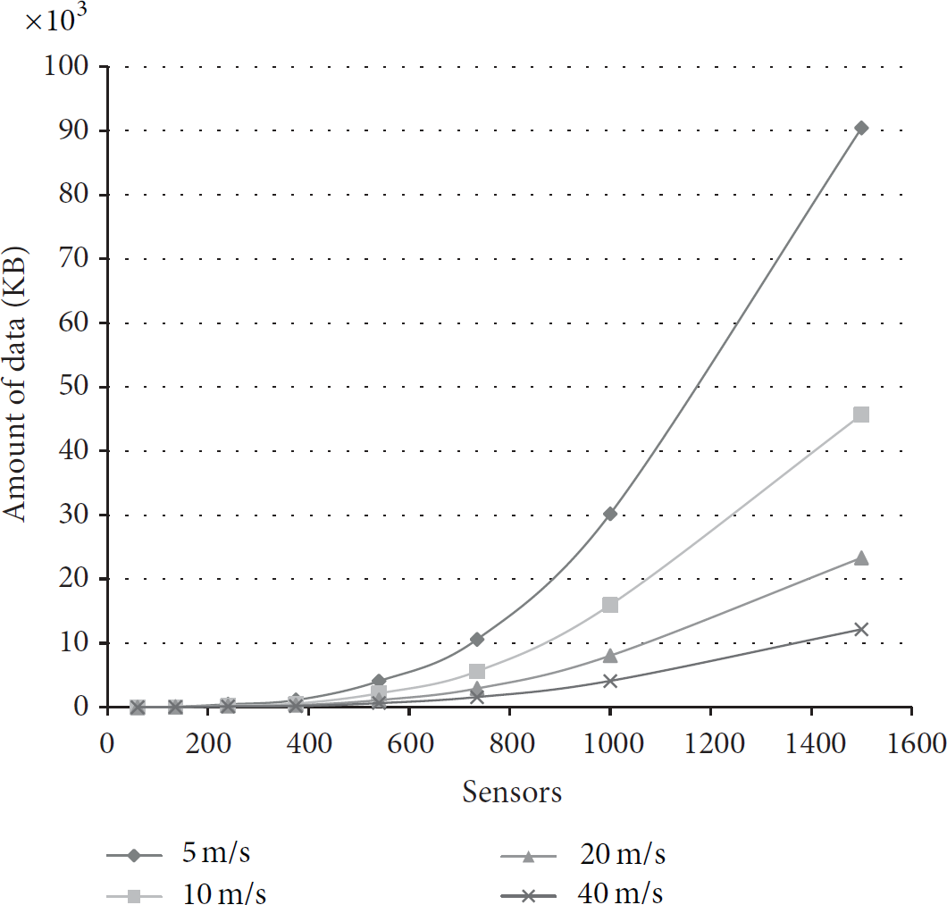
Relationship between the amount of data collected and the number of nodes.

Analyze comprehensively: from the simulation result of NS2, when the number of nodes increases and the flight speed remains the same, data collection costs more time, and flight distance and the amount of collected data increase, and the amount of collected data is larger than others. It is possible to find that when the number of nodes reaches 1500, the data collection of a sensor consumed 328.7 hours (13.7 days) and the flight distance is 28.2 km, and the amount of collected data reaches 90447 KB. So, from the simulation platform, a conclusion can be drawn that when the network deployment and parameter allocation are alike, the aircraft would at least fly 28.2 km and bring storage with the capacity of at least 90447 KB.

However, the speed of the aircraft affects a lot the time consumption, flight distance, and the amount of collected data. From the simulation result, the increase of speed would decrease the consumed time and the amount of collected data and improve the efficiency of data collection. These are also the advantages which are based on the aerial data collection based on UAV collecting data from a large-scale WSN.

6. Outlooks and Conclusions

Aimed at large-scale WSN, this paper studies a more practical method of aerial data collection. As for the construction of aerial data collection, it is divided into five procedures: deployment of network, allocation of distributed node, anchor point searching, path planning, and data collection. For the path of UAV and considering the notion that the node deployment is even, this paper raises the regularized fast path algorithm which improves the speed of path planning, as well as spatial continuity of data collection. To evaluate the relevant parameters in data collection, this paper designs and realizes the simulation platform for aerial data collection and takes multigroup experiments when the flight speed and network scale change. From these experiments, it is possible to find that the analysis of NS2 simulation result based on the simulation platform can evaluate the time consumption of aerial data collection, flight distance, and the parameters of storage capacity, which can provide information for practical data collection.

However, by study and analysis, it is possible to find the disadvantages of aerial data collection, which is the key point for the next step.

Firstly, the minimal coverage of data collection is based on the aircraft stay on the midair of the head node and collecting data of the node on its coverage through single-hop routing. This method is simple and efficient and has high efficiency of data collection for the neighboring nodes, but for the farther node, especially the nodes on the periphery, the data inaccuracy and packet lost would be easier because of the attenuation of communication signal. So, in the further study, how to integrate the aircraft with the ground network, determine the best anchor point, and improve efficiency would be the significant problem to be studied.

Then, aerial data collection relies too much on GPS. For the area with weaker signal or special areas without GPS signal, the controllable UAVs based on GPS navigation will lose their function. Considering the anchor capability of WSN, setting “guard” nodes on ground network to collaborate with the aircraft to collect data is the key point to be studied.

Finally, although simulation platform aimed at aerial data collection has a complete frame and functional definition, many aspects still need to be improved. With the application of simulation platform, expanding the shared function library, inputting more parameters, and improving the simulation effect are areas that still need to be studied.