Localizing Wireless Sensors with Diverse Granularities in Wireless Sensor Networks

Abstract

To obtain accurate location information of individual sensor nodes is of vital importance in wireless sensor networks (WSNs), especially for objective tracking applications. However, it is challenging to acquire fine-grained localization accuracy because of resource constraints of sensor nodes, unreliable wireless communication, and cost. Moreover, heterogeneous characteristics of both sensor nodes and applications make this problem even harder to solve. In this paper, we propose NLMR, a novel on-demand node localization technology based on multiresolution model. NLMR comprises three phases: (1) subregion classification, which categorizes regions into subregions with either uniform node deployment or nonuniform node deployment; (2) multiresolution model construction, which creates a multiresolution model that caters for diverse localization granularity; (3) node localization, which allows the control center to estimate the locations of sensor nodes in a centralized manner. Our analysis and simulation results demonstrate the performance of NLMR and verify that our scheme can provide diverse localization granularity with high probability.

1. Introduction

Wireless sensor networks (WSNs) have been used for a large variety of applications including environment monitoring [1], objective tracking [2], habitat monitoring [3], military reconnaissance [4], and underwater surveillance [5]. In a WSN, sensor nodes are deployed over a large geographical area to collect various measurement data. The measurement data is then sent to the sink through wireless communication channels. In this context, obtaining accurate location information of individual sensor nodes is of vital importance. In many applications such as target tracking, inaccurate location information can hamper the effectiveness of the overall system. However, because of limited resources, only a small fraction of nodes in a WSN can obtain their positions in advance through the use of Global Position System (GPS). These nodes are called anchor nodes (or beacon nodes interchangeably). The locations of the remaining nodes can be estimated based on the strength of their communication signals to anchor nodes. This problem of finding the location of sensor nodes is known as node localization, which has been studied extensively in the research literature in recent years. Many algorithms have been proposed to make tradeoffs between accuracy, efficiency, and cost according to application requirements [6–13].

A challenge to achieving effective node localization is to cope with heterogeneous characteristics of both sensor nodes and applications. On one hand, the measurement accuracies of sensor nodes are not identical. Due to terrain conditions, sensor nodes are usually distributed unevenly across the target area. For example, for target tracking applications, more sensor nodes need to be deployed in plains, and fewer nodes should be placed near the rugged mountain spine. Due to the uneven distribution of sensor nodes, the localization accuracy is typically high in areas with high node density. Conversely, sensor nodes in sparse areas typically produce poor measurement accuracy. Obstacles such as hills, rivers, forest, and marshes may also have different interference effect on signal strength. On the other hand, different applications may have different localization accuracy requirements. For example, environment monitoring sensors typically collect measurement (e.g., temperature and humidity) data in their corresponding spots. Therefore, coarse-grained location information is sufficient for both data gathering and data inquiry. In contrast, fine-grained location information is critical for the purpose of object tracking and movement analysis. In this context, it is appropriate to create a multiresolution model to handle node localization requirement at different granularities. However, existing work on this problem has not fully considered these aspects in the design of the node localization algorithms. A great deal of work [14–16] on node localization has improved average accuracy of location estimation, and the work in [17] can provide a guarantee on localization accuracy. However, these studies do not exploit diverse requirements from both applications and gathered data.

Motivated by these observations, in this paper, we propose a node localization scheme, NLMR, based on multiresolution model for effective node localization in WSNs. Specifically, we make the following contributions.

• (i)

We define two metrics, which are related to node density, to classify the sensing subregions into two categories: subregions with uniform deployment pattern and subregions with nonuniform deployment pattern.

(ii)

We introduce a new concept, logical region, to represent a location in a hierarchically organized location structure. Furthermore, we develop a multiresolution model based on the concept of logical region.

(iii)

We propose a node localization scheme based on the multiresolution model. In our scheme, sensor nodes which do not know their positions send their localization request to the control center, and the control center responds with the location estimation in appropriate localization granularity.

(iv)

We evaluate the effectiveness of NLMR through simulations. Our simulation results show that NLMR can provide diverse localization granularity with high probability.

The rest of the paper is organized as follows. Section 2 surveys the related works. Section 3 discusses the multiresolution model. Section 4 introduces design of the proposed NLMR scheme. Performance evaluation of NLMR is carried out in Section 5. Finally, we conclude this paper in Section 6.

2. Related Work

Node localization in WSNs has always been a research hot topic. Data without location information may be meaningless, especially for object tracking. In the literature, many research works [6–23] have studied on node localization for WSNs.

Yang and Liu [6] propose Quality of Trilateration (QoT) which quantifies the geometric relationship of objects and ranging noises and discuss the location, localization, and localizability issue of WSNs. In [17], Sugihara and Gupta introduce a novel formulation for analyzing node localizability and provide a deterministic upper bound of localization error. Stoleru et al. [7] describe a complexity-reduced 3D trilateration localization approach based on Received Signal Strength Indication (RSSI) values to lower the computational complexity introduced by the super anchor nodes.

At the same time, model-based localization techniques have also attracted significant research interests in recent years. Radio Frequency (RF) propagation models are used to locate nodes which do not know their positions according to the measured received strength of signal (RSS) values. Mao et al. [18] describe a system using log-distance path loss model. Mazzaferri and Ledesma [23] develop an optical method based on the multiresolution model to perform spatial localization. Chen et al. [8] use a Bayesian hierarchical model. Most model-based techniques require additional infrastructure and Access Point (AP) location information. However, because of the irregular RF propagation, these methods sometimes perform poorly. Moreover, model-based techniques can only estimate location at one certain accuracy and are always vulnerable to environment dynamics of real world.

From the perspective of localization granularity, taking not only monitoring requirements but also the terrain condition into account, we proposed an adaptive node localization scheme, NLMR, based on a multiresolution model. Our paper is mostly related by nature to the recent work [23] in terms of multiresolution model. However, due to the different application scenarios, a bigger challenge needs to be handled in our scheme.

3. Prerequisite and Multiresolution Model

3.1. Node Deployment and Density-Based Subregion Classification

Node deployment is the process of a sensor network with predetermined requirements on coverage, connectivity, and energy consumption. Generally, sensor nodes are manually deployed at fixed positions. As such, any activities can be monitored by sensor nodes and reported to the control center. Due to the inaccessible or hostile environments, however, sensor nodes need to be randomly deployed into the target field (e.g., for surveillance applications). Besides random and carefully planned deployments, hybrid deployment is also a popular strategy for monitoring terrains with complex characteristic. For example, more sensor nodes often need to be deployed in plains, and fewer nodes should be placed near the rugged mountain spine. In particular, for a large-scale WSN application, a few land barriers (rivers, hills, marshes, etc.) partition the entire target area into irregular parts. Taking monitoring granularity, movement pattern, and activity trajectory of monitored objectives into consideration, node deployment and density have a big difference between any two regions in this case.

To monitor the target area effectively and efficiently, we need to know about the deployment pattern and density of sensor nodes in every subregion. In our approach, the monitored area is divided into multiple logical regions called subregions. Depending on whether the sensor node deployment is uniform or not, each subregion can be further divided into smaller subregions. In general, subregions with uniform node deployment have similar localization granularity. In contrast, subregions with nonuniform node deployment may have subregions with diverse localization granularities.

Mathematically, we consider a target area with M subregions. Let $A=(M,V)$ denote the monitored area, where M is the number of subregions and V is the number of sensor nodes deployed in the target area. We assume that every subregion is a square with side length m. Let $V_i$ , $\mathrm{1}\le i\le M$ , denote the number of sensor nodes for the i subregion; $d_{\mathrm{0}}$ , $d_i$ represent the average density of the overall area and the density of ith region, respectively. Then, we have

$$\begin{array}{ll}{d}_{\mathrm{0}}& =\frac{V}{M\times m^{\mathrm{2}}},\\ d_i& =\frac{V_i}{m^{\mathrm{2}}},\mathrm{1}\le i\le M.\end{array}$$

(1)

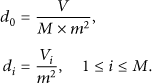
Obviously, we have

$$\begin{array}{cc}& d_{\mathrm{m}\mathrm{a}\mathrm{x}}=\max \left\{d_i\right\},\mathrm{1}\le i\le M,\end{array}$$

(2)

$$\begin{array}{cc}& d_{\mathrm{m}\mathrm{i}\mathrm{n}}=\min \left\{d_i\right\},\mathrm{1}\le i\le M,\end{array}$$

(3)

where $d_{\mathrm{m}\mathrm{a}\mathrm{x}}$ , $d_{\mathrm{m}\mathrm{i}\mathrm{n}}$ correspond to the maximum value and the minimum value of node density for all of subregions, respectively.

We introduce two metrics to classify subregions in terms of node density. The density difference ratio σ is computed by dividing the difference between the maximum node density and average node density by the difference between the minimum node density and the average node density across all subregions. The second metric, η, measures the fraction of subregions that have density higher than the average node density. Mathematically, we can define them as follows:

$$\begin{array}{cc}& \sigma =\frac{d_{\mathrm{m}\mathrm{a}\mathrm{x}}-d_{\mathrm{0}}}{\left|d_{\mathrm{m}\mathrm{i}\mathrm{n}}-d_{\mathrm{0}}\right|},\\ \eta =\frac{{\sum }_{i=\mathrm{1}}^M{\mathrm{1}}_{d_i>d_{\mathrm{0}}}}{M},\end{array}$$

(4)

where ${\mathrm{1}}_{d_i>d_{\mathrm{0}}}=\{\mathrm{0,1}\}$ is an indicator function and ${\mathrm{1}}_{d_i>d_{\mathrm{0}}}=\mathrm{1}$ implies that the node density for subregion i, $\mathrm{1}\le i\le M$ , is larger than the average value of node density; otherwise ${\mathrm{1}}_{d_i>d_{\mathrm{0}}}=\mathrm{0}$ .

To categorize subregions based on node deployment pattern, we use ${\sigma }_x$ , ${\eta }_x$ as thresholds for σ, η, respectively. According to the relationship between actual value of σ, η and their thresholds, we have the four following types of situations.

• (i)

Class I: ${\sigma }_i>{\sigma }_x$ , ${\eta }_i>{\eta }_x$ , $\mathrm{1}\le i\le M$ : this case indicates that there is a big difference between the maximum value and the minimum value of node density, and the node density is larger than the average value for the majority of subregions as well. We can tell that node density varies considerably across subregions. Therefore, Class I is deemed as target subregions with nonuniform deployment pattern.

(ii)

Class II: ${\sigma }_i<{\sigma }_x$ , ${\eta }_i<{\eta }_x$ , $\mathrm{1}\le i\le M$ : this case reveals that every subregion has similar node density, and only few regions have higher value than the average value in terms of node density. Obviously, Class II is recognized as target subregions with uniform deployment pattern.

(iii)

Class III: ${\sigma }_i>{\sigma }_x$ , ${\eta }_i<{\eta }_x$ , $\mathrm{1}\le i\le M$ : this case shows that there is a big difference between the maximum value and the minimum value of node density, and only few regions have higher value than the average value in terms of node density at the same time. Thus, this condition is not true in reality. We cannot make a decision on node deployment pattern for Class II. To solve this problem, we divide this subregion both vertically and horizontally into 4 equal subregions. Node density metrics need to recalculate for every newly generated subregion. After that, node deployment pattern is determined based on updated node density metrics.

(iv)

Class IV: ${\sigma }_i<{\sigma }_x$ , ${\eta }_i>{\eta }_x$ , $\mathrm{1}\le i\le M$ : this case demonstrates that every subregion has similar node density, and node density is larger than the average value for the majority of regions as well. We still cannot determine the node deployment pattern directly. Similar to Class III, we also partition this subregion both vertically and horizontally into 4 equal subregions. Each subregion can then be classified according the values of its node density metrics σ and η. Since both σ and η are related to the side length m of the subregion, therefore, selecting the value of m can affect values of σ and η and consequently affect the classification of the entire area. Therefore, it is necessary to select an appropriate value for m for the target area.

3.2. Multiresolution Model

We now describe the construction of the multiresolution model in detail.

3.2.1. Process of Fingerprinting

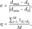
In our scenario, static sensor nodes and mobile sensor nodes coexist for different purposes. The static sensor nodes (also called anchor nodes) are deployed at the fixed locations for environment monitoring, and the mobile nodes are attached to certain monitoring objectives (e.g., collecting movement information). Every node can acquire the corresponding RSS value for every particular anchor node. Monitored results and the system performance are dependent on deployment and density of sensor nodes. Usually, RSS is utilized for localization. However, due to the existence of barriers, signal strength shows a specified amount of deviation, as shown in Figure 1. For a reference Access Point (AP) node, even with the same distances to the beacon, RSS values of two sensor nodes are not equal if one of them is related to a certain barrier. Sensor nodes residing in the same subregion are affected similarly by obstacles. Thus, RSS can be used to distinguish different subregions.

Figure 1

Comparison of received strength of signal value.

We assume n static anchor nodes are deployed in the target area. Any node not equipped with the GPS module can obtain n RSSs, denoted by $F=[f_{\mathrm{1}},f_{\mathrm{2}},\dots ,f_n]$ , where $f_i$ is the RSS value from the ith anchor node. The set of RSSs for a certain position is called a fingerprint. To deal with the instability of signal, we use the Euclidean distance as a reference to node localization. Given two fingerprints $F=[f_{\mathrm{1}},f_{\mathrm{2}},\dots ,f_n]$ and $F^{\ast }=[f_{\mathrm{1}}^{\ast },f_{\mathrm{2}}^{\ast },\dots ,f_n^{\ast }]$ , their Euclidean distance $\varphi (F,F^{\ast })$ can be computed as

$$\begin{array}{cc}& \varphi \left(F,F^{\ast }\right)=\sqrt{{\displaystyle \sum }_{i=\mathrm{1}}^n{\left(\omega \left(f_i\right)-{\omega }^{\ast }\left(f_i\right)\right)}^{\mathrm{2}}},\mathrm{1}\le i\le n,\end{array}$$

(5)

where $\omega (f_i)={\sum }_{\begin{array}{c}j=\mathrm{1},j\ne i\end{array}}^n{\mathrm{1}}_{(f_i-f_j>\mathrm{0})}(f_i-f_j)$ and ${\mathrm{1}}_{(f_i-f_j>\mathrm{0})}=\{\mathrm{0,1}\}$ is an indicator function, where ${\mathrm{1}}_{(f_i-f_j>\mathrm{0})}=\mathrm{1}$ when $f_i>f_j\hspace{0.17em}\hspace{0.17em}(\mathrm{1}\le i\le n)$ and otherwise ${\mathrm{1}}_{(f_i-f_j>\mathrm{0})}=\mathrm{0}$ .

3.2.2. Logical Region

To determine the locations of sensor nodes, we introduce a new concept, logical region, to describe whether two sensor nodes have high similarity in terms of fingerprint. $\varphi (F,F^{\ast })<\xi$ implies that these two nodes are close to each other, where ξ is a predetermined value. Intuitively, two nodes which have similar fingerprints are neighbors with high probability.

From the perspective of definition of accuracy, the larger the area a logical region covers is, the coarser the localization granularity is. Thus, a big logical region should be partitioned into a few smaller logical regions when the current granularity does not satisfy the localization requirement. In this paper, the logical region is the cornerstone of our node localization scheme. Actually, the location for a mobile sensor node is determined both by the region it belongs to and by the logical region it is situated in. Generally, the size of a logical region is related to the number of sensor nodes. A logical region with more sensor nodes covers a larger area and has a coarser granularity. On the contrary, a smaller logical region in size corresponds to a finer granularity.

3.2.3. Multiresolution Model

According to aforementioned statement, the granularity of node localization is decided by the size of a logical region. Thus, the first step is to generate logical regions. Different size of logical regions corresponds to different granularity of node localization. In other words, there is a one-to-one relationship between every size of logical regions and every granularity of node localization. Accordingly, a hierarchical localization structure is produced. In this structure, every level corresponds to a particular size of the logical region. Consequently, a multiresolution model is generated accordingly.

For the nonuniform deployment pattern, we adopt Density-Based Spatial Clustering of Applications with Noise (DBScan) [24] to clustering anchor nodes and generate logical regions. These resulting logical regions are corresponding to nodes of the tree structure. According to the granularity requirement, logical regions can be repartitioned so that smaller sizes of logical regions are generated, as shown in Figure 2.

Figure 2

Illustration of logical region for uniform deployment.

For the uniform deployment pattern, we assume that every region is a square. Every square can be divided vertically and horizontally into 4 equal subregions until the localization granularity satisfies. In this hierarchy, a region is the parent node of its subregions, and every subregion is the child node of the region. All child subregions of a particular region are situated at the same level of the tree structure, and every subregion is the sibling node of other subregions, as shown in Figure 3. Every level of the generated tree corresponds to different granularity of node localization. Furthermore, lower level regions are typically smaller and have finer localization granularity. Generally speaking, while high accuracy is preferred for most of the applications, achieving high accuracy will incur high overhead of communication and computation. Therefore, we need a tradeoff between accuracy and cost.

Figure 3

Illustration of logical region for nonuniform deployment.

We use logical region to represent all sensor nodes which reside at the lower layer and calculate the fingerprint of the logical region based on all of sensor nodes which belong to this region. In this case, the fingerprint of the logical region equals the average value of the fingerprints for all of the sensor nodes. Suppose there are k sensor nodes in this logical region, and the fingerprint for each node is $F_i=[f_{i\mathrm{1}},f_{i\mathrm{2}},\dots ,f_{in}]$ , $\mathrm{1}\le i\le k$ . Thus, we compute the fingerprint of the logical region as follows:

$$\begin{array}{l}{F}_l=\frac{F_{\mathrm{1}}+F_{\mathrm{2}}+\cdots +F_k}{k}=\{\frac{f_{\mathrm{11}}+f_{\mathrm{21}}+\cdots +f_{k\mathrm{1}}}{k},\\ \frac{f_{\mathrm{12}}+f_{\mathrm{22}}+\cdots +f_{k\mathrm{2}}}{k},\dots ,\frac{f_{\mathrm{1}n}+f_{\mathrm{2}n}+\cdots +f_{kn}}{k}\},\end{array}$$

(6)

where $F_l$ is the fingerprint for the particular logical region. As such, node localization is to determine to which logical region this node belongs, and the level of the logical region determines the granularity of node localization.

4. Multiresolution Model-Based Node Localization Scheme

4.1. System Architecture

In this subsection, the high-level architecture of NLMR is illustrated, as shown in Figure 4. The procedure of NLMR consists of three phases: fingerprinting, modeling, and localization.

Figure 4

High-level architecture of NLMR.

In the fingerprinting and modeling phase, all beacon nodes measure RSSs from other beacons. The fingerprint, which is related to RSSs of all beacons, is collected and then sent to the control center. The control center partitions the entire area into logical regions based on the fingerprint information. According to the requirement on both applications and data inquiry, a big logical region is divided again and again until the localization granularity satisfies. Corresponding levels of granularity of node localization are produced, and a hierarchical tree is generated.

In the localization phase, sensor nodes send a localization request, which includes their RSS measurement and accuracy requirement, to the control center. After comparing to the fingerprint, the control center responds with the estimated location based on the granularity of node localization.

4.2. NLMR Description

The proposed node localization scheme, NLMR, estimates the location of every sensor node in a centralized manner. NLMR aims to do its best to provide granularity of node localization as fine as possible. Figure 5 illustrates how these components interact with each other.

Figure 5

Information flow in our scheme NLMR.

4.2.1. On-Demand Localization Request by Sensor Nodes

We assume that diverse localization granularities coexist in a WSN (how to determine the localization granularity is beyond the scope of this paper). Sensor nodes send localization requests which contain both RSS measurements and localization accuracy every fixed time interval, the detailed process is as shown in Algorithm 1. We use a triple ( $A,R,T$ ) to denote the localization request message, where A represents the localization accuracy requirement, R describes RSSs received from all anchor nodes, and T stands for the timestamp at which the request is sent. There are two reasons for adding a timestamp to each node localization request. First, a timestamp can be used to identify the location of a sensor node at a specific time. Second, since our scheme deals with node localization in a centralized manner, the values of timestamps can be used to help the control center to make appropriate scheduling decisions for node localization requests.

Algorithm 1: NLMR: sensor node process.

input: localization accuracy A, RSSs from all of anchor nodes R and timestamp T.

output: location information L of a particular sensor node.

flag1: an indicator for whether the request is timeout.

flag2: an indicator for whether the request is sent successfully.

flag3: an indicator for whether the response is received successfully.

flag1 = false; flag2 = false; flag3 = false;

  (1)  for each sensor node do

  (2)   generate a request message $$(A,R,T)$$ ;

  (3)   check the lifetime of this request;

  (4)   if the request is timeout then

  (5)    flag1 = true;

  (6)    break

  (7)   end if

  (8)  end for

  (9)  for each request message do

  (10)  if flag1 = false $$\&\&$$ flag2 = false then

  (11)   send the message out;

  (12)   wait for a response message from the control center;

  (13)   while receive the response message do

  (14)    flag2 = true;

  (15)    if the response message can be parsed correctly then

  (16)     flag3 = true;

  (17)     extract location information and assign the value to L;

  (18)    end if

  (19)   end while

  (20)  end if

  (21) end for

  (22) return  L

4.2.2. Multiresolution Localization Process by the Control Center

The control center extracts the localization accuracy, RSSs measurements, and timestamp from the received request. Firstly, the control center needs to decide whether the request exceeds the time limit. The control center will neglect this request if the request times out. Secondly, the control center finds the value with coarsest granularity based on RSSs measurements and then compares to the localization accuracy. When the sensor node requires higher localization accuracy, the control center retrieves the location value with better granularity. If all the existing localization accuracies are not sufficient for the request, the control center will divide the smallest subregion into a few smaller subregions and recompute the fingerprint for the newly generated logical regions. Finally, the control center responds with the estimated location. Illustration of the multiresolution localization process is shown in Algorithm 2.

Algorithm 2: NLMR: control center process.

input: request messages with ( $$A,R,T)$$ and a multi-resolution model.

output: response messages with location information L.

flag1: an indicator for whether the request can be parsed correctly.

flag2: an indicator for whether the request is timeout.

flag1 = false; flag2 = false;

  (1)  for each request do

  (2)   parse this request;

  (3)   if the request is parsed correctly then

  (4)    flag1 = true;

  (5)   end if

  (6)   check the lifetime of the request;

  (7)   if the request is timeout then

  (8)    flag2 = true;

  (9)    break

  (10)   end if

  (11)  retrieve the location information with the coarsest granularity based R;

  (12)  while accuracy A does not be satisfied do

  (13)   if the location information is already with the highest granularity then

  (14)    divide the smallest subregion into a few smaller subregions

  (15)    recompute the fingerprint for the newly generated logical regions

  (16)    update the multi-resolution model

  (17)   end if

  (18)   require the location information with the higher granularity;

  (19)  end while

  (20)  assign the location information to L;

  (21)  send a response message including L;

  (22) end for

5. Simulation and Numerical Results

We evaluate the proposed multiresolution based localization scheme in this section. We use MATLAB to conduct the simulations. The default simulation parameters are summarized in Table 1.

Table 1

Simulation parameters.

Parameter	Value
Number of sinks	1
Number of sensor nodes	100
Number of anchor nodes	300
Simulation area	600 m ∗ 600 m
Transmission range (tr)	30 m
Value of side length m	[1, 100] m
Number of subregions M	[36, 360000]

5.1. Impact of System Parameters

The first set of simulations demonstrates the relationship between every system parameter and the side length of subregions m. We change the value of m from 1 to 100, the corresponding node density for both the maximum value and the minimum value is as shown in Figure 6, the corresponding σ is as shown in Figure 7, and the corresponding η is as shown in Figure 8.

Figure 6

Node density with respect to m.

Figure 7

σ with respect to m.

Figure 8

η with respect to m.

As we can see from Figure 6, there is an obvious difference between the maximum density and the minimum density with respect to the side length m. In Figure 6, the maximum node density jumps up to 0.0095 firstly and then decreases a little bit and fluctuates around 0.007 afterwards. At the same time, the minimum node density begins with a value close to 0 and increases gradually with m. A small m leads to tens of thousands of subregions. As a result, the number of anchor nodes is also small. Therefore, there is a big difference between the maximum node density and the minimum node density. Comparatively, a big m brings about a small quantity of subregions. There is a little difference between any two subregions in terms of the number of anchor nodes. Therefore, there is a small difference between the maximum node density and the minimum node density.

σ in Figure 7, which describes the density difference ratio, is computed by dividing the difference between the maximum node density and average node density by the difference between the minimum node density and the average node density across all regions. From Figure 7, we observe that σ obeys a normal distribution. σ reaches its maximum when the value of m is around $\mathrm{50}$ . Intuitively, this is because there is a bigger difference between the maximum node density and the minimum node density at this moment.

η in Figure 8 represents the ratio of regions for which the node density is larger than the average value of node density to the number of regions. From Figure 8, we can observe that η obeys a similar normal distribution. When the value of m is around 50, the corresponding value of η is big and stable.

5.2. Performance of Our Scheme

The second set of simulations reveals the performance and availability of our node localization scheme. Figure 9 shows the true positive percentage for judgment on node deployment with respect to the side length of subregions m. Given 100 subregions with uniform distribution and 100 subregions with nonuniform distribution, we change m from 1 to 100 and determine the pattern of node deployment for every subregion over m. From Figure 9, we recognize that the true positive ratio still obeys a similar normal distribution. More importantly, we can gain the best performance when m is around 50. The reason for this is that all system parameters have optimal value under this condition of m. There, the percentage of true positive is optimal.

Figure 9

True positive ratio for judgment on node deployment.

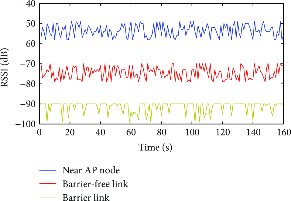
Figure 10 illustrates the true positive percentage for node localization with respect to the side length of subregions m. Given 100 sensor nodes which do not know their positions, we change m from 1 to 100 and determine the location information for every sensor node over m. From Figure 10, we recognize that the true positive ratio still obeys a similar normal distribution. More importantly, our node localization scheme verifies that NLMR can provide diverse localization granularity with high probability. Different m implies different localization accuracy which corresponds to different level of logical regions.

Figure 10

True positive ratio for node localization.

6. Conclusion

In this paper, we introduce $NLMR$ , an on-demand node localization scheme based on multiresolution model for wireless sensor networks, enabling sensor nodes to query and access the fingerprint-related location information from logical hierarchical localization structure. We show by simulations that NLMR improves the localization accuracy. We also present the fact that our node localization scheme can provide location information with diverse localization granularities.