Collaborative Routing Protocol Based on Hydrodynamics for Wireless Sensor Networks

Abstract

Collaborative routing protocol design is hard work for wireless sensor networks (WSNs), especially for the large scale WSNs. The complexity and collaboration associated with the routing protocol design must be taken into account. A collaborative hydrodynamics routing (HR) protocol based on hydrodynamic theory is proposed in this paper, which aims at prolonging the network lifetime and adapting to the variety of network scales. Packets for forwarding in sensor networks can be analogous to fluid elements moving in a fluid field. Sink nodes are similar to the sink flows and source nodes are similar to the source flows; and packets would flow from sources to sinks under potential flow. Simulation results show that our approach has a great advantage as it offers a significant improvement in the aspects of decreasing complexity and prolonging network lifetime and demonstrates high performance for the improvement in collaboration of routing protocol. Comparing with conventional AODV protocol, HR achieves higher successful delivery rate and longer network lifetime by 50% and 40%, respectively.

1. Introduction

In recent years, with the advancement of sensor technology, as well as the development of low-energy electronic and RF (radio frequency) technology, low-energy and low-cost wireless sensors had been widely applied in practices [1–4]. Routing protocol played a key role in high performance wireless sensor networks. However, the design of routing protocol was always hard work, especially for the large scale wireless sensor networks. Some researchers mapped the problems in sensor networks to classical physical problems, such as electrostatics, optics, percolation theory, and diffusion [5]. In this paper, we mapped the routing problem to hydrodynamic problem.

Toumpis and Tassiulas [6] firstly introduced the electrostatic field theory into wireless sensor networks, when researching node deployment of large scale wireless sensor networks. Then, they did further work in [7, 8]; although focusing on the deployment of sensor nodes in wireless sensor networks, this approach actually abstracted the optimal deployment of nodes into charge distribution of electrostatic field, which provided an effective ideology for us to build the routing model. When solving the routing problem of ad hoc networks, Kalantari and Shayman [9, 10] analogized sensor networks as electrostatic fields. On this basis, a series of partial differential equations was deduced according to the nature of electrostatic field, and nodes’ routing was figured out by solving these partial differential equations. In [11, 12], the authors further extended the methods in [9, 10] to the situations with multiple sinks and various loads; by analogizing multisink sensor network as electrostatic field, the optimal routing and load distribution algorithm for multisink sensor networks was proposed. Ghica et al. [13] investigate the security aspects of electrostatic field-based routing (EFR) protocols. They focus on an instance of EFR, called multipole field persistent routing (MP-FPR), for which they identify attacks that can target different components of the protocol and propose a set of corresponding defense mechanisms.

When studying the routing of sensor networks, Huang et al. [14] put forward a magnetic diffusion (MD) algorithm based on magnetic field. The algorithm abstracted sinks into magnets, and data into scrap iron that could be attracted by magnets, so as to establish a magnetic field triggered by magnet. Data is routed to sinks according to nodes’ magnetic intensity in the field. MD algorithm realizes real-time and reliable transmission of data, enabling the efficient use of energy by nodes in the network. However, for ordinary sensor networks, MD algorithm is unable to evenly make use of network resources. In [15], the authors propose an efficient data dissemination algorithm called coordinate magnetic (CM) for mobile sinks wireless sensor networks. This algorithm is based upon representing the network as a virtual grid and using coordinate conception and magnetic phenomenon for data dissemination in network.

Catanuto et al. [16, 17] put forward a sensor network routing algorithm based on geometrical optics. This algorithm abstracted data transmission in networks as light transmission with certain refractive index, so as to figure out the routing of the network. Baumann et al. [18, 19] abstracted the network as a thermal field triggered by a heat source. As for this, data will route according to nodes’ temperature in the network, so as to reach the heat source (sink). Ghica et al. [20] introduced a methodology based on Bezier curves as guiding trajectories in the routing process, where the relay nodes could determine locally the Bezier curve they belonged to which required only the transmission of the so-called control points that determine the shape of one (boundary) curve.

In the above related works, researchers have made great contributions to the analysis and design of sensor network routing. However, they seldom solve the routing problem from the view of hydromechanics. As for this, in our work, sensor network routing will be explored with theories in hydromechanics since they have plenty of similarities. In potential flow theory, there exist two kinds of points: point source and point sink. Point source diverges fluid, which is similar to source nodes’ sending out data in sensor networks. While, point sink converges fluid, which is similar to sink nodes’ receiving data in sensor networks. Fluid from point source finally converges in point sink; this process is exactly similar to that in which source nodes send data to sink nodes in sensor network.

The main contribution of this paper has three points. First of all, we will be able to solve the routing problem of sensor networks through hydrodynamics theory. What is more is that, shown by theoretical analysis and experimental simulation, the routing algorithm based on hydrodynamics proposed in this paper is able to realize real-time and reliable transmission of data, as well as to improve the collaboration of nodes. Finally, compared with other routing schemes, our algorithm shows less latency, higher throughput, lower energy consumption, and better energy efficiency.

The rest of this paper is organized as follows. Section 2 introduces related work on fluid field routing. Section 3 introduces basic knowledge called potential flow. Section 4 establishes routing model and proposes our routing algorithm. Section 5 makes use of simulation tools to simulate the routing protocol. Finally, Section 6 concludes the paper and discusses some future work.

2. Related Work

In the last several years, some researchers had discussed the hydrodynamic method used in wireless sensor networks. Pac et al. [21] presented a novel hydrodynamic simulation method to solve the deployment problem of mobile sensor networks in an unknown environment. This method is based on the physical law in hydrodynamics theory, modeling sensor network as inviscid and compressible fluid, and regarding each node in the network as fluid element. As for this, the diffusivity of fluid drove nodes to “flow” with fluid, so as to make the network deployment with an expected effective coverage rate. Although [21] dealt with the node deployment work of sensor networks, its ideology provided us with valuable inspiration for subsequent researches. Different from [21], we modeled the whole sensor network as a fluid field and considered packet transmission a flowing of fluid, while [18] only regarded nodes as fluid elements.

Gribaudo et al. [22] presented a wireless sensor network analysis model based on hydrodynamics. In the model, sensor nodes were taken as fluid entity and distributed in a smooth and continuous space. The authors had defined the concept of local node density, which referred to the quantity of nodes distributed in unit area of the given space. They assumed that nodes in networks were static. Nodes transmitted information received to other nodes by multihop. This mode confined network in a simplified state. Yet, it still solved many problems, such as nodes’ energy consumption and nodes’ contending for wireless channels, as well as communication routing.

This paper absorbed the research findings in [22]. Applying hydrodynamics in network model can help to reduce the complexity of calculation when dealing with large scale sensor networks. Owning to the large quantity and the uneven distribution of nodes, large scale sensor networks may lead to overcomplexity or failure of normal routing strategy. Network model based on hydrodynamics can bypass the network scale problem; that is, the network model was smooth no matter what the size of network was. So as to avoid the influence of network scale, at the same time, simplify the routing strategy.

Khawam et al. [23] proposed a fluid model to analyze ad hoc wireless networks. This fluid model represented infinite nodes with equivalent continuums and described the property of continuums with node density. In this model, nodes were distributed in the network according to certain distribution function. The key to this model was to utilize a simple and direct method to fully consider jamming effect, CSMA/CA mechanism, and wireless transmission effect. The literature provided a closed formula for node average energy and range probability. Moreover, it had estimated node density variation, network scale, and carrier sensing range of the whole network. Chiasserini et al. [24] put forward a fluid model designed for large scale wireless sensor network. It was nonsense to describe networks with large volumes of sensor nodes via some microcosmic properties, such as node position and communication rate. Fluid model presented by the literature put to use some simple hypotheses, which made the problem easier to be solved. However, this mode still solved plenty of difficulties, such as energy consumption, nodes’ active and sleeping mode, channel contending, confliction of parallel transmission, and communication routing. Kim and Jennifer [25] demonstrated the advantage of fluid mode from another dimensionality. The literature established a simulation based on fluid model, which helped to reduce the calculation volume of large scale network simulation. In simulation based on fluid mode, a cluster of spatially dense data packet simulated a fluid micelle at specified time point. Behavior of this fluid micelle in continuous or discrete time domain was described with a series of mathematical formula. Large quantities of data packet were abstracted into a fluid micelle, so as to reduce the calculation load.

Although to apply hydrodynamics in network model is no longer novel, it is still quite rare to establish routing model with hydrodynamic theories, as well as to study the routing strategy from this viewpoint. In this paper, the routing problem, based on previous researches, will be further explored.

3. Preliminaries: Potential Flow

Potential flow is frictionless, irrotational flow. Even though all real fluids are viscous to some degree, if the effects of viscosity are sufficiently small then the accompanying frictional effects may be negligible.

3.1. The Velocity Potential

In potential flow, we can define a potential function, Φ, as a continuous function that satisfies the basic laws of fluid mechanics: conservation of mass and momentum, assuming incompressible, inviscid, and irrotational flow. The velocity field V is irrotational. This means that

$$\begin{array}{cc}& \nabla \times \mathbf{V}=\mathrm{0}.\end{array}$$

(1)

When $\nabla \times \mathbf{V}=0$ the rate of rotation of an infinitesimal element of fluid is zero. From vector calculus, we know that if a velocity field is irrotational then it can be expressed as the gradient of a “scalar potential” Φ:

$$\begin{array}{cc}& \mathbf{V}=\nabla \Phi .\end{array}$$

(2)

In 2, $\Phi =\Phi (x,y,z,t)$ is the “velocity potential,” using the definition of the ∇ operator. As such the components of velocity in Cartesian coordinates, as functions of space and time, are

$$\begin{array}{cc}& u=\frac{\partial \Phi }{\partial x},\hspace{1em}\hspace{1em}v=\frac{\partial \Phi }{\partial y},\hspace{1em}\hspace{1em}\mathrm{\hspace{0.17em}\hspace{0.17em}}w=\frac{\partial \Phi }{\partial z}.\end{array}$$

(3)

If, in addition, the flow is incompressible, then

$$\begin{array}{cc}& {\nabla }^{\mathrm{2}}\Phi =\mathrm{0}.\end{array}$$

(4)

3.2. Potential Lines and Streamlines

Lines of constant Φ are called potential lines of the flow. In two dimensions

$$\begin{array}{cc}& d\Phi =\frac{\partial \Phi }{\partial x}dx+\frac{\partial \Phi }{\partial y}dy\\ d\Phi =udx+vdy.\end{array}$$

(5)

Since $d\Phi =0$ along a potential line, we have

$$\begin{array}{cc}& \frac{dy}{dx}=-\frac{u}{v}.\end{array}$$

(6)

Recall that streamlines are lines everywhere tangent to the velocity, so potential lines are perpendicular to the streamlines. This is because inviscid and irrotational flow is indeed quite pleasant to use potential function, Φ, to represent the velocity field, as it reduced the problem from having three unknowns $(u,v,w)$ to only one unknown (Φ). Streamline function is represented by Ψ. Lines of constant Ψ are perpendicular to lines of constant Φ, except at a stagnation point.

Luckily Φ and Ψ are related mathematically through the velocity components:

$$\begin{array}{cc}& u=\frac{\partial \Phi }{\partial x}=\frac{\partial \Psi }{\partial y}\\ v=\frac{\partial \Phi }{\partial y}=-\frac{\partial \Psi }{\partial x}.\end{array}$$

(7)

Equations 7 are known as the Cauchy-Riemann equations which appear in complex variable math.

3.3. The Principle of Superposition

Equation 4 shows that, for a two-dimensional, irrotational, incompressible flow, the velocity potential obeys “Laplace's equation” and so does the stream function. That is

$$\begin{array}{cc}& {\nabla }^{\mathrm{2}}\Phi =\mathrm{0},\hspace{1em}\hspace{1em}{\nabla }^{\mathrm{2}}\Psi =\mathrm{0}.\end{array}$$

(8)

Since Φ and ψ obey the same differential equation (for 2D, irrotational, incompressible flow), a solution to one potential flow problem can be directly used to generate a solution to a second potential flow by interchanging Φ and ψ. Specifically, if ${\Phi }_1$ and ${\psi }_1$ represent potential flow 1, then the interchanges ${\Phi }_2={\psi }_1$ and ${\psi }_2=-{\Phi }_1$ will represent some other potential flow 2. The minus sign in ${\psi }_2=-{\Phi }_1$ is needed to ensure consistency in the sign of the velocity components derived from Φ and ψ.

Different potential flows can be added together to generate new potential flows (the Principle of Superposition). Laplace's equation (equation 8) is linear. The linear property means that if the stream function and velocity potential are known for two different flows, say flows 1 and 2, then the sum of flows 1 and 2 will also be a solution to Laplace's equation. By “solution to Laplace's equation” we mean that, if ${\nabla }^2{\psi }_1=0$ and ${\nabla }^2{\psi }_2=0$ , then

$$\begin{array}{cc}& {\nabla }^{\mathrm{2}}({\Psi }_{\mathrm{1}}+{\Psi }_{\mathrm{2}})={\nabla }^{\mathrm{2}}{\Psi }_{\mathrm{1}}+{\nabla }^{\mathrm{2}}{\Psi }_{\mathrm{2}}=\mathrm{0}.\end{array}$$

(9)

Here, ${\psi }_1$ is the stream function for flow 1 and ${\psi }_2$ is the stream function for flow 2. Equation 9 shows that the sum of the stream functions for flows 1 and 2 is also a solution to Laplace's equation. Same comments apply to the sum of the velocity potentials, ${\Phi }_1+{\Phi }_2$ , for flows 1 and 2.

3.4. Source and Sink Flows

Consider the z-axis (into the page) as a porous hose with fluid radiating outwards or being drawn in through the pores. Fluid is flowing at a rate Q (positive or outwards for a source, negative or inwards for a sink) for the entire length of hose, b. For simplicity take a unit length into the page ( $b=1$ ) essentially considering this a 2D flow (Figure 1).

Figure 1

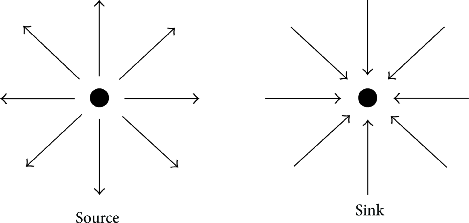
Source ( $Q>0$ ) and sink ( $Q<0$ ).

The source is located at the origin of the coordinate system. From the figure above you can see that there is no circumferential velocity, but only radial velocity. Thus the velocity vector is

$$\begin{array}{cc}& \begin{array}{c}{v}_r=\frac{Q}{\mathrm{2}\pi r}\\ v_{\theta }=\mathrm{0}\end{array}⟹\left\{\begin{array}{cc}{v}_x=\frac{Q}{\mathrm{2}\pi }\frac{x}{x^{\mathrm{2}}+y^{\mathrm{2}}}\hfill & \hfill \\ v_y=\frac{Q}{\mathrm{2}\pi }\frac{y}{x^{\mathrm{2}}+y^{\mathrm{2}}}.\hfill & \hfill \end{array}\right.\end{array}$$

(10)

In 10, the left part denotes the flow in cylindrical coordinates while the right part represents the flow in Cartesian coordinates. Q is the total volumetric flow rate outward from the source, per unit depth into the page. $Q>0$ for a source; $Q<0$ for a sink. Equation 10 for $v_r$ ensures that the total radial volumetric flow rate is constant. In other words, at each radial distance from the source or sink, the volumetric flow rate per unit depth, given by $2\pi r\hspace{0.17em}\hspace{0.17em}{v}_r$ , equals the constant Q.

Integrating the velocity we can solve for Φ and ψ:

$$\begin{array}{cc}& \Phi =\frac{Q}{\mathrm{4}\pi }\ln \left(x^{\mathrm{2}}+y^{\mathrm{2}}\right),\hspace{1em}\hspace{1em}\Psi =\frac{Q}{\mathrm{2}\pi }\text{arctg}\frac{y}{x}.\end{array}$$

(11)

4. Routing Mechanism Based on Potential Flow

Routings, as we know, are the paths which begin from the source nodes and end with the sink nodes. Source nodes produce messages continuously and send them to the sink nodes and, at the same time, sink nodes receive them. So, the source nodes and sink nodes in wireless sensor networks can be analogousto source points and sink points in hydrodynamics.

4.1. Analogy with Hydrodynamics

The first typical macroscopic quantity, employed in many of the others’ works [5, 8], is the node density function $d(\mathit{r})$ , measured in nodes per m² and defined by the limit 12, in which a set A of incremental size $\left|A\right|$ contains the point $\mathit{r}=(x,y)$ and covering $N(A)$ nodes:

$$\begin{array}{cc}& d\left(\mathbf{r}\right)=\underset{\left|A\right|\to \mathrm{0}}{\lim }\frac{N\left(A\right)}{\left|A\right|}.\end{array}$$

(12)

Therefore, the total number of nodes in the whole network is given by the two-dimensional integral $N=\int d(x,y)dS$ .

The next macroscopic quantity described here is the information density function $\rho (x,y)$ , which is measured in bps/m² and jointly describes the distributed sets of sources and sinks. In a location $(x,y)$ where $\rho (x,y)>0$ , there is a distributed set of sources, which jointly create traffic with rate $\rho (x,y)\epsilon$ over any set of incremental areas ε centered at $(x,y)$ . Similarly, as we described earlier, the source flow in potential flow has the same behavior where $Q>0$ .

The last macroscopic quantity used in many papers is the traffic flow function $\mathbf{T}(x,y)=T_x(x,y)\widehat{\mathbf{x}}+T_y(x,y)\widehat{\mathbf{y}}$ , which is a vector function measured in bps/m and models the flow of traffic at location $(x,y)$ . Its direction gives the direction of the traffic flow, and its magnitude gives the intensity of the traffic. We note that the traffic flow function $T(x,y)$ describes the way the traffic moves across the network and the information density function $\rho (x,y)$ describes how the traffic is created or absorbed. Clearly, they both have close relation to the potential flows, the traffic flow function $T(x,y)$ is analogous to velocity field V, and the information density function $\rho (x,y)$ is analogous to fluid flow rate Q.

4.2. Collaborative Routing Model

We will begin with a simple single-source and single-sink model. Complicated networks (such as multisource and multisink) may be processed with the superposition theorem mentioned previously, that is, superposition of multiple single-source and single-sink models. As is shown in Figure 2, the source node ( $Q>0$ ) is located at the upper left corner, while sink node ( $Q<0$ ) is located at the lower right corner. The plot on the left shows velocity vectors and potential lines, while the right plot presents potential lines and streamlines. There are several streamlines from source to sink, while these streamlines are orthogonal to potential lines. If a sensor network has large volumes of nodes (dense nodes), by connecting nodes nearby the stream lines along the direction, we may get several paths. These paths provide multiple links (i.e., route) from the source node to sink node. It is true that the number of practical paths would not be as much as the number shown in the figure, for the number of nodes is limited.

Figure 2

Single-source single-sink model: velocity vectors and potential lines (a), potential lines and streamlines (b).

Taking into consideration the complexity of practical sensor networks, we promote the aforementioned single-source and single-sink model to multisource and multisink model. According to the superposition theorem discussed in Section 3.3, when sensor networks have multiple source nodes and sinks nodes, the nodes will be regarded as sources and sinks in hydrodynamics. Fluid fields created by these sources and sinks may be superposed together. As shown in Figure 3, sink node 1 ( $Q<0$ ) is located at the upper left corner and sink node 2 ( $Q<0$ ) is located at the lower right corner, while the four source nodes are dispersed in the network. It can be seen from the figure that there are streamlines between source node 3 (between the two sink nodes) and sink node 1, as well as between source node 3 and sink node 2. In other words, source node may “flow” to 2 sink nodes at the same time. Being “blocked” by source node 2, source node 1 could only “flow” to sink node 1. These features comply with hydrodynamic theories. As a matter of fact, the model we established is just based on the theory of hydrodynamics.

Figure 3

Multisource Multisink model: velocity vectors and potential lines (a), potential lines and streamlines (b).

4.3. Collaborative Routing Algorithm

After the deployment of nodes, the next step is to establish route according to the routing algorithm. Assuming that sinks and sources are able to acquire their coordinate information (e.g., GPS, RSSI) with some location methods, sources are to produce a broadcast packet (Msg_broadcast), which contains packet type, coordinates, load value (the value of Q), hop count, and other fields, and then broadcast the packet out. Intermediate nodes will forward the packet after receiving it, and finally the packet will arrive at sinks. Normally, we will set up a maximum coverage radius (R_sink) for sinks. It is true that such radius may also be replaced by allowable maximum hop count, so as to segment the area. This is similar to clustering operation. Sinks will create the member list of sources (List_src) according to the coordinates or hop count information contained in the broadcast packet. After having obtained the list, coordinates, load, and other related information, sinks will compute according to these information so as to get the superposed Φ and ψ. Then, sinks will produce a routing request packet (Msg_request), which contains packet type, hop count, Φ and ψ, and velocity vector of current node. The request packet will then be broadcasted in their coverage scope. When neighboring nodes receive the request packet, they will extract Φ and ψ and figure out their own velocity vectors by simple calculation. Then they choose nodes having smallest included angle as their previous hop nodes and send out routing confirmation packet (Msg_ack) to these previous hop nodes. The confirmation packet contains information of packet type and the previous hop node's ID. Procedure of the algorithm is shown in Figure 4.

Figure 4

Establishment of route.

In order to better describe the process, please refer to Figure 4. Intermediate node C receives request packet from neighboring nodes A and B at the same time. Node C calculates the velocity vector included angle with A and B, separately denoted as $\theta a$ and $\theta b$ . Then, the value of $\theta a$ and $\theta b$ will be compared ( $\theta a<\theta b$ ). So node C will select node A as its previous hop node since node A has smaller included angle. Then, node C will send routing confirmation packet to node A and establish routing list to record A as its previous node. After node A receives the routing confirmation packet sent by node C, it will update the routing list and take C as the next hop node. The process goes in this way until the sources send out routing confirmation packet to sinks, and a complete routing path between sinks and sources will be successfully established.

The whole routing algorithm may be demonstrated with Algorithm 1.

Algorithm  1. Routing Algorithm of Hydrodynamics.

• (1)

Source Node produces and sends out broadcast packet (Msg_broadcast);

(2)

Intermediate Node receives and forwards the broadcast packet;

(3)

Sink Node receives the broadcast packet, and figures out the included source node list (List_src);

(4)

Sink Node calculates according to the member list and obtains the superposed Φ and ψ;

(5)

Sink Node produces routing request packet (Msg_request) and sends out the packet within the coverage radius (R_sink);

(6)

Intermediate node (i) receives the routing request packet and extracts Φ and ψ;

(7)

Intermediate node (i) calculates it own velocity vector and chooses the minimum included angle min $\{\theta i\}$

(8)

Intermediate node (i) sends out routing confirmation packet (Msg_ack) to its previous node ( $i-1$ );

(9)

Intermediate node (i) constructs routing list, recording node ( $i-1$ ) as node of previous hop;

(10)

Intermediate node ( $i-1$ ) receives routing confirmation packet (Msg_ack);

(11)

Intermediate node ( $i-1$ ) updates the routing list, recording node (i) as node of the next hop;

(12)

Intermediate node (i) constructs and sends out the new routing request packet;

(13)

The rest can be done in the same manner, until the routing request packet arrives at the source;

(14)

Source Node sends out routing confirmation packet to sink node;

(15)

With the method, multiple routing paths between sinks and sources are established.

We construct a plane region A with the area of $1000*1000$ and randomly distribute 300 sensors and 1000 sensors, respectively. The sink is located at the center of region A, while the four sources are separately located at the four corners (as is shown in the left plot of Figures 5 and 6). According to the routing algorithm shown in Figures 5 and 6, we established the routing path for nodes in region A, as is shown in the right plot of Figures 5 and 6.

Figure 5

Demonstration of hydrodynamics routing algorithm with 300 sensors.

Figure 6

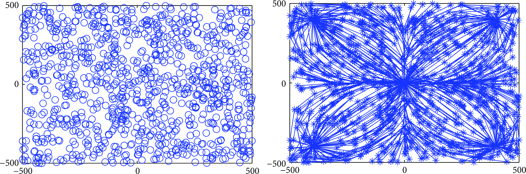
Demonstration of hydrodynamics routing algorithm with 1000 sensors.

Comparing Figure 5 with Figure 6, we can see that the smoothness of path is determined by node density. Higher density leads to better smoothness. No matter what the sensor number is, the network has similar routing paths, since we take the whole network as a fluid field, regardless the scale of the network.

4.4. Routing Maintenance

Sensor networks are often deployed in the complicated environment. As a result, nodes often fail because of various reasons, such as lower power and damage. Failed nodes may lead to failure of packet transmission. Thus, it is necessary to maintain and update the route. Sources may periodically send maintenance packet to sinks. If there exist failed nodes on the paths, routing maintenance or update is hereby required. When new nodes are added, sinks may not establish a new route immediately owning to overhigh cost. Instead, sinks will preserve newly added nodes as backup. When failed nodes come up, new nodes will be used to replace the failure ones. In this way, expenses on route establishment are saved and the network lifetime is extended.

5. Simulation Results and Analysis

Because a variety of routing algorithms for wireless sensor network have been developed and each algorithm has its own scenario, it is hard to compare all these algorithms. The solution is given by Rmase [26] which deals with the challenge to compare different routing algorithms. Rmase application, written in Matlab code, is the base application we used to run all our simulations. Rmase consists of a network topology model, an application model, and a performance model. Rmase has been used to develop new routing algorithms, to analyze performance tradeoffs. Rmase is implemented as application in Prowler [27]. The simulation was done in Prowler, which is an event based simulator, a framework based on TinyOS/NesC. Rmase provides a set of performance metrics for comparing different routing algorithms, including latency, throughput, success/loss rate, and energy consumption/efficiency.

• (1)

Latency: the time delay of an event sent from the source node to the destination node. We reported it in seconds (s). Network latency is then averaged by the number of destinations as shown in Figure 7.

(2)

Throughput: number of messages per second received at destination. The throughput of the network is the sum of the throughputs from all destinations. The throughput of the network is the sum of the throughputs from all destinations as shown in Figure 8.

(3)

Success rate: the total number of packets received at all the destinations versus the total number of packets sent from all the sources. It measures the overall success of the network. We reported it in percentage (%).

(4)

Energy consumption: the total energy consumed by the nodes in the network during the period of the experiment (Joules).

Figure 7

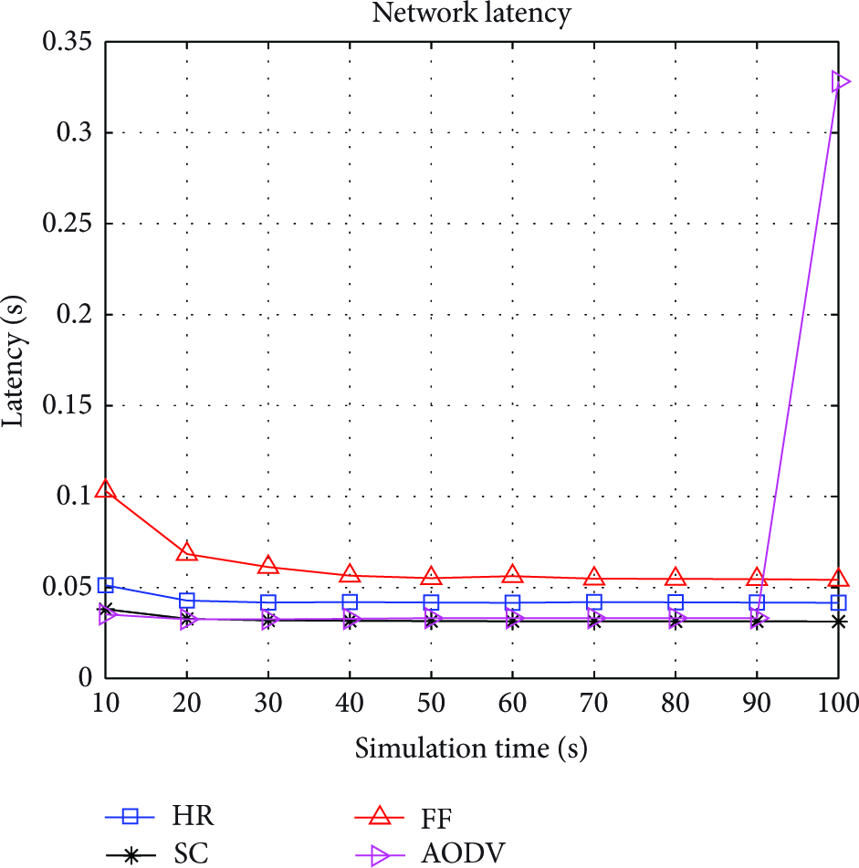
Network latency.

Figure 8

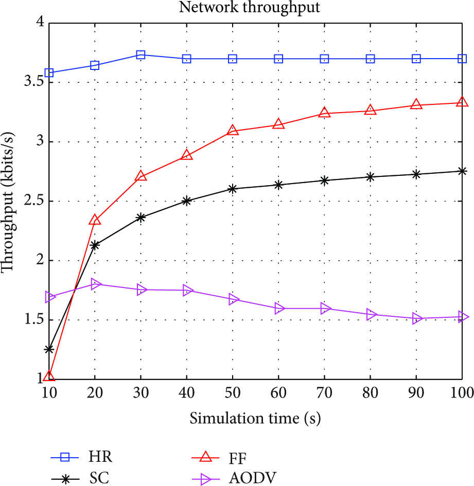
Network throughput.

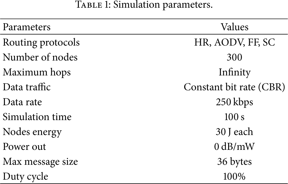
We choose three classical multipath routing protocols to compare with Ad hoc on-demand distance vector (AODV) routing protocol, flooded forward ant routing (FF) [28], and sensor driven and cost-aware ant routing (SC) [28]. Zhang et al. in SC assume that ants have sensors so that they can smell where there is food at the beginning of the routing process so as to increase in sensing the best direction that the ant will go to initially. FF argues the fact that ants even augmented with sensors can be misguided due to the obstacles or moving destinations.

Table 1 provides the simulation parameters.

Table 1

Simulation parameters.

Parameters	Values
Routing protocols	HR, AODV, FF, SC
Number of nodes	300
Maximum hops	Infinity
Data traffic	Constant bit rate (CBR)
Data rate	250 kbps
Simulation time	100 s
Nodes energy	30 J each
Power out	0 dB/mW
Max message size	36 bytes
Duty cycle	100%

In Figure 7, latency in HR (hydrodynamics routing) case is much less than latency in FF while being a little higher than SC and AODV. For HR contains a few paths from the source node to sink node, including the shortest path, the average hops of all the paths are longer than that of the shortest path, so it takes a little more time to deliver the packets to the sink. We have calculated the average network latency throughout the simulation for the HR case which is 0.0453 sec and 0.036 for the AODV. In HR latency is increased by approximately 25%.

In Figure 8, we observe that throughput in HR is higher than that in the other three, because HR can send packets on different paths simultaneously while AODV, for example, has only one path (implying that we consider 100% delivery rate). In HR case the total packets sent to the destination are much more than the packets sent by sources in the AODV case (about 1352 packets sent in HR and 406 packets in AODV case, which is about 30% of the HR packets.). Also we see that in SC and FF cases the graph of throughput tends to be increasing. This does not happen in HR case in which the graph is not increasing but tends to converge around 3.75. In HR case for the whole simulation time throughput is higher than 3.5 and maximum measured value is above 3 messages per second. Consequently, since throughput measures the received packets at destination per second, the throughput figure is analogous to success rate.

We can see from Figure 9 that in HR case success rate for a long portion of simulation time is higher than 90%. This means that more packets are likely to be delivered to the destination. Approximately after 30 seconds in HR case the success rate is near 92%. On the contrary, in other three cases, we observe that the success rate is rather low at the beginning of the simulation. Also we can see that in SC and FF cases the success rate is increasing while in AODV case it is decreasing. The maximum difference in success rate measurements in all cases reaches about 50%.

Figure 9

Network success rate.

As we can see in Figure 10, the network energy consumption is keeping increasing in all cases. The AODV case has the highest energy consumption and SC case has the lowest one. Also we can see that the difference in energy consumption (energy_AODV(i) − energy_HR(i) for $i=1\cdots 100$ ) is greater than zero and keeps increasing. That shows us that if we continue simulation for more than 100 seconds energy consumption in HR keeps decreasing compared to AODV. That observation is very important in a sensor network.

Figure 10

Network energy consumption.

6. Conclusions and Future Work

The paper puts forward a sensor network collaborative routing model based on hydrodynamic theory. In this model, there is no need to consider the scale of the whole network. The whole network is abstracted as a fluid field. Sources and sinks in the fluid field separately disperse and absorb fluid, which is similar to source nodes’ sending out packet and sink nodes’ receiving packet in sensor networks. Streamlines formed between sinks and sources in fluid field provide reference for use to establish the routing strategy. By tracking the route along the streamlines between nodes, we will be able to establish multiple paths from sources to sinks. In the research, single-source single-sink mode and multisource single-sink model are proposed. Collaborative routing algorithm is established according to the model. Eventually, the performance of the routing algorithm is evaluated on Prowler and Rmase simulation platform. The simulation parameters have chosen network latency, throughout, energy consumption, and energy efficiency. Shown by the simulation result, the algorithm has good performance.

This paper only conducts preliminary research on routing algorithm of hydrodynamics. Many problems still need to be further studied, such as the adaptability of the routing algorithm to network scale and to network topology variation.