A DCT Regularized Matrix Completion Algorithm for Energy Efficient Data Gathering in Wireless Sensor Networks

Abstract

This paper presents a novel matrix completion algorithm to enable energy efficient data gathering in wireless sensor networks. The algorithm takes full advantage of both the low-rankness and the DCT compactness features in the sensory data to improve the recovery accuracy. The time complexity of the algorithm is analyzed, which indicates it has a low computational cost. Moreover, the recovery error is carefully analyzed and a theoretical upper bound is derived. The error bound is then validated by experimental results. Extensive experiments are conducted on three datasets collected from two testbeds. Experimental results show that the proposed algorithm outperforms state-of-the-art methods for low sampling rate and achieves a good recovery accuracy even if the sampling rate is very low.

1. Introduction

Wireless sensor networks (WSNs) have been widely used in a variety of applications such as precision agriculture [1], personal health monitoring [2], and environment surveillance [3], in which sensor nodes with limited battery energy are deployed and periodically report their sensor readings to the base station or sink node. Therefore, a key issue in wireless sensor networks is how to efficiently gather these data from sensors provided with only limited energy resources. In the classical data gathering approach [4], each sensor node simply forwards its sensor readings to the sink, resulting in a large amount of traffic and energy consumption.

Recently, Compressive Sensing (CS) [5, 6] has emerged as a new approach to tackle the efficient data gathering problem in WSNs. Taking advantage of the sparsity in sensor readings, CS based methods [7–9] require fewer data packets than the classical approach. However, there are many practical problems when applying CS to data gathering in WSNs. Firstly, CS based methods require a prior dictionary to sparsify the sensor readings. Secondly, the measurement matrix in CS is composed of independent and identically distributed random Gaussian entries, which is dense with very few zero elements. Therefore, sensor nodes need to sample all sensor readings and perform a considerable number of measurement operations, resulting in a large amount of energy waste. Thirdly, CS requires the number of measurements to exceed a certain threshold (depending on the sparsity level of sensor readings) to achieve exact recovery. However, the realistic sensor signal is not always exactly sparse as it should be. Therefore, low sampling rate may lead to insufficient measurements and result in a bad recovery accuracy.

As an extension of CS, matrix completion [10] has shown its potential for enabling efficient data gathering in WSNs. Because the sensor readings are highly temporal-spatial correlated, the data matrix structured by the sensor readings will approximate to a low-rank matrix. Therefore, the sink node can gather only a few of the total sensor readings and adopt the matrix completion algorithm to reconstruct the missing data. However, unlike CS based methods, matrix completion based methods do not require the prior dictionary to sparsify the original signal. Furthermore, the sampling matrix (or measurement matrix) in matrix completion is much sparser than CS, which makes it more suitable for wireless sensor networks.

Utilizing the low-rankness feature in sensory data, there are many pioneering works [11–13] on applying matrix completion to WSN, which adopt the alternating least squares technique to estimate the low-rank matrix. The recovery accuracy is further improved by utilizing the spatiotemporal structure in the WSN data. However, the improvement is limited because the spatiotemporal structure directly implies the low-rank feature, and in some sense, these two features are equivalent. Moreover, the alternating least squares algorithm does not scale to large rank.

Besides the low-rankness feature, we observe that the sensor readings in WSNs also exhibit Discrete Cosine Transform (DCT) compactness feature. In other words, the sensor readings can be approximated by only a small number of DCT coefficients. Therefore, by taking full advantage of the DCT compactness feature of the WSNs data, in this paper, we propose a DCT Regularized Matrix Completion (DRMC) algorithm. We analyze the time complexity of DRMC, which indicates that the proposed algorithm has a low computational cost. Moreover, we analyze the recovery error of DRMC and derive a theoretical upper bound. The error bound is then validated by experimental results. Extensive experiments are carried out on three datasets that are collected from two realistic WSN testbeds. We compare the performance of DRMC with state-of-the-art methods. Experimental results show that DRMC outperforms state-of-the-art methods for low sampling rate and achieves a good recovery accuracy even if the sampling rate is very low.

The main contributions of this paper are summarized in the following:

• (i)

We examine the sensor data collected from real-world WSNs, which reveal two data features: (1) low-rankness, (2) DCT compactness.

(ii)

Inspired by these observations, we design a novel DCT Regularized Matrix Completion (DRMC) algorithm to estimate the missing sensory data. Experimental results indicate that DRMC outperforms state-of-the-art methods when the sampling rate is low.

(iii)

We analyze the time complexity of the DRMC algorithm, which indicates that DRMC has a low computational cost.

(iv)

We analyze the recovery error of the DRMC algorithm and derive a theoretical upper bound, which is then validated by experimental results.

The rest of this paper is organized as follows. Section 2 reviews the state-of-the-art methods. Section 3 models the problem. Section 4 examines the data features in WSNs. Section 5 proposes the DRMC algorithm. Section 6 analyzes the time complexity of the algorithm. Section 7 analyzes the recovery error of the algorithm. Section 8 evaluates the effectiveness of the proposed algorithm. Section 9 concludes this paper.

2. Related Works

In this section, we make a brief review of previous works related to the data gathering problem in wireless sensor networks.

2.1. Compressive Sensing

Compressive Sensing (CS) theory suggests that sparse signals can be accurately reconstructed from only a small number of measurements [5, 6]. It is a new paradigm for signal processing of networked data [7] and there are many CS based methods for data gathering in wireless sensor networks. Luo et al. proposed a data gathering scheme that applies Compressive Sensing theory to reduce communication cost [14]. Quer et al. presented a framework for data gathering and signals recovery in actual WSN deployments with the integration of CS [9]. Ebrahimi and Assi recently proposed a decentralized method to apply the Compressive Sensing to data gathering in wireless sensor networks [15].

2.2. Matrix Completion

Recently, there are many applications that apply matrix completion technique to wireless sensor networks. Utilizing the low-rankness and spatiotemporal correlation, Zhang et al. proposed a method to recover the lost data in internet traffic matrices [13]. Kong et al. designed an algorithm using the low-rank structure, time stability, space similarity, and multiattribute correlation to estimate the missing data in highly incomplete data matrix [12]. Cheng et al. presented a Spatiotemporal Compressive Data Collection (STCDG) algorithm that utilizes the low-rankness and short-term stability features to reduce data traffic in WSNs [11].

In our earlier work [16], we have studied the data recovery problem in wireless sensor networks when historical data are available and proposed a DCT-Regularized Partial Matrix Completion (DCT-RPMC) algorithm. However, the new algorithm proposed in this paper does not depend on any historical data, which greatly widens its applicability to more general scenarios.

3. Problem Formulation

In this section, we formally formulate the data gathering and recovery problem in wireless sensor networks and state the goal of this paper. The main notations that will be used in the rest of this paper are listed in Summary of Notations.

Assume that the network is composed of n sensor nodes. During a certain sampling period, the ith sensor node acquires m samples, which are modeled as an m-dimensional sensor vector ${\overrightarrow{x}}_i$ ,

$$\begin{array}{cc}& {\overrightarrow{x}}_i={\left[x\left(i,\mathrm{0}\right),x\left(i,{\Delta }_T\right),\dots ,x\left(i,\left(m-\mathrm{1}\right){\Delta }_T\right)\right]}^T,\end{array}$$

(1)

where ${\Delta }_T$ is the sampling period. Therefore, the entire samples in the network can be organized as an environment matrix $X\in {\mathbb{R}}^{m\times n}$ ,

$$\begin{array}{cc}& X=\left[{\overrightarrow{x}}_{\mathrm{1}},{\overrightarrow{x}}_{\mathrm{2}},\dots ,{\overrightarrow{x}}_n\right].\end{array}$$

(2)

In order to reduce energy consumption, only a fraction of the entries of X will be transmitted to the sink node. We then define a matrix $M\in {\mathbb{R}}^{m\times n}$ as the sampling matrix to indicate which parts of X are transmitted to the sink:

$$\begin{array}{cc}& M\left(i,j\right)=\left\{\begin{array}{cc}1,\hfill & \mathrm{i}\mathrm{f}\hspace{0.17em}\hspace{0.17em}X\left(i,j\right)\mathrm{i}\mathrm{s}\hspace{0.17em}\hspace{0.17em}\mathrm{t}\mathrm{r}\mathrm{a}\mathrm{n}\mathrm{s}\mathrm{m}\mathrm{i}\mathrm{t}\mathrm{t}\mathrm{e}\mathrm{d},\hfill \\ 0,\hfill & \mathrm{o}\mathrm{t}\mathrm{h}\mathrm{e}\mathrm{r}\mathrm{w}\mathrm{i}\mathrm{s}\mathrm{e}.\hfill \end{array}\right.\end{array}$$

(3)

And the sampling rate τ is defined in the following:

$$\begin{array}{cc}& \tau =\frac{{\sum }_{i,j}^{}M\left(i,j\right)}{mn}.\end{array}$$

(4)

Let $Y\in {\mathbb{R}}^{m\times n}$ denote the data transmitted to the sink. Y is an incomplete version of X, with missing entries replaced by zeros. Therefore, we have

$$\begin{array}{cc}& Y=M\circ X.\end{array}$$

(5)

The symbol ∘ denotes the element-wise matrix production operator.

After obtaining Y, the sink can reconstruct the original environment matrix X with the proposed algorithm in Section 5. Our goal is to generate a reconstructed matrix $\widehat{X}$ that approximates to the original environment matrix X as closely as possible. We measure the recovery performance by the Normalized Mean Absolute Error (NMAE):

$$\begin{array}{cc}& \mathrm{N}\mathrm{M}\mathrm{A}\mathrm{E}=\frac{{\sum }_{i,j:M\left(i,j\right)=\mathrm{0}}^{}\left|X\left(i,j\right)-\widehat{X}\left(i,j\right)\right|}{{\sum }_{i,j:M\left(i,j\right)=\mathrm{0}}^{}\left|X\left(i,j\right)\right|}.\end{array}$$

(6)

4. Exploring the Data Features

In this section, we examine the data features in real-world wireless sensor networks.

4.1. Experimental Datasets

We use three datasets, which are collected from two WSN testbeds, to serve as the ground truth. The summary of the datasets is shown in Table 1.

Table 1

Experimental datasets.

Data name	Matrix size	Time interval
Intel Temperature	54 nodes × 96 intervals	10 minutes
Intel Humidity	54 nodes × 96 intervals	10 minutes
PARED Temperature	50 nodes × 96 intervals	10 minutes

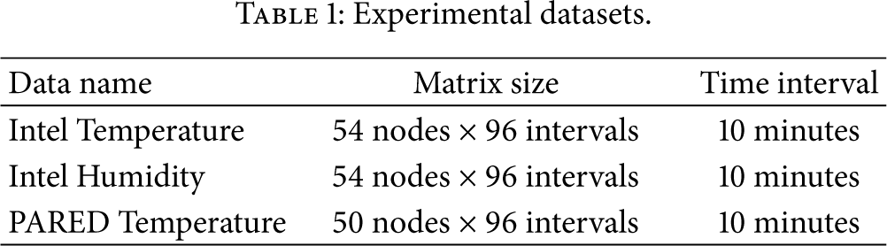
The first category of datasets is collected by 54 Mica2Dot nodes deployed in the Intel Berkeley Research Lab [17] between February 28 and April 5, 2004. The Mica2Dot node reports collected sensor data including humidity and temperature once every 30 seconds. However, we find that the raw dataset has considerable missing data. Therefore, we have rearranged the raw data (by changing the reporting interval from 30 seconds to 10 minutes) to avoid the missing data.

The second category of dataset consists of temperature readings, which are collected with a 10-minute interval by our own testbed, namely, PARED. PARED consists of 50 sensor nodes. More details about PARED can be found in [18].

4.2. Low-Rank Structure

We first examine the low-rank structure in WSN datasets using the Singular Value Decomposition (SVD). The environment matrix X can be decomposed into three matrices by SVD:

$$\begin{array}{cc}& X=U\Sigma V^T,\end{array}$$

(7)

where U is an $m\times m$ orthonormal matrix, V is an $n\times n$ orthonormal matrix, and Σ is an $m\times n$ diagonal matrix with singular values ${\sigma }_{\mathrm{1}},{\sigma }_{\mathrm{2}}\cdots {\sigma }_p$ sorted in a descending order $(p=\min (m,n))$ .

Because sensor readings in a WSN are spatiotemporal correlated, the environment matrix X would exhibit low-rank feature. More exactly, X should approximate to a low-rank matrix of rank r. So, the first r singular values will occupy the most energy of X. We use the following as the metric to examine the quality of the low-rank approximation:

$$\begin{array}{cc}& g\left(r\right)=\frac{{\sum }_{i=\mathrm{1}}^r{\sigma }_i}{{‖X‖}_{\ast }}=\frac{{\sum }_{i=\mathrm{1}}^r{\sigma }_i}{{\sum }_{i=\mathrm{1}}^p{\sigma }_i},\end{array}$$

(8)

where ${‖·‖}_{\ast }$ is the nuclear norm and ${‖X‖}_{\ast }={\sum }_{i=\mathrm{1}}^p‍{\sigma }_i$ .

Figure 1 shows the low-rank approximation quality of the three datasets. We found that the largest 10 singular values occupy the 93%–99% of the total energy, which suggests that the WSN datasets exhibit a good low-rank feature.

Figure 1

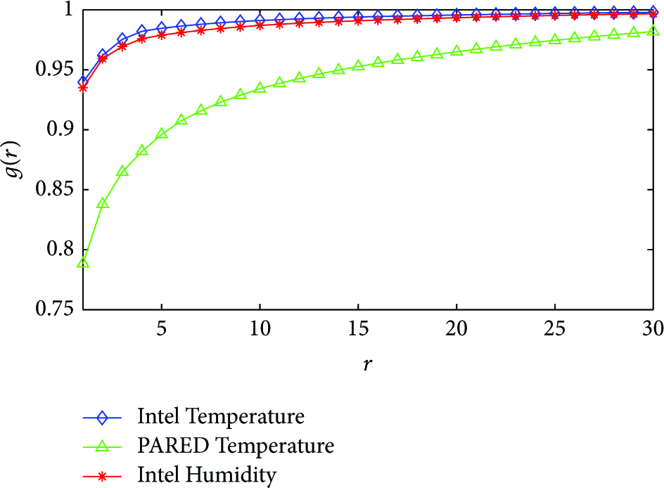
Low-rankness feature.

4.3. DCT Compactness

We also observed that the sensor readings in WSN exhibit DCT compactness feature. In other words, the first k DCT coefficients of the sensor vector ${\overrightarrow{x}}_i$ concentrate the most energy of ${\overrightarrow{x}}_i$ .

We first define D as the 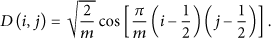$m\times m$ Discrete Cosine Transform Matrix:

$$\begin{array}{cc}& D\left(i,j\right)=\sqrt{\frac{\mathrm{2}}{m}}\cos \left[\frac{\pi }{m}\left(i-\frac{\mathrm{1}}{\mathrm{2}}\right)\left(j-\frac{\mathrm{1}}{\mathrm{2}}\right)\right].\end{array}$$

(9)

Then, the $m\times m$ orthonormal matrix D can be divided into two submatrices:

$$\begin{array}{cc}& D=\left[\begin{array}{c}{D}_{\mathrm{1}}\\ D_{\mathrm{2}}\end{array}\right],\end{array}$$

(10)

where $D_{\mathrm{1}}$ consists of the first k rows of D and $D_{\mathrm{2}}$ consists of the last $m-k$ rows of D.

Therefore, if the first k DCT coefficients occupy the most energy of ${\overrightarrow{x}}_i$ , we will have ${‖D_{\mathrm{1}}{\overrightarrow{x}}_i‖}_2/{‖{\overrightarrow{x}}_i‖}_2\approx \mathrm{1}$ and ${‖D_{\mathrm{2}}{\overrightarrow{x}}_i‖}_2/{‖{\overrightarrow{x}}_i‖}_2\approx \mathrm{0}$ . Similarly, for the matrix form, we will have ${‖D_{\mathrm{1}}X‖}_F/{‖X‖}_F\approx \mathrm{1}$ and ${‖D_{\mathrm{2}}X‖}_F/{‖X‖}_F\approx \mathrm{0}$ , where ${‖\ast ‖}_F$ is the Frobenius norm with ${‖X‖}_F=\sqrt{{\sum }_{i,j}‍X(i,j{)}^{\mathrm{2}}}$ . So, we use the following function to examine the DCT compactness feature:

$$\begin{array}{cc}& h\left(k\right)=\frac{{‖D_{\mathrm{1}}X‖}_F}{{‖X‖}_F}.\end{array}$$

(11)

From Figure 2, we can see that the first 10 DCT coefficients concentrate $\mathrm{99}\%$ of the total energy, which suggests that these WSN datasets exhibit a good DCT compactness feature.

Figure 2

DCT compactness feature.

5. Algorithm

In this section, we proposed a novel matrix completion algorithm, namely, DCT Regularized Matrix Completion (DRMC), to solve the data recovery problem in WSN data gathering. DRMC takes full advantage of the low-rankness and DCT compactness features to improve the recovery accuracy.

5.1. Utilization of Low-Rankness

As mentioned before in Section 3, the goal of the recovery problem is to estimate X from only a fraction of known entries. According to [10], we can recover X by solving the following rank optimization problem if X is a low-rank matrix:

$$\begin{array}{cc}& \mathrm{m}\mathrm{i}\mathrm{n}\mathrm{i}\mathrm{m}\mathrm{i}\mathrm{z}\mathrm{e}\hspace{1em}\mathrm{r}\mathrm{a}\mathrm{n}\mathrm{k}\left(X\right)\\ \mathrm{s}\mathrm{u}\mathrm{b}\mathrm{j}\mathrm{e}\mathrm{c}\mathrm{t}\hspace{0.17em}\hspace{0.17em}\mathrm{t}\mathrm{o}\hspace{1em}M\circ X=Y.\end{array}$$

(12)

However, the rank minimization problem (12) is NP-hard and is not solvable in polynomial time. Since the nuclear norm is the optimal convex approximation of the rank function, a reasonable solution is to solve a convex relaxation problem with the rank function replaced by the nuclear norm:

$$\begin{array}{cc}& \mathrm{m}\mathrm{i}\mathrm{n}\mathrm{i}\mathrm{m}\mathrm{i}\mathrm{z}\mathrm{e}\hspace{1em}{‖X‖}_{\ast }\\ \mathrm{s}\mathrm{u}\mathrm{b}\mathrm{j}\mathrm{e}\mathrm{c}\mathrm{t}\hspace{0.17em}\hspace{0.17em}\mathrm{t}\mathrm{o}\hspace{1em}M\circ X=Y.\end{array}$$

(13)

However, in a more realistic occasion, the environment matrix X is not an exactly low-rank matrix. There may not exist low-rank matrices that exactly satisfy the constraints in problem (13). So, we converted the constrained optimization problem (13) into the following nuclear norm regularized optimization problem:

$$\begin{array}{cc}& \mathrm{m}\mathrm{i}\mathrm{n}\mathrm{i}\mathrm{m}\mathrm{i}\mathrm{z}\mathrm{e}\hspace{0.17em}\hspace{0.17em}\frac{\mathrm{1}}{\mathrm{2}}{‖M\circ X-Y‖}_F^{\mathrm{2}}+\lambda {‖X‖}_{\ast },\end{array}$$

(14)

where $\lambda >\mathrm{0}$ is the nuclear regularization parameter.

5.2. Utilization of DCT Compactness

Though we can estimate X by solving the optimization problem (14), it will overfit to the known entries of X when the sampling rate is low, which will lead to large recovery error in the estimation of the missing entries.

Therefore, to reduce the overfitting in (14), we exploit the DCT compactness feature of the sensor data. As mentioned in Section 4.3, ${‖D_{\mathrm{2}}X‖}_F/{‖X‖}_F\approx \mathrm{0}$ . So, we added ${‖D_{\mathrm{2}}X‖}_F$ as the DCT regularization term to (14), and finally, we obtain the following optimization problem:

$$\begin{array}{cc}& \mathrm{m}\mathrm{i}\mathrm{n}\mathrm{i}\mathrm{m}\mathrm{i}\mathrm{z}\mathrm{e}\hspace{0.17em}\hspace{0.17em}\frac{\mathrm{1}}{\mathrm{2}}{‖M\circ X-Y‖}_F^{\mathrm{2}}+\lambda {‖X‖}_{\ast }+\mu {‖D_{\mathrm{2}}X‖}_F^{\mathrm{2}},\end{array}$$

(15)

where μ is the DCT regularization parameter.

5.3. The DRMC Algorithm

We present the DRMC algorithm by solving the optimization problem in (15). The pseudocode is shown in Algorithm 1. Next, we will describe the design of DRMC in details.

Algorithm 1: DRMC algorithm.

Input:

  $$Y\in {\mathbb{R}}^{m\times n}$$ : collected data matrix

  $$M\in {\mathbb{R}}^{m\times n}$$ : sampling matrix

  $$\stackrel{-}{\lambda }$$ : nuclear norm regularization parameter

 μ: DCT regularization parameter

Output:

  $$\widehat{X}\in {\mathbb{R}}^{m\times n}$$ : reconstructed environment matrix

Main procedure:

( $$\mathit{1}$$ )     $$L\leftarrow \mathrm{1}+\mathrm{2}\mu$$ ;

( $$\mathit{2}$$ )     $$X_{\text{old}}\leftarrow \mathbf{0}$$ ; $$X_{\text{new}}\leftarrow \mathbf{0}$$ ;

( $$\mathit{3}$$ )    Select $${\lambda }_{\mathrm{1}}>{\lambda }_{\mathrm{2}}>\cdots >{\lambda }_K=\stackrel{-}{\lambda }$$

( $$\mathit{4}$$ )    for   $$\lambda ={\lambda }_{\mathrm{1}},{\lambda }_{\mathrm{2}},\dots ,{\lambda }_K$$   do

( $$\mathit{5}$$ )      $$t_{\text{old}}\leftarrow \mathrm{1}$$ ; $$t_{\text{new}}\leftarrow \mathrm{1}$$ ;

( $$\mathit{6}$$ )     repeat

( $$\mathit{7}$$ )       $$Z⟵X_{\text{new}}+\frac{t_{\text{old}}-\mathrm{1}}{t_{\text{new}}}\left(X_{\text{new}}-X_{\text{old}}\right)$$ ;

( $$\mathit{8}$$ )       $$X_{\text{old}}\leftarrow X_{\text{new}}$$ ;

( $$\mathit{9}$$ )       $$G\leftarrow Z-L^{-\mathrm{1}}(M\circ Z-Y+\mathrm{2}\mu D_{\mathrm{2}}^T{D}_{\mathrm{2}}Z)$$ ;

( $$\mathit{1}$$ 0)    $$X_{\text{new}}\leftarrow S_{\lambda L^{-\mathrm{1}}}(G)$$ ;

( $$\mathit{11}$$ )    $$t_{\text{old}}\leftarrow t_{\text{new}}$$ ;

( $$\mathit{12}$$ )    $$t_{\mathrm{n}\mathrm{e}\mathrm{w}}⟵\frac{\mathrm{1}+\sqrt{\mathrm{1}+\mathrm{4}{t}_{\text{old}}^{\mathrm{2}}}}{\mathrm{2}}$$ ;

( $$\mathit{13}$$ )  until   $${‖X_{\text{new}}-X_{\text{old}}‖}_F/{‖X_{\text{old}}‖}_F<ϵ$$

( $$\mathit{14}$$ ) end for

( $$\mathit{15}$$ ) $$\widehat{X}\leftarrow X_{\text{new}}$$ ;

( $$\mathit{16}$$ ) return   $$\widehat{X}$$

The object function in (15) can be rewritten into the following form:

$$\begin{array}{cc}& F\left(X\right)≔f\left(X\right)+P\left(X\right),\end{array}$$

(16)

with

$$\begin{array}{cc}& f\left(X\right)=\frac{\mathrm{1}}{\mathrm{2}}{‖M\circ X-Y‖}_F^{\mathrm{2}}+\mu {‖D_{\mathrm{2}}X‖}_F^{\mathrm{2}},\end{array}$$

(17)

$$\begin{array}{cc}& P\left(X\right)=\lambda {‖X‖}_{\ast }.\end{array}$$

(18)

Note that $P(X)$ is a proper, convex, lower semicontinuous (lsc) [19] function but it is nonsmooth, while $f(X)$ is a convex smooth function and is continuously differentiable, with

$$\begin{array}{cc}& \nabla f\left(X\right)=\left(M\circ X-Y\right)+\mathrm{2}\mu D_{\mathrm{2}}^T{D}_{\mathrm{2}}X.\end{array}$$

(19)

Furthermore, $\nabla f(X)$ is Lipschitz continuous with a positive constant L:

$$\begin{array}{l}{‖\nabla f\left(X_{\mathrm{1}}\right)-\nabla f\left(X_{\mathrm{2}}\right)‖}_F\le L{‖X_{\mathrm{1}}-X_{\mathrm{2}}‖}_F,\hfill \\ \forall X_{\mathrm{1}},X_{\mathrm{2}}\in \mathrm{dom}P,\hfill \end{array}$$

(20)

where $\mathrm{dom}P=\{X\hspace{0.17em}|\hspace{0.17em}P(X)<\infty \}$ . Proposition 2 indicates that the Lipschitz constant of $f(X)$ is $L=\mathrm{1}+\mathrm{2}\mu$ .

Since $P(X)$ is nonsmooth, it is difficult to directly minimize the objective function $F(X)$ . Instead, we choose to iteratively minimize a sequence of quadratic approximations of $F(X)$ , which is an effective way to minimize the unconstrained nonsmooth convex function [20–22]. The quadratic approximation of $F(·)$ at point Z is defined as the following:

$$\begin{array}{l}{Q}_L\left(X,Z\right)≔f\left(Z\right)+〈\nabla f\left(Z\right),X-Z〉+\frac{L}{\mathrm{2}}{‖X-Z‖}_F^{\mathrm{2}}\hfill \\ +P\left(X\right).\hfill \end{array}$$

(21)

And the objective variable $X_{\mathrm{n}\mathrm{e}\mathrm{w}}$ is repeatedly updated to the minimizer of $Q_L(X,Z)$ , until ${‖X_{\mathrm{n}\mathrm{e}\mathrm{w}}-X_{\mathrm{o}\mathrm{l}\mathrm{d}}‖}_F/{‖X_{\mathrm{o}\mathrm{l}\mathrm{d}}‖}_F<ϵ$ . The convergence of such iterative process is well studied in [21].

We then introduce an auxiliary variable G to minimize $Q_L(X,Z)$ . As suggested by Proposition 5, we can minimize $Q_L(X,Z)$ using the singular value shrinkage operator defined in (26). Thus, we have $X_{\mathrm{n}\mathrm{e}\mathrm{w}}=S_{\lambda L^{-\mathrm{1}}}(G)$ .

What is more, we consider a warm-start technique for the nuclear regularization parameter λ. Rather than remaining unchanged, λ is monotonically decreasing in the iterative process. The nuclear regularization parameter λ starts with an initial value ${\lambda }_{\mathrm{1}}$ and gradually declines to $\bar{\lambda }$ , forming a sequence of ${\lambda }_{\mathrm{1}}>{\lambda }_{\mathrm{2}}>\cdots >{\lambda }_K,\hspace{0.17em}\hspace{0.17em}({\lambda }_K=\bar{\lambda })$ .

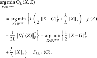
Lemma 1.

$D_{\mathrm{2}}$ is defined as in (10). Then, one has

$$\begin{array}{cc}& {‖D_{\mathrm{2}}^T{D}_{\mathrm{2}}X‖}_F\le {‖X‖}_F,\forall X\in {\mathbb{R}}^{m\times n}.\end{array}$$

(22)

Proof.

Since D is orthonormal, $D_{\mathrm{2}}{D}_{\mathrm{2}}^T=I,{‖DX‖}_F={‖X‖}_F$ .

And note that ${‖X‖}_F=\sqrt{Tr(X^{T}X)}$ , then we can obtain

$$\begin{array}{l}{‖D_{\mathrm{2}}^T{D}_{\mathrm{2}}X‖}_F=\sqrt{Tr\left(X^T{D}_{\mathrm{2}}^T{D}_{\mathrm{2}}{D}_{\mathrm{2}}^T{D}_{\mathrm{2}}X\right)}\hfill \\ =\sqrt{Tr\left(X^T{D}_{\mathrm{2}}^T{D}_{\mathrm{2}}X\right)}={‖D_{\mathrm{2}}X‖}_F\hfill \\ \le {‖DX‖}_F={‖X‖}_F.\hfill \end{array}$$

(23)

Proposition 2.

Assume that $f(X)$ is defined as (17); then, $f(X)$ is Lipschitz continuous with

$$\begin{array}{cc}& L=\mathrm{1}+\mathrm{2}\mu .\end{array}$$

(24)

Proof.

Note that ${‖M\circ X‖}_F\le {‖X‖}_F$ , and by using the Lemma 1, we obtain that

$$\begin{array}{l}{‖\nabla f\left(X_{\mathrm{1}}\right)-\nabla f\left(X_{\mathrm{2}}\right)‖}_F\hfill \\ ={‖M\circ \left(X_{\mathrm{1}}-X_{\mathrm{2}}\right)+\mathrm{2}\mu D_{\mathrm{2}}^T{D}_{\mathrm{2}}\left(X_{\mathrm{1}}-X_{\mathrm{2}}\right)‖}_F\hfill \\ \le {‖M\circ \left(X_{\mathrm{1}}-X_{\mathrm{2}}\right)‖}_F+\mathrm{2}\mu {‖D_{\mathrm{2}}^T{D}_{\mathrm{2}}\left(X_{\mathrm{1}}-X_{\mathrm{2}}\right)‖}_F\hfill \\ \le {‖X_{\mathrm{1}}-X_{\mathrm{2}}‖}_F+\mathrm{2}\mu {‖X_{\mathrm{1}}-X_{\mathrm{2}}‖}_F\hfill \\ =\left(\mathrm{1}+\mathrm{2}\mu \right){‖X_{\mathrm{1}}-X_{\mathrm{2}}‖}_F.\hfill \end{array}$$

(25)

Definition 3.

Decompose the matrix $X\in {\mathbb{R}}^{m\times n}$ of rank r by SVD: $X=U\Sigma V^T$ , where $U\in {\mathbb{R}}^{m\times r}$ and $V\in {\mathbb{R}}^{n\times r}$ are orthonormal matrices and $\Sigma =\mathrm{d}\mathrm{i}\mathrm{a}\mathrm{g}(\{{\sigma }_i{\}}_{\mathrm{1}\le i\le r})$ . Define the singular value shrinkage operator [23] $S_{\lambda }$ as follows:

$$\begin{array}{cc}& S_{\lambda }\left(X\right)=U{S}_{\lambda }\left(\Sigma \right)V^T,\\ S_{\lambda }\left(\Sigma \right)=\mathrm{d}\mathrm{i}\mathrm{a}\mathrm{g}\left({\left\{{\left({\sigma }_i-\lambda \right)}_{+}\right\}}_{\mathrm{1}\le i\le r}\right),\end{array}$$

(26)

where $t_{+}$ is the positive part of t, $t_{+}=\mathrm{m}\mathrm{a}\mathrm{x}(\mathrm{0},t)$ .

Lemma 4.

Let $G\in {\mathbb{R}}^{m\times n}$ . Then,

$$\begin{array}{cc}& S_{\lambda }\left(G\right)\equiv \underset{X\in {\mathbb{R}}^{m\times n}}{\mathrm{a}\mathrm{r}\mathrm{g}\hspace{0.17em}\mathrm{m}\mathrm{i}\mathrm{n}}\left\{\frac{\mathrm{1}}{\mathrm{2}}{‖X-G‖}_F^{\mathrm{2}}+\lambda {‖X‖}_{\ast }\right\},\end{array}$$

(27)

where $S_{\lambda }(G)$ is the singular value shrinkage operator of G.

Proof.

The proof of Lemma 4 can be found in [23].

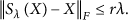
Proposition 5.

Let 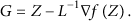$Z\in {\mathbb{R}}^{m\times n}$ and $P(X)=\lambda {‖X‖}_{\ast }$ . Assume that $f(X)$ is Lipschitz continuous and define $G\in {\mathbb{R}}^{m\times n}$ with

$$\begin{array}{cc}& G=Z-L^{-\mathrm{1}}\nabla f\left(Z\right).\end{array}$$

(28)

Then, one has

$$\begin{array}{cc}& \underset{X\in {\mathbb{R}}^{m\times n}}{\mathrm{a}\mathrm{r}\mathrm{g}\hspace{0.17em}\mathrm{m}\mathrm{i}\mathrm{n}}\hspace{0.17em}{Q}_L\left(X,Z\right)=S_{\lambda L^{-\mathrm{1}}}\left(G\right).\end{array}$$

(29)

Proof.

Consider

$$\begin{array}{l}{Q}_L\left(X,Z\right)=f\left(Z\right)+〈\nabla f\left(Z\right),X-Z〉+\frac{L}{\mathrm{2}}{‖X-Z‖}_F^{\mathrm{2}}\hfill \\ +P\left(X\right)\hfill \\ =f\left(Z\right)+〈\nabla f\left(Z\right),X-Z〉+\frac{L}{\mathrm{2}}{‖X-Z‖}_F^{\mathrm{2}}\hfill \\ +\lambda {‖X‖}_{\ast }\hfill \\ =\frac{L}{\mathrm{2}}{‖X-Z-\frac{\mathrm{1}}{L}\nabla f\left(Z\right)‖}_F^{\mathrm{2}}+\lambda {‖X‖}_{\ast }\hfill \\ +f\left(Z\right)-\frac{\mathrm{1}}{\mathrm{2}L}{‖\nabla f\left(Z\right)‖}_F^{\mathrm{2}}\hfill \\ =L\left\{\frac{\mathrm{1}}{\mathrm{2}}{‖X-G‖}_F^{\mathrm{2}}+\frac{\lambda }{L}{‖X‖}_{\ast }\right\}+f\left(Z\right)\hfill \\ -\frac{\mathrm{1}}{\mathrm{2}L}{‖\nabla f\left(Z\right)‖}_F^{\mathrm{2}}.\hfill \end{array}$$

(30)

Thus, combined with Lemma 4, we can obtain that

$$\begin{array}{l}\underset{X\in {\mathbb{R}}^{m\times n}}{\mathrm{a}\mathrm{r}\mathrm{g}\hspace{0.17em}\mathrm{m}\mathrm{i}\mathrm{n}}\hspace{0.17em}{Q}_L\left(X,Z\right)\hfill \\ =\underset{X\in {\mathbb{R}}^{m\times n}}{\mathrm{a}\mathrm{r}\mathrm{g}\hspace{0.17em}\mathrm{m}\mathrm{i}\mathrm{n}}\left\{L\left(\frac{\mathrm{1}}{\mathrm{2}}{‖X-G‖}_F^{\mathrm{2}}+\frac{\lambda }{L}{‖X‖}_{\ast }\right)+f\left(Z\right)\right\}\hfill \\ -\frac{\mathrm{1}}{\mathrm{2}L}{‖\nabla f\left(Z\right)‖}_F^{\mathrm{2}}=\underset{X\in {\mathbb{R}}^{m\times n}}{\mathrm{a}\mathrm{r}\mathrm{g}\hspace{0.17em}\mathrm{m}\mathrm{i}\mathrm{n}}\left\{\frac{\mathrm{1}}{\mathrm{2}}{‖X-G‖}_F^{\mathrm{2}}\right\}\hfill \\ +\frac{\lambda }{L}{‖X‖}_{\ast }=S_{\lambda L^{-\mathrm{1}}}\left(G.\right)\hfill \end{array}$$

(31)

6. Complexity Analysis

In this section, we discuss the time complexity of the proposed algorithm.

After analyzing the steps in Algorithm 1, we find that the most computationally intensive step is the singular value shrinkage operation that performs SVD on G, which dominates the computational complexity of this algorithm. The time complexity of SVD for an $m\times n$ matrix is $O(m{n}^{\mathrm{2}})$ [24]. And for any $ϵ>\mathrm{0}$ , the iterative process in Algorithm 1 will terminate in $O(\sqrt{L/ϵ})$ iterations with an ϵ-optimal solution [21, 25]. Consequently, the time complexity of our algorithm is $O(K\sqrt{L/ϵ}m{n}^{\mathrm{2}})$ .

We can further decrease the time complexity of the DRMC algorithm by applying Partial Reorthogonalization Package (PROPACK) [26] in the singular value shrinkage operation. PROPACK uses the Lanczos method [24] to compute only a partial SVD of G. However, it cannot a priori compute singular values that are greater than $\lambda /L$ . Hence, we need to predetermine the number of singular values to be computed (denoted as $s{v}_i$ ) at the beginning of the ith iteration, and PROPACK can then compute the $s{v}_i$ largest singular values and corresponding singular vectors. We adopt the prediction rule proposed in [27]:

$$\begin{array}{cc}& s{v}_{i+\mathrm{1}}=\left\{\begin{array}{cc}sv{p}_i+\mathrm{1},\hfill & \mathrm{i}\mathrm{f}\hspace{0.17em}\hspace{0.17em}sv{p}_i<s{v}_i.\hfill \\ \min \left\{sv{p}_i+\mathrm{10},m,n\right\},\hfill & \mathrm{i}\mathrm{f}\hspace{0.17em}\hspace{0.17em}sv{p}_i=s{v}_i,\hfill \end{array}\right.\end{array}$$

(32)

where $s{v}_i$ is the predicted number of singular values, $sv{p}_i$ is the actual number of singular values that are larger than $\lambda /L$ , and $s{v}_{\mathrm{0}}=\mathrm{10}$ .

The time complexity of the Lanczos method is $O(rmn)$ for $m\times n$ matrix with rank of r [24]. Therefore, the time complexity of DRMC algorithm is $O(K\sqrt{L/ϵ}rmn)$ if PROPACK is used. For fixed number of iterations, the complexity of DRMC can be simplified as $O(rmn)$ , while the state-of-the-art matrix completion based methods [11–13] require a complexity of $O(r^{\mathrm{2}}mn)$ . So, DRMC is more computationally efficient.

7. Error Analysis

In this section, we analyze the recovery error of the DRMC algorithm and present a theoretical upper bound.

Before starting the analysis, we first introduce some assumptions and lemmas.

Assumption 6.

The original data matrix X can be approximated by the first k DCT coefficients, with approximation error ξ:

$$\begin{array}{cc}& \xi ={‖X-D_{\mathrm{1}}^T{D}_{\mathrm{1}}X‖}_F={‖D_{\mathrm{2}}^T{D}_{\mathrm{2}}X‖}_F.\end{array}$$

(33)

Assumption 7.

Let $\mathcal{A}:{\mathbb{R}}^{m\times n}\to {\mathbb{R}}^{m\times n}$ be the linear operator defined as

$$\begin{array}{cc}& \mathcal{A}\left(X\right)=\mathrm{2}\mu L^{-\mathrm{1}}{D}_{\mathrm{2}}^T{D}_{\mathrm{2}}X+L^{-\mathrm{1}}M\circ X\end{array}$$

(34)

and $\mathcal{I}$ be the identity operator.

Then, there exists a constant $\mathrm{0}\le \eta <\mathrm{1}$ , such that

$$\begin{array}{cc}& \underset{\mathcal{A}\left(X\right)\ne \mathrm{0},{‖X‖}_F=\mathrm{1}}{\sup }{‖\left(\mathcal{I}-\mathcal{A}\right)\left(X\right)‖}_F\le \eta .\end{array}$$

(35)

Lemma 8.

Suppose that $S_{\lambda }$ is the singular value shrinkage operator; then,

$$\begin{array}{l}{‖S_{\lambda }\left(X_{\mathrm{1}}\right)-S_{\lambda }\left(X_{\mathrm{2}}\right)‖}_F\le {‖X_{\mathrm{1}}-X_{\mathrm{2}}‖}_F,\hfill \\ \forall X_{\mathrm{1}},X_{\mathrm{2}}\in {\mathbb{R}}^{m\times n}.\hfill \end{array}$$

(36)

Proof.

The detailed proof of Lemma 8 can be found in [28].

Lemma 9.

Suppose that $X\in {\mathbb{R}}^{m\times n}$ with rank of r; then,

$$\begin{array}{cc}& {‖S_{\lambda }\left(X\right)-X‖}_F\le r\lambda .\end{array}$$

(37)

Proof.

Consider

$$\begin{array}{l}{‖S_{\lambda }\left(X\right)-X‖}_F={‖U\left(S_{\lambda }\left(\Sigma \right)-\Sigma \right)V^T‖}_F\hfill \\ ={‖U\left(\Sigma -S_{\lambda }\left(\Sigma \right)\right)V^T‖}_F\hfill \\ ={‖U\left(\mathrm{diag}\left({\left\{{\sigma }_i-{\left({\sigma }_i-\lambda \right)}_{+}\right\}}_{\mathrm{1}\le i\le r}\right)\right)V^T‖}_F\hfill \\ ={‖U\mathrm{d}\mathrm{i}\mathrm{a}\mathrm{g}\left({\left\{d_i\right\}}_{\mathrm{1}\le i\le r}\right)V^T‖}_F=\sqrt{{\displaystyle \sum }_{i=\mathrm{1}}^r{d_i}^{\mathrm{2}}},\hfill \end{array}$$

(38)

where

$$\begin{array}{cc}& d_i=\left\{\begin{array}{cc}\lambda ,\hfill & \mathrm{i}\mathrm{f}\hspace{0.17em}\hspace{0.17em}{\sigma }_i\ge \lambda ;\hfill \\ {\sigma }_i,\hfill & \mathrm{i}\mathrm{f}\hspace{0.17em}\hspace{0.17em}{\sigma }_i<\lambda .\hfill \end{array}\right.\end{array}$$

(39)

Therefore, we have

$$\begin{array}{cc}& {‖S_{\lambda }\left(X\right)-X‖}_F\le r\lambda .\end{array}$$

(40)

The upper bound of the recovery error is then given in the following theorem.

Theorem 10.

Suppose that $\widehat{X}$ is the estimate of X obtained by the DRMC algorithm; then, one has

$$\begin{array}{cc}& {‖\widehat{X}-X‖}_F\le \frac{r\bar{\lambda }+\mathrm{2}\xi \mu }{\left(\mathrm{1}-\eta \right)\left(\mathrm{1}+\mathrm{2}\mu \right)}.\end{array}$$

(41)

Proof.

When the iterative process in Algorithm 1 has converged, 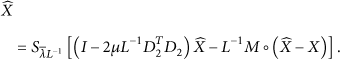$X_{\mathrm{n}\mathrm{e}\mathrm{w}}$ will be equal to $X_{\mathrm{o}\mathrm{l}\mathrm{d}}$ . Hence, $\widehat{X}$ will be the fixed point of the following:

$$\begin{array}{l}\widehat{X}\hfill \\ =S_{\bar{\lambda }{L}^{-\mathrm{1}}}\left[\left(I-\mathrm{2}\mu L^{-\mathrm{1}}{D}_{\mathrm{2}}^T{D}_{\mathrm{2}}\right)\widehat{X}-L^{-\mathrm{1}}M\circ \left(\widehat{X}-X\right)\right].\hfill \end{array}$$

(42)

Therefore, we have

$$\begin{array}{l}{\Vert \widehat{X}-X\Vert }_F=\Vert S_{\bar{\lambda }{L}^{-1}}[\left(I-2\mu L^{-1}{D}_2^T{D}_2\right)\widehat{X}-L^{-1}M\hfill \\ \hspace{0.17em}\hspace{0.17em}\hspace{0.17em}\circ \left(\widehat{X}-X\right)]-{X\Vert }_F=\Vert S_{\bar{\lambda }{L}^{-1}}[\left(I-2\mu L^{-1}{D}_2^T{D}_2\right)\widehat{X}\hfill \\ \hspace{0.17em}\hspace{0.17em}\hspace{0.17em}-L^{-1}M\circ \left(\widehat{X}-X\right)]\hfill \\ \hspace{0.17em}\hspace{0.17em}\hspace{0.17em}-S_{\bar{\lambda }{L}^{-1}}\left[\left(I-2\mu L^{-1}{D}_2^T{D}_2\right)X\right]\hfill \\ \hspace{0.17em}\hspace{0.17em}\hspace{0.17em}{+S_{\bar{\lambda }{L}^{-1}}\left[\left(I-2\mu L^{-1}{D}_2^T{D}_2\right)X\right]-X\Vert }_F\hfill \\ \hspace{0.17em}\hspace{0.17em}\hspace{0.17em}\le \Vert S_{\bar{\lambda }{L}^{-1}}[\left(I-2\mu L^{-1}{D}_2^T{D}_2\right)\widehat{X}-L^{-1}M\hfill \\ \hspace{0.17em}\hspace{0.17em}{\hspace{0.17em}\circ \left(\widehat{X}-X\right)]-S_{\bar{\lambda }{L}^{-1}}\left[\left(I-2\mu L^{-1}{D}_2^T{D}_2\right)X\right]\Vert }_F\hfill \\ \hspace{0.17em}\hspace{0.17em}\hspace{0.17em}+\Vert S_{\bar{\lambda }{L}^{-1}}(X)-X{\Vert }_F+2\mu L^{-1}{\Vert D_2^T{D}_{2}X\Vert }_F.\hfill \end{array}$$

(43)

Combining (43) and Lemma 8, we have

$$\begin{array}{l}{‖\widehat{X}-X‖}_F\hfill \\ \le {‖\left(I-\mathrm{2}\mu L^{-\mathrm{1}}{D}_{\mathrm{2}}^T{D}_{\mathrm{2}}\right)\left(\widehat{X}-X\right)-L^{-\mathrm{1}}M\circ \left(\widehat{X}-X\right)‖}_F\hfill \\ +{‖S_{\bar{\lambda }{L}^{-\mathrm{1}}}\left(X\right)-X‖}_F+\mathrm{2}\mu L^{-\mathrm{1}}{‖D_{\mathrm{2}}^T{D}_{\mathrm{2}}X‖}_F\hfill \\ ={‖\left(\mathcal{I}-\mathcal{A}\right)\left(\widehat{X}-X\right)‖}_F+{‖S_{\bar{\lambda }{L}^{-\mathrm{1}}}\left(X\right)-X‖}_F\hfill \\ +\mathrm{2}\mu L^{-\mathrm{1}}{‖D_{\mathrm{2}}^T{D}_{\mathrm{2}}X‖}_F,\hfill \end{array}$$

(44)

where $\mathcal{I}$ is the identity operator and $\mathcal{A}$ is the operator defined in (34).

Then, applying Assumption 6 and Lemma 9 to (44), we have

$$\begin{array}{cc}& {‖\widehat{X}-X‖}_F\le {‖\left(\mathcal{I}-\mathcal{A}\right)\left(\widehat{X}-X\right)‖}_F+\bar{\lambda }{L}^{-\mathrm{1}}r+\mathrm{2}\mu L^{-\mathrm{1}}\xi .\end{array}$$

(45)

Combining Assumption 7, (24), and (45), we finally obtain the following error bound:

$$\begin{array}{cc}& {‖\widehat{X}-X‖}_F\le \frac{r\bar{\lambda }+\mathrm{2}\xi \mu }{\left(\mathrm{1}-\eta \right)L}=\frac{r\bar{\lambda }+\mathrm{2}\xi \mu }{\left(\mathrm{1}-\eta \right)\left(\mathrm{1}+\mathrm{2}\mu \right)}.\end{array}$$

(46)

Let E represent the upper bound of the recovery error. Then, according to Theorem 10, $E=(r\bar{\lambda }+\mathrm{2}\xi \mu )/(\mathrm{1}-\eta )(\mathrm{1}+\mathrm{2}\mu )$ . Note that $E(\bar{\lambda })$ is an increasing function of $\bar{\lambda }$ . So, we expect the actual recovery error of the DRMC algorithm to increase with $\bar{\lambda }$ , which is confirmed later by simulation results in Section 8.3.

8. Evaluation

We designed a data gathering scheme based on the proposed DRMC algorithm. The data gathering procedure is similar to [11]. Firstly, sink node broadcasts a sampling rate to all sensor nodes. Secondly, each sensor node randomly and independently decides whether to forward its readings to the sink according to the sampling rate. Finally, the sink node collects the incomplete data matrix and uses DRMC to retrieve the missing data. After implementing this data gathering scheme by Matlab, we carried out extensive experiments on three real-world datasets (as shown in Table 1) to evaluate the effectiveness of DRMC.

8.1. Baseline Methods

We select two state-of-the-art methods to compare with DRMC. The first method is Compressive Sensing (CS). We choose the DCT matrix defined in (9) to serve as the orthonormal basis in CS. The second method is Spatiotemporal Compressive Data Collection (STCDG). The parameters of STCDG are set to $\lambda =\mathrm{0.5}$ , $r=\mathrm{10}$ . Note that since our earlier work, namely, DCT-RPMC, depends on historical data while the proposed algorithm does not, we do not select DCT-RPMC as the baseline method.

8.2. Recovery Accuracy

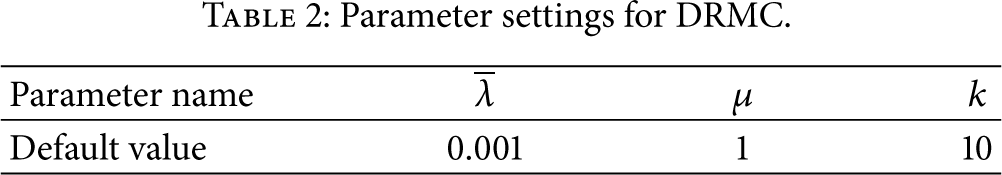
Firstly, we compared the recovery accuracy of the proposed algorithm with two baseline methods described above. The parameters of DRMC are listed in Table 2.

Table 2

Parameter settings for DRMC.

Parameter name	$$\stackrel{-}{\lambda }$$	μ	k
Default value	0.001	1	10

Simulation experiments are carried out on three real-world datasets. Each simulation is conducted for 100 independent trials. The recovery errors are computed according to (6) and are averaged over the 100 trials.

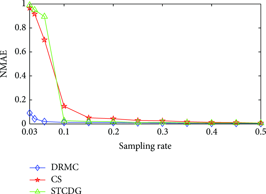
Comparison results are shown in Figures 3–5. For experiments on Intel Temperature Trace, all methods achieve nearly the same recovery accuracy when the sampling rate is high. When the sampling rate is below a certain value ( $\tau <\mathrm{0.1}$ ), recovery performance of baseline methods deteriorates quickly, while DRMC still achieves a good recovery accuracy. When the sampling rate is as low as 0.03, which means 97% of data loss, DRMC can reconstruct the lost data with recovery error less than 10%, while recovery error of CS and STCDG is close to 100%.

Figure 3

Recovery accuracy on Intel Temperature Trace.

Figure 4

Recovery accuracy on Intel Humidity Trace.

Figure 5

Recovery accuracy on PARED Temperature Trace.

Comparison results on Intel Humidity Trace are very similar to that on Intel Temperature Trace. Recovery error of DRMC is about 9% when the sampling rate is 0.03, which is noticeably better than that of baseline methods.

For experiments on PARED Temperature Trace, DRMC still outperforms baseline methods for low sampling rate. The recovery error of DRMC is about $\mathrm{16}\%$ when the sampling rate is 0.03, which is slightly worse than that on other two traces. This is because the low-rankness and DCT compactness features of PARED Temperature are not as good as that of other two traces, as shown in Figures 1 and 2.

8.3. Parameter Settings

The DRMC algorithm depends on several input parameters. Clearly, the choice of these parameters will affect the recovery performance of DRMC. In this subsection, we discuss how to choose the parameters for DRMC.

The nuclear norm regularization parameter λ is an important parameter to ensure the low-rank feature of the reconstructed data matrix. In DRMC, we adopted a warm-start strategy for λ, in which λ is linearly reduced from ${\lambda }_{\mathrm{1}}$ to ${\lambda }_K$ . In the implementation, ${\lambda }_{\mathrm{1}}=\mathrm{10}\bar{\lambda }+\mathrm{1}$ , ${\lambda }_K=\bar{\lambda }$ , and $K=\mathrm{20}$ . We tested DRMC on a range of values of $\bar{\lambda }$ to investigate how $\bar{\lambda }$ effects the performance of DRMC. Figure 6 shows the experimental results. The recovery errors of DRMC increase with $\bar{\lambda }$ , just as what we predicted in Section 7 by the theoretical error bound (41). Note that when $\bar{\lambda }<\mathrm{0.1}$ , the recovery performance of DRMC is not sensitive to $\bar{\lambda }$ . So, in practice, we just set it to a small enough value, $\bar{\lambda }=\mathrm{0.001}$ .

Figure 6

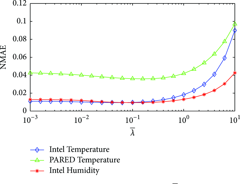
Effect of parameter $\bar{\lambda }$ .

Parameter μ is a regularization parameter that guarantees the DCT compactness feature of the recovered signal. Figure 7 shows the effects of μ on the recovery performance of DRMC. The recovery errors decline with μ and are stable when $\mu >\mathrm{0.1}$ . So, we choose to use $\mu =\mathrm{1}$ for our experiments.

Figure 7

Effect of parameter μ.

Recall that k represents the number of concentrated DCT coefficients. As discussed before in Section 4.3, the first 10 DCT coefficients concentrate 99% of the total energy. As expected, Figure 8 shows that the recovery errors are dropping fast with k and are stable when $k>\mathrm{10}$ . So, we choose to use $k=\mathrm{10}$ for our experiments. Note that the recovery errors are slightly increasing with the growth of k when $k>\mathrm{10}$ . We explain this by considering the extreme case when $k=m$ . If $k=m$ , $D_{\mathrm{1}}$ is equal to D. As a result, the DCT regularization term ${‖D_{\mathrm{2}}X‖}_F^2$ in (15) is automatically equal to zero. Therefore, the DCT compactness property of the sensory data is not utilized and the recovery errors will increase, just as the case in Figure 7 when $\mu =\mathrm{0}$ .

Figure 8

Effect of parameter k.

8.4. Energy Consumption and Network Lifespan

DRMC-based data gathering protocol is more energy efficient because it transmits less packets than the classic one (receiving and forwarding). As a result, DRMC-based protocol can save more energy and prolong the lifespan of wireless sensor networks. To verify this, simulation experiments are conducted and the simulation configuration is shown in Table 3.

Table 3

Simulation configuration for network lifespan.

Parameter name	Value
Number of nodes	1000
Initial energy	1 J
Sampling period	10 seconds
Data size	16 bits
$$E_{Tx}$$	100 nJ/bit
$$E_{Rx}$$	120 nJ/bit
$$E_{\text{Amp}}$$	0.01 nJ/(bit⋅m2)

In the simulation, sensor nodes are randomly deployed in a 500 m × 500 m area and the sink node is deployed in the center. Each sensor node is equipped with 1 J energy. To evaluate the energy consumption, we adopt the following energy model [29]:

$$\begin{array}{cc}& E_T\left(k,d\right)=\left\{\begin{array}{cc}\left(E_{Tx}+d^{\mathrm{2}}\times E_{\mathrm{A}\mathrm{m}\mathrm{p}}\right)\times k,\hfill & \mathrm{i}\mathrm{f}\hspace{0.17em}\hspace{0.17em}d<d_{\mathrm{T}\mathrm{h}\mathrm{r}\mathrm{e}\mathrm{s}},\hfill \\ \left(E_{Tx}+d^{\mathrm{4}}\times E_{\mathrm{A}\mathrm{m}\mathrm{p}}\right)\times k,\hfill & \mathrm{i}\mathrm{f}\hspace{0.17em}\hspace{0.17em}d\ge d_{\mathrm{T}\mathrm{h}\mathrm{r}\mathrm{e}\mathrm{s}},\hfill \end{array}\right.\\ E_R\left(k\right)=k{E}_{Rx}.\end{array}$$

(47)

$E_T(k,d)$ represents the energy consumption of transmitting k bits data with distance d. $E_R(k)$ denotes the energy consumption of receiving k bits data. $E_{Tx}$ is the energy consumed by the transmitting circuit to process 1 bit data. $E_{Rx}$ is the energy consumed by the receiving circuit to process 1 bit data. $E_{\mathrm{A}\mathrm{m}\mathrm{p}}$ is the energy consumed by power amplifying circuit.

Figure 9 demonstrates the network lifespan of DRMC-based protocol and other baseline protocols under different sampling rate. Note that the network lifespan is defined as the time when the first energy exhausted node appears. Apparently, the sampling rate does not play a role in the classic data gathering, since it directly transmits all data without compression. Therefore, the lifespan curve of the classic protocol in Figure 9 is a straight line. For the CS method, the smaller the sampling rate is, the less measurements are taken. And as shown in Figure 9, the lifespan of CS is decreasing with the sampling rate. However, when the sampling rate is above a certain value, the lifespan of CS is even worse than the classic one. The reason why CS performs badly for large sampling rate is well analyzed in [30]. Figure 9 shows that DRMC-based protocol achieves the best lifespan. Similarly, the lifespan of DRMC is decreasing with the sampling rate. When the sampling rate decreases to 1, DRMC-based protocol is equivalent to the classic protocol and the lifespan of DRMC is equal to the classic one. Note that the lifespan of STCDG is exactly the same as DRMC, because both of the two methods are based on matrix completion. The lifespan of DRMC is longer than CS because the sampling matrix in DRMC is much sparser than that in CS.

Figure 9

Relation of network lifespan to sampling rate.

9. Conclusion

In this paper, we studied the data gathering and reconstruction problem in WSNs. We modeled the problem as matrix completion problem and investigated the data features in real WSN datasets. Then, by taking advantage of the low-rankness and DCT compactness features in WSNs, we proposed a DCT Regularized Matrix Completion (DRMC) algorithm to reconstruct the missing data. The recovery error of DRMC is carefully analyzed and a theoretical error upper bound is presented. Experimental results show that DRMC outperforms state-of-the-art methods for low sampling rate and achieves a good recovery accuracy even if the sampling rate is very low.