Sage Journals: Discover world-class research

Abstract

A real-time indoor tracking system based on the Viterbi algorithm is developed. This Viterbi principle is used in combination with semantic data to improve the accuracy, that is, the environment of the object that is being tracked and a motion model. The starting point is a fingerprinting technique for which an advanced network planner is used to automatically construct the radio map, avoiding a time consuming measurement campaign. The developed algorithm was verified with simulations and with experiments in a building-wide testbed for sensor experiments, where a median accuracy below 2 m was obtained. Compared to a reference algorithm without Viterbi or semantic data, the results indicated a significant improvement: the mean accuracy and standard deviation improved by, respectively, 26.1% and 65.3%. Thereafter a sensitivity analysis was conducted to estimate the influence of node density, grid size, memory usage, and semantic data on the performance.

1. Introduction

Indoor localization and tracking systems have applications in many domains; think of the healthcare sector, industrial sector, cultural sector, and so forth. Examples of these applications are tracing of elderly, equipment tracking, and museum guidance. Indoor environments are complex and give rise to multipath and shadowing effects due to refraction, reflection, and scattering from walls and obstacles [1]. This results in localization systems which are often not sufficiently accurate. Current state-of-the-art localization systems try to improve the accuracy by using new technologies and more intelligent algorithms, such as ultrawideband (UWB), route constraints, and particle filters.

The focus of this work is on accurately tracking a real person through a building-wide environment in real-time while using the existing wireless sensor network (WSN) or wireless local area network (WLAN) infrastructure to avoid the need for dedicated hardware. The novelties of this paper are the real-time usage of the Viterbi principle and semantic data, a network planner for the fingerprinting technique (avoiding an expensive and time consuming measurement campaign, which makes the localization system very fast to deploy), an extended experimental validation and simulation, and a sensitivity analysis in which the influence of the tracking algorithm parameters on the performance is estimated.

The remainder of this paper is organized as follows: Section 2 describes related work, Section 3 presents the developed tracking algorithm and its optimizations, and Section 4 describes the configuration. The simulation and experimental validation are described in Sections 5 and 6, respectively. Section 7 presents the sensitivity analysis and Section 8 concludes the paper.

2. Related Work

Localization systems can be distinguished from each other in multiple ways [2, 3]. These systems can be either active or passive. With passive localization, also known as device-free localization, the moving object is not actively participating in the localization process [4–7]. The position is estimated based on changes in the environment, which are in turn caused by the presence and movement of the entity that is being tracked. This is interesting for noncooperative localization like intrusion detection or wildlife monitoring. Most localization systems are active and, in this case, the object that is being tracked is equipped with an active tag. This tag sends out beacons that are received by a fixed infrastructure. The infrastructure consists of fixed nodes or access points (APs), forming the wireless network. There are also localization systems that do not depend on a fixed infrastructure but instead use a signal of opportunity (SoOP). These SoOPs are signals that are already present in the environment of interest (e.g., FM radio signals [8], acoustic background noise [9], or the earth magnetic field [10]). The active localization systems can be further divided based on the used signal: global positioning system (GPS), global system for mobile communications (GSM), ultrasound, infrared (IR), radio-frequency identification (RFID), optical, ZigBee, WiFi, or UWB. GPS signals are mostly used for outdoor localization because of the global availability and sufficient accuracy. Because of the disability to penetrate most building materials, these GPS signals are not suited for indoor localization. Optical systems have the disadvantage of becoming unusable in situations with limited visibility like smoke or fire. Localization systems making use of ultrasound, IR, or RFID are purpose-built systems, which are hard to implement on a larger scale and can be expensive. With UWB technology, centimeter level accuracies are possible because of the fine temporal resolution provided by the large bandwidth. Disadvantages are the higher operational costs and the limited coverage range which makes them more suited for short-range applications. ZigBee and WiFi are the two most used technologies in WSNs and WLANs. Both are widely deployed, which makes them suitable for localization with negligible overhead and without expensive hardware costs. Besides differentiation on the used signal, another distinction of localization systems can be made, based on the used ranging technique. Angle of Arrival (AoA) [11], Time Difference of Arrival (TDoA) [12], and Received Signal Strength Indicator (RSSI) [13] are common techniques that are mostly used in combination with triangulation, trilateration, and RSSI fingerprinting, respectively. The advantage of the latter is that most devices are already capable of measuring the RSSI, whereas AoA or TDoA systems require specialized hardware (directional antennas for AoA and clock synchronization between the receiving nodes for TDoA). A completely different approach to tracking is pedestrian dead reckoning (PDR); this technique predicts the current position based on a previous position and measurements from inertial motion sensors. Because this technique works without a wireless signal, no infrastructure or connectivity is needed [14–16]. The biggest challenge of PDR is how to cope with the accumulating error because of the typical noisy measurement data from these inertial sensors. Disadvantages are the start position and orientation of the inertial sensor unit that must be known in advance and that need to be consistent with respect to the object that is being tracked. These disadvantages can be solved by merging PDR with an external measurement source like, for example, WLAN measurements but then the advantages of not depending on any infrastructure disappear.

In [17] an RSSI fingerprinting technique with GSM signals and route constraints is used to locate a moving vehicle. Beside the fact that it is aimed at outdoor localization, the difference from our approach is that measurement data is needed to train a Hidden Markov Model (HMM). In [18] a location prediction method based on path planning is presented. The path planning model is used to constrain the movement trajectory of the mobile target. This is used for location prediction which is weighted with a maximum-likelihood estimation (MLE). The paths on which a target can move are very restricted and the authors only used simulations to verify their approach. The average localization error depends on the transmission range and average connectivity of the anchor nodes and lies between 1.5 m and 3 m. In [19] a localization algorithm based on maximum a posteriori probability (MAP) and RSSI ranging is proposed. The goal is to locate the sensor nodes, whereas in our approach the location of the fixed nodes is known in advance and the goal is to track a mobile user. Furthermore, a performance evaluation was carried out but only with simulations, no practical experiments were performed. In [20] a real-time particle filter for 2D and 3D hybrid indoor positioning is presented. It uses floor plan restrictions and a particle smoother to correct previous positions. The obtained accuracy is 2 m with the particle filter and 1.4 m with the smoother. The difference with our approach is that, besides WLAN based position measurements, it also depends on a hand-held inertial sensor unit and a barometer. Also, the learning phase depends on training data for the positioning with WLAN, which implies a measurement campaign. In [8] a positioning system is proposed, based on FM broadcast as a signal of opportunity. The advantage of FM signals is the higher stability due to the longer wavelength compared to WiFi; disadvantages are the lower accuracy and the need for dedicated hardware. It combines both deterministic and probabilistic techniques and the obtained accuracy is 2.5 m when 150 reference points are used (which is time consuming). In [21] a grid based filter and Viterbi algorithm are used as the central processor for data fusion to estimate the location. Motion dynamics information (MDI) measured with smartphone sensors is used to calculate the state transition probabilities. In our proposed algorithm we use the environmental data and do not rely on MDI data. In [22], a WiFi positioning method to locate mobile terminals is presented. A hybrid model based on the RADAR [23] model and Friis-Based Calibrated Model (FBCM) is suggested. The RADAR model is improved by taking topological elements into account. Therefore, the neighborhood of each point needs to be given. In our approach, only a floor plan needs to be provided to automatically take into account the environment and more extensive experiments were conducted.

3. Tracking Algorithm

3.1. RSSI Fingerprinting with Advanced Network Planner

The starting point of the developed tracking algorithm is an RSSI fingerprinting technique [24]. This technique differs from other localization systems because the location is not determined based on estimated distances between transmitter and receiver. Instead it consists of two phases: an offline training phase and an online localization phase.

During the offline phase a radio map of the area of interest is constructed. This radio map contains the signal strength values at every possible grid point for all fixed APs or ZigBee sensors. These signal strength values and radio map are also called reference fingerprints and fingerprint database, respectively. The grid points on the floor plan represent the positions where the object that is being tracked can be located. The density of these grid points is determined by the resolution or grid size; this is the distance between two neighboring grid points. The reference fingerprints can be calculated with a theoretical model or obtained through a measurement campaign. During the online phase, these reference fingerprints are compared to the measured signal strengths to estimate the user's location.

We used an advanced network planner to construct the fingerprint database, avoiding an expensive and time consuming measurement campaign (WHIPP tool [25]). This approach results in a slightly reduced accuracy but allows an immediate deployment. The only prerequisite to generate the fingerprint database for a certain building is to draw its floor plan with the right materials in the WHIPP tool. Most common materials are already available in the tool: brick, drywall, wood, glass, and metal, both in thin and in thick format. Due to the changing nature of furniture and other nonstatic objects, they are not included. The tool uses an advanced heuristic path loss model which is constructed based on PL samples collected in an office building and was verified in three other types of buildings: a retirement home, a congress center, and an arts center. Without any additional measurements or tuning, the predictions were also excellent. Three contributions are taken into account to calculate the total path loss (from which the received signal strength can be deducted (see Section 4.1)): the sum of the distance loss along the path, the total wall loss along the path, and the interaction loss along the path:

\begin{array}{l} {PL}_{ref} = \underset{distance loss}{\underset{︸}{{PL}_{0} + 10 n \log_{10} (\frac{d}{d_{0}})}} + \underset{cumulated wall loss}{\underset{︸}{\sum_{i} L_{W_{i}}}} \\ + \underset{interaction loss}{\underset{︸}{\sum_{j} L_{B_{j}}}} (dB) . \end{array}

(1)

PL_ref (dB) is the total path loss calculated with the WHIPP tool, ${PL}_{0}$ (dB) is the path loss at a reference distance $d_{0}$ (m), n (-) is the path loss exponent, and d (m) is the distance along the path between transmitter and receiver. The first two terms represent the path loss due to the traveled distance (distance loss), the third term (cumulated wall loss) is the sum of all wall losses $L_{W_{i}}$ when a signal propagates through a wall $W_{i}$ , and the fourth term (interaction loss) takes into account the cumulated losses $L_{B_{j}}$ caused by all propagation direction changes $B_{j}$ of the propagation path from transmitter to receiver.

3.2. Viterbi Algorithm and Semantic Data

The developed tracking system intelligently exploits the Viterbi principle [26]. This dynamic programming algorithm is used to determine the most likely sequence of hidden states, called the Viterbi path, resulting in the sequence of observed events. In this paper, we interpret the states as real locations on a floor plan, to apply this technique on a tracking algorithm. Then, this principle comes down to determining the most likely sequence of positions instead of only the most likely current position. In the remainder of this paper we will use the term path for a sequence of positions. During the online phase, all possible paths are stored and each path has an associated cost. This cost is defined as the sum of mean square errors (MSE) between measurements and reference fingerprints. At each time step, all costs are calculated and used as decision metric to determine the most likely path:

\begin{matrix} {MSE}_{i, t} = \frac{1}{N} \sum_{n = 1}^{N} {(RSSI_{meas}_{n, t} - RSSI_{ref}_{n, t, i})}^{2}, \\ {Cost}_{i, T} = \sum_{t = 1}^{T} {MSE}_{i, t} . \end{matrix}

(2)

${MSE}_{i, t}$ is the mean square error of path i at time step t, N is the number of APs that measure the RSSI from the user, $RSSI_{meas}_{n, t}$ is the RSSI measurement at time step t from AP n, and $RSSI_{ref}_{n, t, i}$ is the reference RSSI value from AP n for the grid point along path i at time step t, calculated with the WHIPP tool. ${Cost}_{i, T}$ is the associated cost of the ith path stored in memory at time step T and T is the number of time steps that went by since the tracking began. The last position of the path with the lowest associated cost is taken as most likely current location.

Our algorithm is not recursive in the strictest sense; that is, the function to determine the location is not applied within its own definition. But the algorithm is also not restarted every time a measurement is received. The paths and their associated costs from a previous iteration serve as input to the current iteration, along with the new measurements. After every location update (processing of these new measurements) a fixed number of paths are kept in memory (e.g., 1000). Previous time steps are used and represented by the paths which are kept in memory. To apply the Viterbi principle in a useful manner (improve the accuracy), we have to restrict the number of allowed transitions between two grid points. Therefore, we use semantic data: the environment of the object that is being tracked and a motion model. In Figure 1 an example is given to illustrate this principle. First, the environment is modeled by the same floor plan used in Section 3.1 to generate the fingerprint database. The WHIPP tool [25] generates the grid points on a room level basis and the location of the doors is used to indicate positions where the user can leave a room. A grid transition through each door is ensured by adding additional grid points in the middle of each door to the generated grid. To facilitate an easy transition, grid points on both sides of a door (within a certain distance, e.g., 1 m) are linked, alerting the tracking algorithm of a possible transition. In this way it is assured that no walls are crossed. By collecting all grid points between which a transition of realistic distance is possible in separate lists, the need for geometric intersection during the online phase is alleviated, which is computationally more efficient. Second, the motion model sets a maximum speed limit, ensuring that no unrealistically large distances are traveled within a given time frame. Overall, this leads to realistic and physically possible paths (see Figure 1). The pseudocode of the tracking system can be found in Algorithm 1.

Algorithm 1: Pseudocode tracking system.

Data: read new measurements collected by fixed APs

for all paths p in memory do

$l p$ = last position of p;

$c o s t$ = current cost of p;

$c p s$ = all candidate positions given $l p$ and semantic data;

if $l p$ is near a door then

add candidate positions near other side of this door to $c p s$ ;

end

for all candidate positions $c p$ in $c p s$ do

$m s e$ = mean square error between measurements and reference values of $c p$ ;

$n e w C o s t$ = $c o s t$ + $m s e$ ;

update p: save $c p$ and $n e w C o s t$ with link to p;

end

retain X paths with lowest costs;

$m l t$ = most likely trajectory (path with lowest cost);

estimated current location = last position of $m l t$ ;

wait for new measurements;

Figure 1

Semantic data taken into account.

In summary, the developed system is based on an RSSI fingerprinting technique which uses an advanced network planner to construct the radio map and uses the Viterbi principle and semantic data as optimizations. To the best of the author's knowledge this is the first tracking algorithm that uses this combination of techniques and optimizations. It is easily deployed, works in real-time, and is accurate for tracking in a building-wide environment.

3.3. Initial Position

Because the most likely sequence of positions is determined and the allowed transitions between two positions are restricted, the developed tracking algorithm is sensitive to a wrong starting position. One could start off in the wrong room, which implies a certain recovery time before predictions can be accurate again, because walls cannot be crossed. To counteract this, additional possible starting positions are added as soon as the tracking begins. These additional starting positions are located on circles around the best initial prediction and there are eight such positions per circle (see Figure 2). This method takes two arguments: levels and inter distance; levels is the number of circles that are added and inter distance is the distance between these circles. In all experiments levels was set to 5 and inter distance to 1 m.

Figure 2

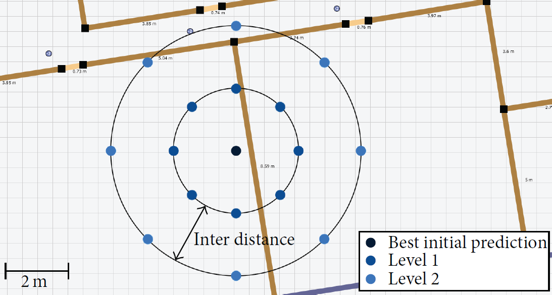
Additional starting positions.

This technique allows the algorithm to easily correct itself by switching to another path when new measurements suggest being located inside a different room. Hence the developed system is robust against a wrong starting position and does not need information about this position in advance, like, for example, pedestrian dead reckoning.

4. Configuration

4.1. Measurement and Simulation Setup

The measurements are conducted on a generic wireless testbed for sensor experiments (w-iLab.t [27]), located on the third floor of a modern office building in Ghent which measures 90 m by 17 m (displayed in Figure 3). It consists of several computer classes, offices, and meeting rooms. The core consists of concrete walls (gray walls in Figure 3(d)), the inner structure is movable and made of layered drywall (brown walls in Figure 3(d)), the doors are made of wood (yellow walls in Figure 3(d)), and the outside of the building consists of windows with metal blinds (blue walls in Figure 3(d)).

Figure 3

Measurements.

The fixed infrastructure is a testbed which consists of 57 sensor nodes and an equal amount of WiFi nodes that were installed at a height of 2.5 m (these are the blue dots in Figure 3(d)).

Two mobile nodes were used: a TMote Sky node [28] which uses ZigBee and a WiFi node, both fed by an external battery of 19 Volt (see Figure 3(a)). Both mobile nodes have a transmission rate of 10 packets/s and are operating in the 2.4 GHz frequency band. They have a bandwidth of 2 MHz and 20 MHz, respectively, and both have an external antenna with a gain of 5 dBi.

The RSSI values, measured by the fixed APs, are used to estimate the location but the fingerprint database consists of path loss values, calculated with the WHIPP tool (see Section 3.1). A quick calibration was needed to determine the shift between both: on four different locations a broadcast of 30 seconds was performed. The average difference was used as shift between the RSSI and the path loss values (which we assume to be fixed). This was once done for ZigBee and once for WiFi.

Nine test trajectories were used to evaluate our developed tracking algorithm. The simulation and experimental validation used the same trajectories, so we could easily compare both results with each other (see Section 7.1). These nine test trajectories had an average length of 87 m and were conducted in different areas of the building, by a person who walked at constant speed. The mobile nodes were hand-carried at a height of approximately 1.5 m, as far as possible from the body. The average walking speed was 1.10 m/s (about 4 km/h) which is a normal velocity for an indoor environment. Figure 3(d) shows three such trajectories in red, green, and black. The other six trajectories are similar but pass through different rooms.

4.2. Tracking Algorithm Settings

The used settings of the developed tracking algorithm can be found in Table 1. The maximum speed is fixed at 2 m/s and the sample rate is set to 1 sample/s which means, in this case, that we average the RSSI values of 10 packets because the mobile nodes have a transmission rate of 10 packets/s. The parameter memory in Table 1 represents how many paths are retained in memory at each time step. When set to 1000, we update all paths present in memory and we retain the 1000 best paths (i.e., with the lowest associated cost). The impact of this parameter on the calculation time is studied in Section 7.3. The grid size determines the resolution of possible positions on the floor plan where a person can be located; this is set to 0.5 m (an example of such a grid can be seen in Figure 2). The influence of this parameter is investigated in Section 7.2. The node density determines how many of the 57 fixed nodes are used in an experiment (blue dots in Figure 3(d)). As the current goal is achieving a high accuracy, this parameter is set to the maximum value. In Section 7.1 the impact of the node density is studied; this is important because in a realistic environment this node density will typically be much lower. On average, 25 out of 57 fixed nodes received the packets from the mobile node. At each time step, we only used the 10 strongest AP measurements (if available) to estimate the new location because increasing this number did not further improve the performance but only adds to the calculation time.

Table 1

Settings.

Setting	Value
Assumed maximum speed	2 m/s
Sample rate	1 sample/s
Memory	1000 paths
Grid size	0.5 m
Node density	57 nodes

4.3. Evaluation Metrics

To estimate the performance improvement when using the Viterbi principle and semantic data, we used a basic tracking algorithm as reference. This basic algorithm depends only on the RSSI fingerprinting technique from Section 2 and makes no usage of the Viterbi principle or semantic data from Section 3.2. For fair comparison, the basic algorithm does make use of the same fingerprint database (constructed with the advanced path loss model). In Section 7.4 the influence of this model is studied by comparing the results when a free-space model is used to construct the fingerprint database.

The developed algorithm has two outputs: Viterbi Current and Viterbi. The former works in real-time because it uses only the available information at the present time (current and past measurements) to estimate the location. The latter allows estimated locations from the past to be corrected by future measurements. In other words, Viterbi is the most likely path, given all the measurements. This is interesting for applications where a small delay is allowed or real-time is not required, for example, modeling or analyzing pedestrian and traffic flows.

The mean ( $μ_{E}$ ), standard deviation ( $σ_{E}$ ), median ( $P_{50}$ ), and 95th percentile value ( $P_{95}$ ) of the error were chosen as evaluation metrics. The error is defined as the Euclidean distance (in meters) between the predicted and the true position. In the remainder of this paper we will use the term accuracy instead of error. To determine the exact location of these true positions we assumed a constant walking speed; that is, the true positions are equally spread along a trajectory.

5. Simulations

5.1. Test Trajectories

To simulate real measurements, we add Gaussian noise with zero mean and a configurable standard deviation to the reference fingerprints generated with the WHIPP tool [25] ( $RSSI_ref$ in (2)) and use these as input for the tracking algorithms. In Figure 4 an example test trajectory (red) and the reconstruction (black) with both algorithms are shown. The standard deviation of the added Gaussian noise was set to 5 dB (we denote this as noise level) and both algorithms have processed the same input. As expected, the reconstructed path with the developed algorithm is realistic and physically possible, whereas in the basic algorithm some walls are crossed and impossibly large traveled distances are present.

Figure 4

Reconstruction of a test trajectory by (a) the basic and (b) the developed algorithm.

5.2. Influence of Noise Level

In this section the influence of an increasing noise level is evaluated. The impact on the performance of both algorithms is studied for four types of node density: sparse, normal, dense, and very dense. These node densities use, respectively, 5, 10, 20, and 57 fixed nodes for a surface of 90 m by 17 m or 1530 m² (see Figure 3(d)). Next, the accuracy is calculated for an increasing noise level (0–20 dB). In Figure 5, the mean accuracy $μ_{E}$ is plotted as a function of the added noise level; the error bars indicate the standard deviation $σ_{E}$ of this accuracy. Each simulation was repeated five times and $μ_{E}$ and $σ_{E}$ were averaged over the results of the nine test trajectories.

Figure 5

Influence of noise for various node densities (simulation).

Figure 5 shows that the developed Viterbi algorithm always outperforms the basic one, in terms of both mean accuracy and standard deviation. The absolute difference in mean accuracy between Viterbi and Basic decreases as node density increases: for a noise level of 10 dB these differences are 6.27 m, 4.17 m, 2.39 m, and 1.01 m for the four node densities, respectively. This is not a disadvantage as most buildings are not equipped with a dense wireless network; in practice this is rather the opposite. The relative improvement from Viterbi compared to Basic varies between a factor 2 and factor 3 for noise levels around 10 dB. There are two remarks: we assumed that the standard deviation of the measurement noise is equal for all measurements and that every fixed AP receives all packets sent by the mobile node, independently of the traveled distance. In practice, these two assumptions will not hold. However, both tracking algorithms have to process the same input, so the comparison remains valid.

6. Experimental Validation

In this section, the performance evaluation is based on the results obtained with the measurements conducted by a person who hand-carried the mobile ZigBee or WiFi node.

6.1. ZigBee

The results with the ZigBee node are averaged over all nine test trajectories and can be found in Table 2.

Table 2

Performance comparison.

Algorithm →		Basic	Viterbi Current	Viterbi
ZigBee	Mean [m]	3.06	2.54	2.26
	Standard deviation [m]	4.04	1.7	1.4
	Median [m]	2.3	2.14	1.99
	95th percentile [m]	7.34	5.87	5.0

WiFi	Mean [m]	3.61	3.02	2.86
	Standard deviation [m]	2.66	1.93	1.61
	Median [m]	3.09	2.65	2.59
	95th percentile [m]	7.55	6.21	6.05

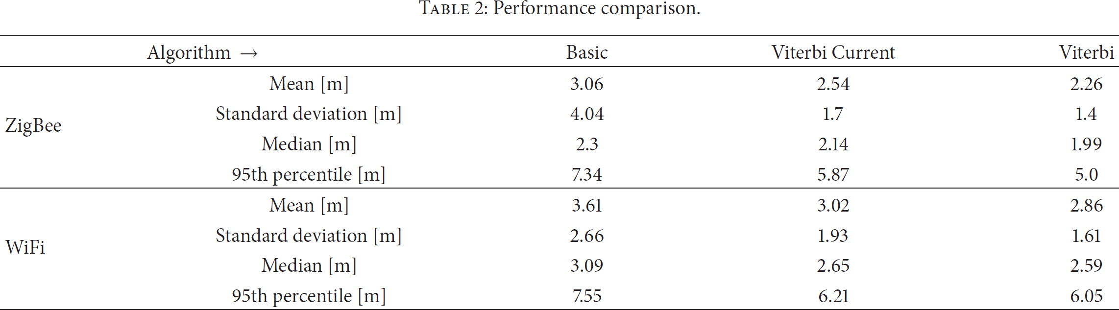
Table 2 shows that the median accuracy and standard deviation are below 2 m with Viterbi. Overall, the developed Viterbi algorithms always outperform the basic one. In particular the standard deviation and 95th percentile values are significantly reduced. The relative improvement in mean accuracy and standard deviation is 17% and 58% for Viterbi Current and 26% and 65% for Viterbi, respectively.

6.2. WiFi

Besides the ZigBee node, three test trajectories were investigated with the WiFi node. Because of the higher maximum transmit power, more fixed nodes received the packets from this mobile node (on average 40 out of 57 fixed nodes). This time, we used the 20 strongest AP measurements to estimate the location, for the same reason as with the ZigBee node (see Section 4.2). The other settings were the same as in Table 1 and the results can be found in Table 2. Again, the developed Viterbi algorithms perform better with improvements up to 39.5% in standard deviation. For ZigBee, more accurate results were obtained because, compared to the used ZigBee channel, there was more interference on the used WiFi channel. We used WiFi channel 1 (2412 MHz with a bandwidth of 20 MHz) and ZigBee channel 26 (2480 MHz with a bandwidth of 2 MHz), and some of the APs for regular wireless traffic also used WiFi channel 1.

7. Sensitivity Analysis

In this section a sensitivity analysis is conducted, based on the measurements from the experimental validation. This is important to estimate the influence of the tracking algorithm parameters on the performance (e.g., accuracy and execution time). Unless stated otherwise, the settings from Table 1 are used and the results are averaged over all nine trajectories, conducted with the ZigBee node. We will investigate node density, grid size, memory usage, and so forth.

7.1. Node Density

The majority of testbeds used for testing a new localization system have a very high node or AP density. In a typical environment this node density is typically much lower. The recommended node density for a wireless network infrastructure will depend on several factors, for example, the number of users, required bandwidth, and type of building, whereas the most important factor for a localization system will be the required accuracy. Cisco recommends a node density between 0.0015 APs/m² and 0.0043 APs/m² for their Cisco 1000 series lightweight access point [29]. The test environment has a surface area of 1530 m², which results in 7 APs for a node density of 0.0043 APs/m². The used testbed is equipped with 57 nodes, which leaves us many possibilities to investigate the performance from sparse to very dense networks. Four scenarios are considered (5, 10, 20, and 57 nodes as in Section 5.2). The mean accuracy ( $μ_{E}$ ) and standard deviation ( $σ_{E}$ ) are summarized in Table 3.

Table 3

Performance for different node densities.

Algorithm →			Basic		Viterbi Current		Viterbi
Scenario ↓	Number of nodes	Nodes/m²	$μ_{E}$ [m]	$σ_{E}$ [m]	$μ_{E}$ [m]	$σ_{E}$ [m]	$μ_{E}$ [m]	$σ_{E}$ [m]
Sparse	5	0.0033	8.3	11.89	6.04	9.1	5.11	7.81
Normal	10	0.0065	6.58	11.41	3.76	2.58	3.26	2.24
Dense	20	0.013	4.78	8.34	3.2	2.1	2.7	1.72
Very dense	57	0.037	3.06	4.04	2.54	1.7	2.26	1.4

It is clear that the developed algorithm shows already acceptable results in a network with normal node density. More specifically, Viterbi Current and Viterbi perform 2.82 m and 3.32 m better compared to the basic algorithm in terms of mean accuracy (an improvement of 42.9% and 50.5%, resp.). This is due to many bad predictions of the basic algorithm (see high $σ_{E}$ ), which worsen the mean accuracy a lot. When we compare these results with those from the simulation (Section 5), we observe similar mean accuracies for a noise level around 10 dBm but higher standard deviations, caused by measurement outliers. These can be due to body influence.

7.2. Grid Size

The grid size determines the resolution of the possible positions on the floor plan where a person can be located. A lower grid size has the benefit of a finer resolution at the cost of a higher execution time or needed computational power because the search space is larger. In this section, the influence of this parameter on the performance of the developed algorithm is investigated for four different grid sizes (see Table 4).

Table 4

Performance for different grid resolutions.

Algorithm →	Viterbi Current				Viterbi
Grid size [m] ↓	$μ_{E}$ [m]	$σ_{E}$ [m]	$P_{50}$ [m]	$P_{95}$ [m]	$μ_{E}$ [m]	$σ_{E}$ [m]	$P_{50}$ [m]	$P_{95}$ [m]
0.2	2.6	1.74	2.22	6.24	2.34	1.47	2.02	5.38
0.5	2.54	1.7	2.14	5.87	2.26	1.4	1.99	5.0
1	2.64	1.81	2.15	6.28	2.22	1.42	1.96	5.09
2	3.01	2.12	2.52	7.28	2.82	1.89	2.4	6.64

Grid sizes of 0.2 m, 0.5 m, and 1 m yield similar performance: a mean accuracy of a bit more than 2 m, standard deviation of 1.5 m, median accuracy just below 2 m, and a 95th percentile value around 5 m. This is because as soon as the grid size is small compared to the achieved median accuracy, the performance will not further improve by further reducing the grid size. Thus, a grid size of 1 m is recommended when time or computational power is limited because a smaller grid size increases the execution time and the number of calculations of both the offline and online phase.

7.3. Execution Time

The average time needed to calculate one location update will determine the ability for real-time usage and will depend not only on the available computational power but also on some parameters related to the developed tracking system. In particular, the grid size and the number of paths stored in memory will have an influence on the execution time. In Figure 6, this execution time is plotted as a function of the number of paths in memory, for four different grid sizes (logarithmic scale). The solid lines are the execution times with the developed algorithm and the dotted lines with the basic algorithm. We take 1000 paths as upper limit because there is no further improvement in accuracy if more than 1000 paths are stored; for the larger grid sizes even less paths are needed. The experiments are run on a desktop computer with an Intel Core i7 3.40 GHz processor, 8.00 GB DDR3-SDRAM, and 64-bit operating system.

Figure 6

Average execution time to calculate one location update for different grid sizes (solid line: developed algorithm, dotted line: basic algorithm).

The time needed to calculate one location update increases more or less exponentially with the number of paths that are stored and updated at every time step and quadratically with a smaller grid size because halving the grid size results in four times as many grid points (on a two-dimensional floor plan). The basic algorithm does not depend on this number of paths; therefore we see a nearly constant line in Figure 6. For a low number of paths, the developed system performs faster than the basic one because, to determine the most likely position, basic will try every grid point on the floor plan and Viterbi will try only those centered around a previous position (due to the motion model). We can also see that for a grid size of 2 m the execution time remains the same for 500 to 1000 paths because, along the nine trajectories, the maximum possible paths remained below 500. The maximum delay is about 1 s when we use 1000 paths and a grid size of 20 cm. For real-time localization applications it is better to use a grid size of 1 m and 100 paths. Then it takes only 1.5 ms to calculate a location update while there is almost no loss in accuracy; this leaves some margin to run in real-time on devices with less computational power.

7.4. Path Loss Model

Until now we have always used the advanced heuristic path loss model from the network planner (WHIPP) to construct our fingerprint database (see Section 3.1). In Table 5 the performance with a free-space path loss model is compared to the one with WHIPP. We used the following formula:

\begin{matrix} {PL}_{free-space} = 20 \log_{10} (\frac{4 π}{c} d f) (dB) . \end{matrix}

(3)

Table 5

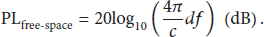
Influence of used path loss model.

Algorithm ↓	Path loss model ↓	$μ_{E}$ [m]	$σ_{E}$ [m]	$P_{50}$ [m]	$P_{95}$ [m]
Basic	Free-space	3.35	3.43	2.68	7.98
Basic	WHIPP	3.06	4.04	2.3	7.34
Viterbi	Free-space	2.62	1.6	2.36	5.82
Viterbi	WHIPP	2.26	1.4	1.99	5.0

$PL_{free-space}$ (dB) is the total path loss calculated with the free-space path loss model, f (Hz) is the signal frequency (2.4 GHz), c (m/s) is the speed of light ( $3 \cdot 10^{8}$ m/s), and d (m) is the distance between transmitter and receiver. To allow an entirely fair comparison with the WHIPP model, the free-space model was calibrated with the same four measurements from Section 4.1.

Except for the standard deviation with the basic algorithm, the results with the WHIPP model always outperform the ones with a free-space path loss model. Compared to Basic + free-space, the mean accuracy improves by 32.5%, the standard deviation by 59.1%, the median by 25.7%, and the 95th percentile value by 37.3% when using the developed tracking algorithm and the network planner (Viterbi + WHIPP).

7.5. Semantic Data

In this section the added value of the semantic data (environmental data and motion model) is investigated. In Table 6 four types of semantic data while using the Viterbi algorithm are considered.

Table 6

Influence of semantic data.

Semantic data ↓	$μ_{E}$ [m]	$σ_{E}$ [m]	$P_{50}$ [m]	$P_{95}$ [m]
None	3.06	4.04	2.3	7.34
Environmental data	2.71	2.59	2.17	6.62
Motion model	2.27	1.42	2.03	5.05
Both	2.26	1.4	1.99	5.0

When no semantic data is taken into account, the Viterbi principle has no added value because any transition between two positions is possible and we have the same result as with the basic algorithm. Using the environmental data (e.g., no wall crossing and leaving a room through the doors) gives a small improvement but the motion model (limitation on the assumed maximum speed) results in the largest improvement. Using both still yields the best results but the additional value is limited because there are only a few room changes over the course of an entire trajectory. Most of the time, a user is walking in a room or in the hall way.

7.6. Viterbi Principle

In this section the number of previous time steps (in other words, the number of estimated previous positions), used to estimate the new location, is weighed against the accuracy. When less time steps have to be taken into account, less calculations and paths are needed. This is important for situations where resources (e.g., computational power or memory) are limited. In Figure 7 the four metrics are plotted as a function of this parameter. To see the benefit more clearly, we used a normal node density (10 nodes or 0.0065 nodes/m²).

Figure 7

Influence of the number of previous time steps taken into account to estimate the new location on the four metrics (in a normal node density).

Figure 7 shows that no further improvement in any of the four metrics is noticeable when nine or more previous time steps are taken into account. This also means that we can reduce our memory usage by only storing the measurement data from the last nine time steps.

8. Conclusion

In this paper, a real-time indoor tracking system based on the Viterbi algorithm and semantic data was presented. The system was evaluated by both simulations and an experimental validation in an office environment. In the simulations it was shown that the developed tracking system was more robust against RSSI prediction errors, especially for networks with smaller node densities. In the experimental validation, an average median accuracy of below 2 m was obtained. Compared to a basic RSSI fingerprinting technique, the predictions were more accurate in terms of mean and median accuracy and there was a huge improvement in standard deviation and 95th percentile value. More concrete, the mean accuracy improved by 26.14%, the standard deviation by 65.35%, the median by 13.48%, and the 95th percentile value by 31.88%. It was shown that the node density has a major impact on the accuracy; with the developed tracking algorithm acceptable results could be obtained in normal node densities (a mean accuracy of 3.26 m compared to 6.58 m with the basic algorithm). It was shown that the semantic data was necessary to exploit the Viterbi principle; in particular the motion model has a major influence. Compared to a free-space path loss model, the usage of the WHIPP tool to construct the fingerprint database improved the median accuracy of the developed Viterbi algorithm by 15.68%. The grid size and the number of used previous time steps, to estimate the new location, have a huge impact on the execution time, required computational power, and memory usage. This is important to work in real-time on low cost devices. Future work will include the simultaneous tracking of multiple people on multiple floors.

Footnotes

Conflict of Interests

The authors declare that there is no conflict of interests regarding the publication of this paper.

References

Hashemi

The indoor radio propagation channel

Proceedings of the IEEE 1993 81 7 943 968

10.1109/5.231342

2-s2.0-0027627694

Cheng

Zhang

Maple

A survey of localization in wireless sensor network

International Journal of Distributed Sensor Networks 2012 2012 12

962523

2-s2.0-84872123719

10.1155/2012/962523

Viani

Rocca

Oliveri

Trinchero

Massa

Localization, tracking, and imaging of targets in wireless sensor networks: an invited review

Radio Science 2011 46 5

10.1029/2010rs004561

2-s2.0-80052774797

Patwari

Wilson

RF sensor networks for device-free localization: measurements, models, and algorithms

Proceedings of the IEEE 2010 98 11 1961 1973

10.1109/jproc.2010.2052010

2-s2.0-77958152993

Wilson

Patwari

See-through walls: motion tracking using variance-based radio tomography networks

IEEE Transactions on Mobile Computing 2011 10 5 612 621

10.1109/tmc.2010.175

2-s2.0-79952925499

Seifeldin

Saeed

Kosba

A. E.

El-Keyi

Youssef

Nuzzer: a large-scale device-free passive localization system for wireless environments

IEEE Transactions on Mobile Computing 2013 12 7 1321 1334

10.1109/tmc.2012.106

2-s2.0-84878159171

Zhao

Patwari

Phillips

J. M.

Venkatasubramanian

Radio tomographic imaging and tracking of stationary and moving people via kernel distance

Proceedings of the 12th International Conference on Information Processing in Sensor Networks (IPSN '13)

April 2013

ACM

229 240

10.1145/2461381.2461410

2-s2.0-84876773592

Moghtadaiee

Dempster

A. G.

Indoor location fingerprinting using fm radio signals

IEEE Transactions on Broadcasting 2014 60 2 336 346

10.1109/tbc.2014.2322771

2-s2.0-84901102001

Tarzia

S. P.

Dinda

P. A.

Dick

R. P.

Memik

Indoor localization without infrastructure using the acoustic background spectrum

Proceedings of the 9th International Conference on Mobile Systems, Applications, and Services (MobiSys ′11)

July 2011

ACM

155 168

2-s2.0-79961086186

10.1145/1999995.2000011

10.

Chung

Donahoe

Schmandt

Kim

I.-J.

Razavai

Wiseman

Indoor location sensing using geo-magnetism

Proceedings of the 9th International Conference on Mobile Systems, Applications, and Services (MobiSys ′11)

July 2011

ACM

141 154

2-s2.0-79961084039

10.1145/1999995.2000010

11.

Elnahrawy

Austen-Francisco

Martin

R. P.

Adding angle of arrival modality to basic RSS location management techniques

Proceedings of the 2nd International Symposium on Wireless Pervasive Computing (ISWPC ′07)

February 2007

San Juan, Puerto Rico

IEEE

10.1109/iswpc.2007.342648

2-s2.0-34548120687

12.

Merhi

Elgamel

Bayoumi

M. A.

A lightweight collaborative fault tolerant target localization system for wireless sensor networks

IEEE Transactions on Mobile Computing 2009 8 12 1690 1704

10.1109/tmc.2009.81

2-s2.0-70350602616

13.

Zanca

Zorzi

Zanella

Zorzi

Experimental comparison of RSSI-based localization algorithms for indoor wireless sensor networks

Proceedings of the 3rd Workshop on Real-World Wireless Sensor Networks (REALWSN ′08)

April 2008

1 5

10.1145/1435473.1435475

2-s2.0-62949204512

14.

Constandache

Choudhury

R. R.

Rhee

Towards mobile phone localization without war-driving

Proceedings of the IEEE INFOCOM

March 2010

San Diego, Calif, USA

IEEE

1 9

2-s2.0-77953305134

10.1109/infcom.2010.5462058

15.

Wang

Sen

Elgohary

Farid

Youssef

Choudhury

R. R.

No need to war-drive: unsupervised indoor localization

Proceedings of the 10th International Conference on Mobile Systems, Applications, and Services (MobiSys '12)

June 2012

ACM

197 210

10.1145/2307636.2307655

2-s2.0-84864335859

16.

Alzantot

Youssef

UPTIME: ubiquitous pedestrian tracking using mobile phones

Proceedings of the IEEE Wireless Communications and Networking Conference (WCNC ′12)

April 2012

IEEE

3204 3209

10.1109/wcnc.2012.6214359

2-s2.0-84864331687

17.

Coleri Ergen

Tetikol

H. S.

Kontik

Sevlian

Rajagopal

Varaiya

RSSI-fingerprinting-based mobile phone localization with route constraints

IEEE Transactions on Vehicular Technology 2014 63 1 423 428

10.1109/TVT.2013.2274646

2-s2.0-84893372100

18.

Gao

Shi

Zhou

Wang

A location predicting method for indoor mobile target localization in wireless sensor networks

International Journal of Distributed Sensor Networks 2013 2013 11

949285

10.1155/2013/949285

2-s2.0-84876579719

19.

Xiang

Zhang

Mao

Feng

Localization algorithm based on maximum a posteriori in wireless sensor networks

International Journal of Distributed Sensor Networks 2012 2012 7

260302

10.1155/2012/260302

2-s2.0-84862961907

20.

Nurminen

Ristimaki

Ali-Loytty

Piché

Particle filter and smoother for indoor localization

Proceedings of the International Conference on Indoor Positioning and Indoor Navigation (IPIN ′13)

October 2013

Montbeliard, France

1 10

10.1109/ipin.2013.6817903

21.

Liu

Chen

Pei

Guinness

Kuusniemi

A hybrid smartphone indoor positioning solution for mobile LBS

Sensors 2012 12 12 17208 17233

2-s2.0-84871689166

10.3390/s121217208

22.

Lassabe

Canalda

Chatonnay

Spies

Charlet

Refining WiFi indoor positioning renders pertinent deploying location-based multimedia guide

Proceedings of the 20th International Conference on Advanced Information Networking and Applications (AINA ′06)

April 2006

Vienna, Austria

IEEE

126 130

2-s2.0-33751116106

10.1109/aina.2006.284

23.

Bahl

Padmanabhan

V. N.

RADAR: an in-building RF-based user location and tracking system

Proceedings of the 19th Annual Joint Conference of the IEEE Computer and Communications Societies (INFOCOM ′00)

March 2000

775 784

2-s2.0-0033872896

24.

Honkavirta

Perälä

Ali-Löytty

Piché

A comparative survey of WLAN location fingerprinting methods

Proceedings of the 6th Workshop on Positioning, Navigation and Communication (WPNC '09)

March 2009

Hannover, Germany

243 251

10.1109/WPNC.2009.4907834

2-s2.0-70349156292

25.

Plets

Joseph

Vanhecke

Tanghe

Martens

Coverage prediction and optimization algorithms for indoor environments

EURASIP Journal on Wireless Communications and Networking 2012 2012 1, article123 23

10.1186/1687-1499-2012-123

2-s2.0-84872843441

26.

Viterbi

A. J.

Error bounds for convolutional codes and an asymptotically optimum decoding algorithm

IEEE Transactions on Information Theory 1967 13 2 260 269

10.1109/tit.1967.1054010

27.

Bouckaert

Vandenberghe

Jooris

Moerman

Demeester

The w-ilab. t testbed

Testbeds and Research Infrastructures. Development of Networks and Communities 2011

Springer

145 154

28.

Tmote sky datasheet, 2014, http://www.eecs.harvard.edu/~konrad/projects/shimmer/references/tmote-sky-datasheet.pdf

29.

Cisco Systems Deployment Guide: Cisco Aironet 1000 Series Lightweight Access Points 2006

Cisco Systems

Advanced Real-Time Indoor Tracking Based on the Viterbi Algorithm and Semantic Data

Abstract

1. Introduction

2. Related Work

3. Tracking Algorithm

3.1. RSSI Fingerprinting with Advanced Network Planner

3.2. Viterbi Algorithm and Semantic Data

Algorithm 1: Pseudocode tracking system.

3.3. Initial Position

4. Configuration

4.1. Measurement and Simulation Setup

4.2. Tracking Algorithm Settings

4.3. Evaluation Metrics

5. Simulations

5.1. Test Trajectories

5.2. Influence of Noise Level

6. Experimental Validation

6.1. ZigBee

6.2. WiFi

7. Sensitivity Analysis

7.1. Node Density

7.2. Grid Size

7.3. Execution Time

7.4. Path Loss Model

7.5. Semantic Data

7.6. Viterbi Principle

8. Conclusion

Footnotes

Conflict of Interests

References