
Abstract
With the rapid growth in the number of vehicles, energy consumption and environmental pollution in urban transportation have become a worldwide problem. Efforts to reduce urban congestion and provide green intelligent transport become a hot field of research. In this paper, a multimetric ant colony optimization algorithm is presented to achieve real-time dynamic path planning in complicated urban transportation. Firstly, four attributes are extracted from real urban traffic environment as the pheromone values of ant colony optimization algorithm, which could achieve real-time path planning. Then Technique for Order Preference by Similarity to Ideal Solution methods is adopted in forks to select the optimal road. Finally, a vehicular simulation network is set up and many experiments were taken. The results show that the proposed method can achieve the real-time planning path more accurately and quickly in vehicular networks with traffic congestion. At the same time it could effectively avoid local optimum compared with the traditional algorithms.
1. Introduction
With the rapid development of green intelligent transportation, many intelligent transportation path planning algorithms were proposed, in order to achieve the optimal planning path with the least cost from a source to a destination within a reasonable time. These algorithms focused on the combination of swarm intelligent algorithm, such as artificial bee colony algorithm [1], genetic algorithm [2], and ant colony algorithm [3], to reduce energy consumption and environmental pollution in urban transportation with traffic congestion. Ant colony optimization algorithm (ACO) [4] is an abstract evolution based on the observation of ant colonies searching for food. Considering the similarity between a vehicle and an ant in searching for a path, ant colony optimization algorithm is widely used in the research and application of intelligent transportation. Many scholars have proposed different optimization models of the ant colony optimization algorithm, based on different research objects and in different application fields. Narasimha and kumar proposed an improved ant colony optimization algorithm based on solving the min-max Single Depot Vehicle Routing Problem [5] and min-max Multidepot Vehicle Routing Problem [6] but did not mention real-time path planning. Li et al. [7] studied the Travelling Salesman Problem (TSP) with the ant colony optimization algorithm and proposed a new multipath routing algorithm based on improved ant colony algorithm. In the paper the ACO was improved in three aspects: add the utilization ratio of router's buffer queue into the criterion of selection; update the global pheromone with the utilization ratio of link; select multiple paths to transfer data. This algorithm can achieve network loading balance and reduce the likelihood of congestion, but unfortunately it did not consider real-time traffic and routing planning. Zeng et al. [8] proposed an improved ant colony optimization algorithm by dynamically adjusting the number of ants to solve the Chinese Traveling Salesmen Problem. The algorithm only considered how to get the global best result easily but failed to consider multifactors of road and real-time navigation. Moghaddam et al. [9] proposed an advanced particle swarm algorithm to solve uncertain vehicle routing problems in which the customers' demands are supposed to be uncertain with unknown distributions. Lee et al. [10] investigated the vehicle routing problem with deadlines, to satisfy the requirements of a given number of customers with minimum travel distances, while respecting both uncertain customer demands and travel times. At the same time, Philip Chen et al. [11] used the algorithm of Multiple Attribute Decision Making and Technique for Order Preference by Similarity to Ideal Solution (TOPSIS) method, to calculate the best path with the assumption that the road and vehicles are equipped with Internet of Things sensor device, to obtain instant traffic information. But the algorithm is similar to the Dijkstra algorithm [12] to a certain degree; it can only produce partial optimal results.
The above-mentioned papers have explored intelligent path planning problems, but there are still some aspects that need to be tackled, particularly in view of the existing intelligent traffic navigation.
The existing path planning algorithms mainly focus on the shortest path. Some of them can plan a better path in urban areas with the comprehensive factors, such as path length, driving speed, and road grade, and avoid the heavy traffic path in the beginning of path planning. But for urban traffic problems, especially during rush hours, it is obvious that the shortest path is not always the fastest one, as the traffic situation is a dynamic changing process. Once the result is produced by the existing algorithms, they will not be able to be changed. This means that they would fail to dynamically adjust path planning according to the real-time traffic situation.
Based on the wireless sensor network in the application of intelligent transportation [13–15], A Multimetric Ant Colony Optimization (MACO) algorithm is presented to deal with intelligent traffic real-time path planning problems. The best path is calculated automatically according to dynamic real-time traffic using this algorithm, which can be the shortest distance, the shortest time, the best road condition, or the best path of comprehensive situations according to customers' requirements. The MACO contributes to not only planning a best path with considering multiple factors of the road, but also adjusting the path planning dynamically with the real-time traffic situation. And, furthermore, the MACO can contribute to the best average velocity with the least energy consumption in green intelligent transportation. The rest of this paper is organized as follows. The system model of an intelligent transportation network is presented in Section 2. The path planning algorithm based on the ant colony optimization algorithm is discussed in Section 3. Section 4 shows the simulation results. Finally, the conclusions are given in Section 5.
2. System Model
2.1. Intelligent Transportation Network Settings
A vehicular network is set up for intelligent transportation [15], which includes two subnetworks. The first one is the basic road network, which is deployed in the information node at the intersection and relay nodes along the roads. The second is the network of vehicle-mounted sensors. Figure 1 is a schematic view of transport at an intersection, in which the solid line arrows indicate the direction of traffic and the dotted line arrows indicate the direction in which data is transferred. The main functions of these nodes are described as follows.

The model of road traffic network.
(A) Information Nodes (as Solid Circles in Figure 1). They are deployed at the intersections, to monitor and receive data (including traffic flow and average velocity) from the vehicles moving toward them in all directions, and transmit the comprehensive traffic data to every direction.
(B) Relay Nodes (as Solid Squares in Figure 1). They are deployed along both sides of the road and send the data received from the information node in the opposite direction of the traffic to subsequent vehicles to plan paths.
(C) Vehicle-Mounted Sensor Nodes. They are installed in vehicles and can transfer data in two ways, that is, by gathering data from relay nodes or the information nodes along the road ahead. The optimal route can be identified through calculation; meanwhile, data of the vehicle itself, such as average velocity, average time, and path length, and other information will be sent to the node, allowing for the comprehensive integration of the information.
The three kinds of nodes form a wireless Internet of Things for the transportation system. The vehicle-mounted nodes receive data on the traffic ahead from the information nodes and relay nodes to plan a path. Meanwhile, the vehicle can also send its own driving data to relay nodes and information node, for the traffic network to process data. The information nodes can simultaneously receive data from vehicles in all directions adjacent to the intersection and then send back processed comprehensive traffic data in the opposite direction and through relay nodes and spread such data to a further distance. Since the traffic conditions are constantly changing, it is necessary to put a timestamp on all the information transferred. When the data is received by the farther nodes overtime, the nodes will identify such data as non-real-time and invalid data and will simply discard the data.
2.2. Parameters
Assume there are K intersection nodes in total in the vehicle network. The road segment is either a one-way or two-way street. Based on the driving directions of vehicles, the road network can be understood as a directed graph G. For a vehicle on any segment, it must be driving away from an intersection and at the same time towards another intersection. For the road segment, the direction in which vehicles drive away from an intersection is defined as outdegree, and the direction in which the vehicles drive toward the intersection is defined as indegree. So the vehicle navigation problem can be the conversion of path planning problem from A to B on the directed graph.
Suppose there are n outdegrees at an intersection, that is, n road segments leaving the intersection. For each outdegree, it is defined that length is L, width W, road grade C (based on speed limits), and average driving speed V. For the intersection node, comprehensive evaluation is applied to each intersection outdegree.
Definition
Road Length

Road Width
W. The width of the outdegree is based on traffic lane. Supposing only one lane, then
Road Grade

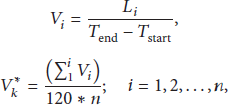
Average Velocity
3. Path Planning Algorithm
3.1. The Ant Colony Optimization Algorithm
Based on the path planning problem in intelligent transportation and the similarity of ant colony foraging and pathfinding, we can use the ant colony optimization algorithm to implement the path planning in intelligent transportation [13]. As in the whole system, different vehicles have different destinations; however, it is assumed that the vehicles share the same route as the same group of ants in the same road segment. When vehicles pass through a road segment, they transmit integrated traffic data to the information node, which are similar to the pheromones of the ant colony optimization algorithm. When subsequent vehicles plan a path, they can use these data as an important reference.
The parameters of ant colony optimization algorithm are defined as shown in the following.
The Description of Parameters
m: the number of ants (vehicles), α: determining the relative influence of the pheromone trail, β: determining the relative influence, ρ: Pheromone evaporation rate, Q: the intensity coefficients of pheromone which are increased,
Suppose there are m ants (vehicles) in the system, every ant has the following characters:
To select the next intersection according to the probability function with the value of the pheromones between intersections (suppose To ensure walking along the legal path, the ants being forbidden to access roads which they have passed before except when there is no other route to the destination which is controlled by the tabu table (suppose To update pheromones on every edge which it has walked along when the journey is completed.
At beginning, the initial value of pheromone on every path is unequal. Suppose


3.2. The Pheromone Computation of MACO
The key part of MACO is to determine parameter
Every intersection has some attribute values and every attribute needs a different weight. This shows the important grade, to calculate the pheromones in ant colony optimization algorithm. So set a weight value for each attribute of each outdegree of intersection as
3.2.1. Normalized Road Decision Matrix
Suppose each intersection contains m outdegrees; each of outdegree contains n attribute value in the road network; then the matrix below is formed:

3.2.2. Calculating the Weight Vectors
Let


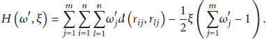
The partial derivatives of formula (10) are computed as

From formula (11), get

Normalizing the final weight from

So we have the weights of different attributes, and then we can obtain the data of every intersection.
3.2.3. Calculating the Positive and Negative Ideal Solutions
According to the weight value determined from (13), we can formulate the normalized decision matrix and obtain the positive and the negative ideal solutions as follows:

subject to
3.2.4. Calculating the Pheromone Values of MACO
Euler distance can be achieved with m degrees on each intersection node as follows:

According to the definition of TOPSIS method, the nearer it is to the positive ideal solution the farther it is from the negative one, the better the solution will be obtained. The pheromones of each outdegree can be achieved as follows:

Combining the experiment with the above algorithm, several other parameters in the ant colony optimization algorithm are determined as follows:

3.3. The Algorithm Complexity of MACO
The algorithm complexity of MACO is similar to ACO according to MACO based on ACO. We assume that m ants have to traverse n elements (intersections in this paper) after N circulations to get a solution of MACO. The effects of low power can be neglected if n is lager enough when calculating the time complexity, and the time complexity of MACO is
4. Simulation
We mainly pay attention to several different types in the process of navigation algorithm: time priority, distance priority, road condition priority, and integrated priority. Time priority refers to arriving at the destination with minimum time, distance priority refers to arriving at the destination with the shortest path, road condition priority refers to arriving at the destination with the best intersection line, and integrated priority preference refers to combining different road properties and then arriving at the destination with the least cost.
To illustrate conveniently, a road map measured with 8 by 8 squares is adopted to simulate road navigation. In the designed grid map (Figure 2), each intersection represents a road traffic intersection. Each node can adjoin the adjacent nodes bidirectionally. To stimulate path planning under different conditions, it is assumed that the path (49-56) and path (2-58) have two-way four-lane widths and other roads are of two-way two-lane width; here

The navigation path planning under different conditions.
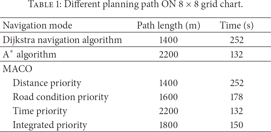
In the following, different navigation algorithms of MACO and two famous algorithms (the Dijkstra algorithm and the
Different planning path ON 8 × 8 grid chart.
Now we simulate with Zhuhai City map; as shown in Figure 3, we choose the area with 60 road intersections as coordinates. For each section between two adjacent intersections, we stimulate the path length, road width, road grade, and average velocity and then simulate MACO in SUMO environment and then carry on the simulation under velocity and time preference.

Normal traffic map in Zhuhai City.
As shown in Figure 3, the Dijkstra algorithm,
Statistics of three algorithms in normal situation.
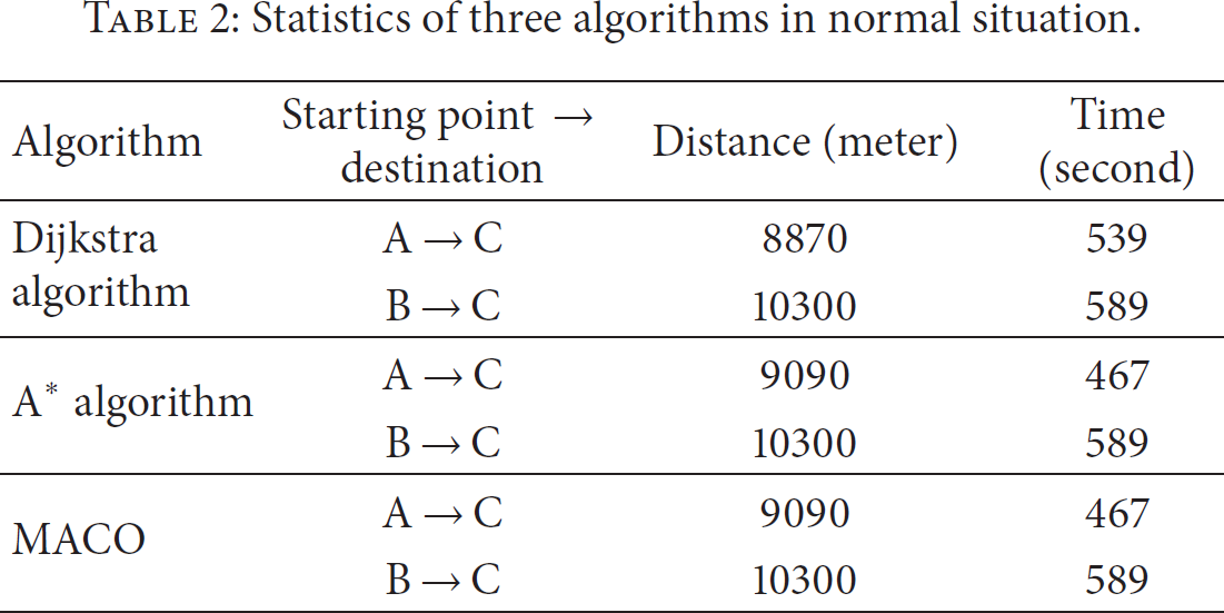
MACO can consider the comprehensive factors, so, from point A to point C, although the path planned by MACO is longer than the path planned by the Dijkstra algorithm, it still saves time since the average velocity is higher, which is the same as the
Among the above, the left convergence curves of Figure 4 are based on time (velocity) priority; the right convergence curves of Figure 4 are based on distance priority. On the left of the Figure 4 there are two convergence curves and we get the below convergence curve of travel time when we try to get a planning path only considering the high velocity or short travel time with MACO, and at same time we get the convergence curve of travel distance accordingly as the above one. And on the right of Figure 4 there are two convergence curves, too. We get the above convergence curve of travel distance when we try to get a planning path only considering the shortest travel distance with MACO, and at the same time we get the convergence curve of travel time accordingly as the below one. We can see that all the curves can be converged normally under two situations.

Convergence curves of MACO.
In order to further illustrate the advantages of MACO, simulation is carried out with this map and path, but set limited velocity in some sections as shown in the shadow part of Figure 5. Assuming that it is facing congestion, the simulation results are shown in Table 3.
Statistics of three algorithms in congestion situation.


Traffic map of congestion situation in Zhuhai.
From Table 3 we can see that if we set the shadow part as a traffic jam, the Dijkstra algorithm would not consider special cases and the path planned is still consistent with the normal circumstances, path length from point A to point C and point B to point C is 8870 meters and 10300 meters, but the time it takes increases to 803 and 872 seconds, respectively. And MACO fully considers the congestion; the paths planned are longer than normal and the path planned by the Dijkstra algorithm increased to 10380 meters and 11290 meters from point A to point C and point B to point C, but the time is less than the Dijkstra obviously, as 591 seconds and 663 seconds, which are consistent with the
MACO not only considers the integrated traffic information according to the requirement of path planning, but also can make path plans according to users' requirements. Below we still use Figure 5 traffic map and make analysis with only focusing on the path length, road width, average velocity, and comprehensive situation separately, as shown in Table 4.
Statistics under congestion situation using MACO.

According to Table 4, taking congestion into consideration, from point A to point C, the distance priority takes the distance of 8870 meters but the longest time of 803 seconds; the road condition priority only considers the road width which chooses the longest distance of 11600 meters and takes 655 seconds; it is similar between time priority and the integrated priority, the distance of 10380 meters, and takes 591 seconds. From point B to point C, the distance priority has the shortest distance of 10300 meters but takes the longest time of 872 seconds; the road condition priority planned the longest distance path for 12510 meters and takes 726 seconds in total; compared to the comprehensive case, time priority planned a longer distance path of 11530 meters and takes 647 seconds; integrated priority has a distance of 11290 meters and takes 663 seconds. From the above it can be concluded that the comprehensive situation, namely, integrated priority, takes account of path length, road width, road grade, and average velocity, so the distance and the time of the path planned cannot be the best, but it provides the optimal comprehensive solution.
The MACO has an important feature that it can plan path in real time with the dynamic traffic situation. Using ring map of Areia Preta in Macau, for example, these further illustrate the simulation results obtained by the algorithm as shown in Figure 6.

Map of Areia Preta in Macau.
Figure 6 shows two different situations in the urban traffic of Macau. The left of the maps shows normal traffic situation and that means there are no traffic jams. The right one of the maps shows the dynamic traffic situation, meaning that the traffic congestion is dynamically changing. The shadow part of Figure 6 is the traffic jam with an average speed of 20 km/h; other sections are normal traffic roads. Bold line shows two-way four-lane road with the average speed of 60 km/h and other roads indicate two-way two-lane roads with the average speed of 50 km/h. The unidirectional road segments are omitted for simplification. Simulation is carried out with the path planning from point A to point B. Also the Dijkstra algorithm,
Statistics of Macau under the real-time traffic situation.

The obvious differences are shown among three algorithms from the planned path. In the normal traffic situation, the Dijkstra algorithm plans a path whose travel distance is 1290 meters and the travel time is 104 seconds; it has the shortest path but the longest travel time. MACO chooses a path as good as the
In order to describe the algorithms in detail, suppose there are three cars travelling along the different paths planned above. When they travel to point C, the congestion happens in front of the path. Because they cannot plan dynamically the path according to the traffic situation, the cars adopt the planned path by the Dijkstra algorithm and the
From Figure 7, which shows the distance cost comparison of normal traffic situation and dynamic traffic situation, we can see that in two situations the Dijkstra algorithm and

The distance cost comparison of two situations.
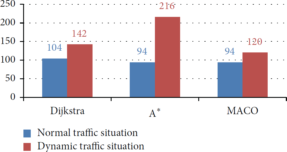
The time cost comparison of two situations.

The comprehensive cost comparison of two situations.
5. Conclusion
This paper has developed a novel multiple-metric ant colony optimal algorithm for vehicle path planning, in which four kinds of traffic attributes are considered, and some phases of the algorithm are discussed. A new general metric has been introduced as the pheromone value of ant colony optimization algorithm. Based on multiple traffic information and planning requirements, the proposed algorithm selects the most effective and suitable planning path. Simulation results demonstrate that the presented algorithm could easily achieve the suitable path according to different requirements, including the shortest path planning and the shortest time planning, in the real-time vehicular traffic networks. This algorithm provides a potential solution for energy consumption and environmental pollution in increasingly complex urban traffic environment, which could be used in intelligent transportation system.
Footnotes
Conflict of Interests
The authors declare that there is no conflict of interests regarding the publication of this paper.