Constrained Cross Entropy Localization Technique for Wireless Sensor Networks

Abstract

Challenges in wireless sensor networks (WSNs) localization are diverse. Addressing the challenges in cross entropy (CE) localization utilizing cross entropy optimization technique in turn minimizes the localization error with a reasonable processing cost and provides a balance between the algorithmic runtime and error. The drawback of such minimization commonly known as flip phenomenon introduces errors in the derived locations. Beyond CE, the whole class of localization techniques utilizing the same cost function suffers from the same phenomenon. This paper introduces constrained cross entropy (CCE), which enhances the localization accuracy by penalizing the identified sensor nodes affected by the aforementioned flip phenomenon in the neighborhood through neighbor sets. Simulation results comparing CCE with both simulated annealing- (SA-) based and original CE localization techniques demonstrate CCE's superiority in a consistent and reliable manner under various circumstances thereby justifing the proposed localization technique.

1. Introduction

The scope of wireless sensor network (WSN) applications is diverse. Regardless of the type of application, the sensed value is meaningful only if the location information is present. Protocols and applications such as routing and media access control often use location information especially in WSN perspective. Thus, localization is one of the most important issues for WSN deployments.

1.1. Background and Motivation

Having Global Positioning System (GPS) in every sensor node is not a practical solution for localization due to high device cost, power consumption, bulkiness, and poor accuracy (in specific locations such as indoors). Despite various research efforts for more than a decade, the localization problem remains an open research issue due to its challenges posed by large errors and high transmission and processing costs undesirable in WSN perspective.

Generally, for any localization algorithm, there must be a subset of nodes as anchors, whose exact locations are known a priori (through GPS or other means). Those algorithms take input of the distance and/or angle measurements between nonanchor and anchor nodes along with the anchors' locations and derive the desired location information of the nonanchor nodes. Depending on applications, localization algorithms calculate the relative or absolute positions of the nodes.

Primarily, there are four techniques to measure the distance between an anchor and a nonanchor node: receiving signal strength indicator (RSSI) [1], time of arrival (ToA) [2, 3], time difference of arrival (TDoA) [4, 5], and angle of arrival (AoA) [6]. RSSI utilizes propagation loss from transmit-receive signal strengths using theoretical or empirical propagation model and translates transmit-receive signal strengths into distance estimates. ToA/TDoA tracks propagation time of the signal (from transmitter to receiver) and translates the time measure directly into distance using signal propagation speed. Conversely, AoA technique measures the angle at which the signals arrived based on the delay of arrival at each receiver element which is then converted to AoA. Unfortunately, each of these measurement techniques has its own limitations. RSSI is cheap and available in common chip sets (built-in) but suffers from unreliability and randomness of the wireless medium especially due to the multipath propagation. TDoA provides good accuracy only if there exists a line-of-sight condition. Unfortunately random practical deployments do not guaranty such favorable condition. AoA can provide a reasonably accurate measurement with a high hardware cost as AoA hardware is practically an array of receivers. A higher accuracy requirement in angle measurement necessitates a higher number of receivers in the receiver array resulting in a higher hardware cost.

Generally, a localization algorithm employs one or multiple measuring technique(s) to get the measured distances between an anchor and its neighboring nonanchor nodes and then utilizes trilateration to infer the locations of those nonanchors. A number of localization algorithms [3, 7–27] have been proposed by different research groups. Most of those algorithms work well under their favorable circumstances. But still, none of them could always provide robust localization results under all possible circumstances in a consistent manner. Localization errors can be introduced under various challenging circumstances. Some examples include unfavorable node configurations such as poor positioning of anchor nodes, node geometry susceptible to flip and flex ambiguities [28], and real-world imperfections such as inherent distance measurement errors (of various measuring techniques as described above), limited transmission ranges of wireless sensor nodes, noises in signals, and obstacles in transmission paths. Once an error is introduced in estimating the location of a particular node X, this error becomes propagated to the estimations of the locations of other nodes which uses X in its triangulation. Again, such cascading errors occur in a random unpredictable fashion depending on the arbitrary sequence taken to process the nodes.

1.2. Our Contributions

Our objective is to overcome the challenges mentioned above and come up with wireless sensor node localization methods that perform robustly under various circumstances in a reliable manner. To achieve this objective, we propose constrained cross entropy (CCE) localization technique based on our previously developed cross entropy (CE) localization algorithm reported in [29]. The fundamental building block of the algorithm consists of the cross entropy optimization technique that minimizes the location estimation error based on the summation of the difference between estimated and measured distances among the neighborhood. The algorithm enjoys reasonably low processing cost compared to one of state-of-the-art algorithms, namely, simulated annealing (SA) [7, 19], while preserving almost similar error rate.

A common drawback of the multilateration techniques, including CE, that attempt to minimize the estimation error is commonly known as flip ambiguity [30–32]. In case some nodes in the neighborhood of the concerned node are located in such a way that they are approximately on the same line, then the estimated position may be in the flipped location with respect to the particular line. Our attempt to address the problem is devised by incorporating a constrained optimization technique where flipped nodes are penalized with a monotonically increasing weight. This technique is known as a penalty function method. Among the few candidates of the penalty function methods, we take the logarithmic barrier function method as our tool. With a higher processing cost, CCE exhibits a distinctive accuracy improvement compared to both SA and CE. In fact, processing power has a little impact as the algorithms are implemented in a centralized fashion where the target network is static rather than dynamic.

In summary, CCE, a localization application, provides a high level of accuracy for a static centralized network where the impact of processing power does not provide an important role. We have tested our proposed algorithm CCE, through simulation under a variety of circumstances, different percentages and configurations of anchors, different transmission ranges, and various noise factors, and have observed that the proposed CCE algorithm works well to meet the design objective in a consistent and predictable manner.

The rest of the paper is organized as follows. Section 2 presents a number of localization techniques available in the literature. The CCE localization technique is presented in Section 3. This section is concerned with the collection of measurements at the location server, the cost function for CCE, and the cross entropy optimization tool incorporated into the algorithm. Sections 4 and 5 present the simulation results and conclusions, respectively.

2. Related Works

A large number localization techniques have been developed by the research community [33, 34]. A class of localization techniques that are simple and lightweight generally suffers from high error in calculating location information. One of the simplest localization algorithms that estimates the centroid of the location of the anchor neighbors is introduced in [8]. Straightforward improvement of the algorithm adopts the weights for all neighbors and estimates weighted average for node location calculations [9, 10]. Incorporation of adaptive weights further improves the error performance in the system [11].

Another coarse-grain localization algorithm named DV-hop [12] roughly finds hop distances incorporating distance vector routing technique. A straightforward translation to actual distances on the nonanchor nodes in meter is then achieved by simple multiplication of the average hop lengths and their hop distance counts. RSSI-based DV-hop (RDV) improves the simple DV-hop performance by replacing the hop count to the RSSI based distance measurements [13].

Reference [14] first constructs a table of average RSSI versus discrete transmit power levels. The table is processed centrally to compensate the nonlinearity and thereby estimate the distances between nodes. Using sequential quadratic programming method the final results are achieved by minimizing the cost function.

In multidimensional scaling- (MDS-) based localization [15], the shortest distances of pairs are determined first (by Dijkstra's [35] or Floyd's [36] algorithm). The distances are then assigned as the elements of distance matrix of MDS. The classical MDS from the distance matrix provides a relative map of the nodes. An absolute map is derived incorporating the positions of the anchor nodes into the aforementioned relative map.

Nodes several hops away from the beacon enabled anchors deriving their locations by collaborative multilateration technique [37]. Nodes first approximate the region where it is located based on the beacon coordinates and then utilize Kalman filtering to update the positions. Nodes not directly connected to the beacons start with neighbors as a reference points where the nodes take estimated neighbor locations rather than real anchor locations. Using iterative calculations location information becomes refined throughout the network. It requires updating of location through transmissions. Though distributed, the transmission in each round is energy hungry and undesirable for WSN.

Reference [16] assumes nodes as point masses and the masses are connected through springs. Algorithm uses force directed relaxation method to converge to a minimum energy configuration. This heuristic graph embedding method uses a polar coordinate approach to the localization algorithm. Unfortunately the algorithm is vulnerable to be stuck into local minima.

Reference [17] initiates localization technique by outward broadcasting of hello messages (with duplicate suppression) from some specific nodes called seeds (nodes containing global location information). Upon receiving the broadcasts, nodes find minimum hop counts from the seeds. Upon finding such three different hop counts and seed location information nodes calculate their positions by finding the minimum of total squared error between calculated and estimated distances. The algorithm suffers from three distinct limitations: it requires high node density to keep the localization error reasonable; it incurs error if the hello message goes through a detour due to the obstacles; and it consumes undesirable amount of energy as using broadcasts.

Reference [18] uses minimum mean square error (MMSE) [38] algorithm to solve the location estimation of sensor node by minimizing the difference between measured and estimated distances. The algorithm requires a high density of node, alternately a high transmit range to make the estimation from a reasonably large neighborhood cluster [39, 40].

Simultaneous perturbation stochastic approximation (SPSA) based technique [20] minimizes the estimation error through a constrained optimization technique. SPSA attempts to correct geometric artifacts in localization by utilizing a penalty function; however it does not address the problem of flip ambiguity.

Simulated annealing- (SA-) based localization [7, 19] solves the minimization problem with simulated annealing technique. SA provides a reasonable error performance but suffers from poor algorithmic runtime efficiency. However, the algorithm is evaluated with at least three anchors in the neighborhood for all nonanchor nodes, which is deemed an impractical deployment for the randomly deployed sensor networks. In [29] we present CE based localization technique providing similar error efficiency with an improvement of algorithmic runtime. Unfortunately the algorithmic runtime in such centralized architecture with a static network undermines the importance of such algorithm.

The algorithms SA and CE suffer from a phenomenon called flip ambiguity [30–32] which is addressed by our modified cost construction in CCE. In our experiments, we employ SA and CE as benchmarks to evaluate and justify the relative performances of our proposed CCE algorithm.

3. Constrained Cross Entropy (CCE) Algorithm for Localization

Let N be the total number of nodes deployed in the network, and A is the number of anchors among them. The localization problem is therefore involved in finding the $[x,y]$ coordinates of $(N-A)$ number of nonanchor nodes. The fundamental idea of CCE localization algorithm is using the well-known cross entropy optimization algorithm to minimize the cost function of corresponding algorithm. Refer to [29] where the CE localization estimates the location based on the measured distances of the nodes from its neighborhood. CCE retains the basic principles of CE with a modified cost function to perform a constrained optimization by incorporating a penalty approach. The underlying idea of CCE design is to address one weakness of CE commonly known as flip of node locations [30–32]. Figure 1 shows the functional block diagram, that is, the detailed algorithmic steps in the proposed CCE localization algorithm.

Figure 1

Functional block diagram of CCE algorithm.

3.1. Obtaining Distance Measurements

First, we must acquire the distance measurements of the individual nodes corresponding to its neighbors for all nodes N. Second we must obtain A number of location information, that is, $[x,y]$ coordinates of the anchors. These two sets of information are the primary inputs of the localization algorithms including CCE. Protocol initialization involves collection of the aforementioned inputs at the centralized “location server” engaged by the following four steps.

• (i)

Create neighbor lists by localized hello messages without rebroadcasting.

(ii)

Measure neighbor distances by transmit-receive signal strengths/times from the aforementioned hellos (we can use any of RSSI, ToA, and ToDA methods or any combination of them for that purpose).

(iii)

Update location server with all distance information.

(iv)

Update location server with all anchor coordinates.

The localization server receives the data and uses constrained cross entropy-based localization algorithm (CCE) and derives the unknown locations for the nonanchor nodes. Generally designing protocols and algorithms in WSNs adopts distributed approach. But implementing localization algorithm optimization technique for CCE in a distributed fashion is not a suitable option. Optimization techniques update states in iterations and in each update algorithm needs the information of the states of its neighbors. In case of a distributed implementation the updates need explicit information exchange using active messaging and thereby would be costly in terms of energy consumption. Centralized implementation approach only requires sending the data to the central point once which is rather comparatively more efficient compared to the distributed approach.

Before going into the cross entropy optimization algorithm in detail, let us define the cost function relation to CCE.

3.2. Cost Function

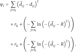
As stated earlier, unreliable nature of wireless medium introduces errors in capturing distance measurements. Localization techniques commonly estimate the locations of the nodes by minimizing the estimation errors [7, 18, 29]. We take such cost as the fundamental building block of the localization technique. Let $[{\widehat{x}}_i,{\widehat{y}}_i]$ and $[{\widehat{x}}_j,{\widehat{y}}_j]$ be the estimated coordinates of the nodes i and j. The estimated distance ${\widehat{d}}_{ij}$ between them can be simply calculated as ${\widehat{d}}_{ij}=\sqrt{({\widehat{x}}_i-{\widehat{x}}_j)+({\widehat{y}}_i-{\widehat{y}}_j)}$ . Let $d_{ij}$ be the measured distance between nodes i and j. Now, the cost function becomes

$$\begin{array}{cc}& {\psi }_i={\displaystyle \sum }_{j\in n_i}‍{\left({\widehat{d}}_{ij}-d_{ij}\right)}^{\mathrm{2}},\end{array}$$

(1)

where $n_i$ is the set of all neighboring nodes of node i. The goal of the optimization technique in CE/SA is to minimize the aforementioned cost while deriving the desired $[x,y]$ coordinates for the nonanchor nodes. With the measured distances and the aforementioned cost function, the aforementioned algorithms solve the localization problem in an iterative learning manner.

The said cost function attempts to minimize the sum of the distance errors unfortunately susceptible to some relative neighbor arrangements. More specifically if a subset of neighbors forms a straight line the derived node location may flip to the opposite side of the straight line commonly known as flip ambiguity [30–32]. The phenomenon is common to all localization techniques which adopt this specific cost function. In extreme cases the whole neighborhood can be in the flipped location. Such undesirable flips create large errors in localization. Non-coarse-grain localization techniques must take necessary measures addressing the flip ambiguity. Identifying and handling flip ambiguity to a degree is possible by evaluating the incorrect neighbors.

In case an estimated location of a specific node reviles a missing neighbor from the neighborhood list (derived from hello messaging) a penalty is added to the original cost. Similarly identifying an additional node in the neighborhood comparison which is originally absent should also be penalized. The incorporation of these penalties makes the optimization problem a constrained optimization problem. We define the cost function with constraints for CCE:

$$\begin{array}{l}{\psi }_i=\sum _{j\epsilon n_i}{({\widehat{d}}_{ij}-d_{ij})}^2\text{s}.\text{t}.\hfill \\ \hspace{0.17em}\hspace{0.17em}\hspace{0.17em}\hspace{0.17em}\hspace{0.17em}\hspace{0.17em}{\widehat{d}}_{ip}\le R\hspace{0.17em}\hspace{0.17em}\hspace{0.17em}\hspace{0.17em}\forall p\hspace{0.17em}\hspace{0.17em}\epsilon \hspace{0.17em}\hspace{0.17em}{n}_i,\hfill \\ \hspace{0.17em}\hspace{0.17em}\hspace{0.17em}\hspace{0.17em}\hspace{0.17em}\hspace{0.17em}{\widehat{d}}_{ip}>R\hspace{0.17em}\hspace{0.17em}\hspace{0.17em}\hspace{0.17em}\forall q\hspace{0.17em}\hspace{0.17em}\epsilon \hspace{0.17em}\hspace{0.17em}{\overline{n}}_i,\hfill \end{array}$$

(2)

where $n_i$ , ${\stackrel{-}{n}}_i$ , and R denote the set of neighbor nodes, the set of nonneighbor nodes of node i, and the radio range, respectively. Note that R is taken as uniform throughout the network to keep the problem demonstration simple. A variable R representing an individual radio range for each node can be adopted in a straightforward fashion.

The penalty function method changes the cost function of a constrained optimization problem in such a way that with the new cost function the optimization problem becomes a general form of optimization without any constraints. Augmented Lagrange method, penalty function method, and quadratic programming are the common forms of penalty functions. Sequential and exact penalty transformations are the two different types of penalty methods. Among them exterior-point penalty method and barrier function method are the forms of sequential methods. The barrier functions can be inverse or logarithmic. To preserve the feasibility at all times we implement the logarithmic version of barrier function method in our localization technique. Consequently the modified cost function can be expressed as follows:

$$\begin{array}{l}{\psi }_i={\displaystyle \sum }_{j\in n_i}‍{\left({\widehat{d}}_{ij}-d_{ij}\right)}^{\mathrm{2}}\\ \hspace{1em}+r_k\mathrm{\ast }\left(-{\displaystyle \sum }_{j\in n_i}‍\ln \left(-{\left({\widehat{d}}_{ij}-R\right)}^{\mathrm{2}}\right)\right)\\ \hspace{1em}+r_k\mathrm{\ast }\left(-{\displaystyle \sum }_{j\in {\stackrel{-}{n}}_i}‍\ln \left(-{\left({\widehat{d}}_{ij}-R\right)}^{\mathrm{2}}\right)\right).\end{array}$$

(3)

Note that the derived cost function needs to be optimized with a suitable optimization technique (cross entropy optimization in our case). We now can treat the problem as a simple optimization problem and no longer as a constrained optimization. Here, $r_k$ is the monotonically increasing penalty function based on rounds.

3.3. Optimization Algorithm

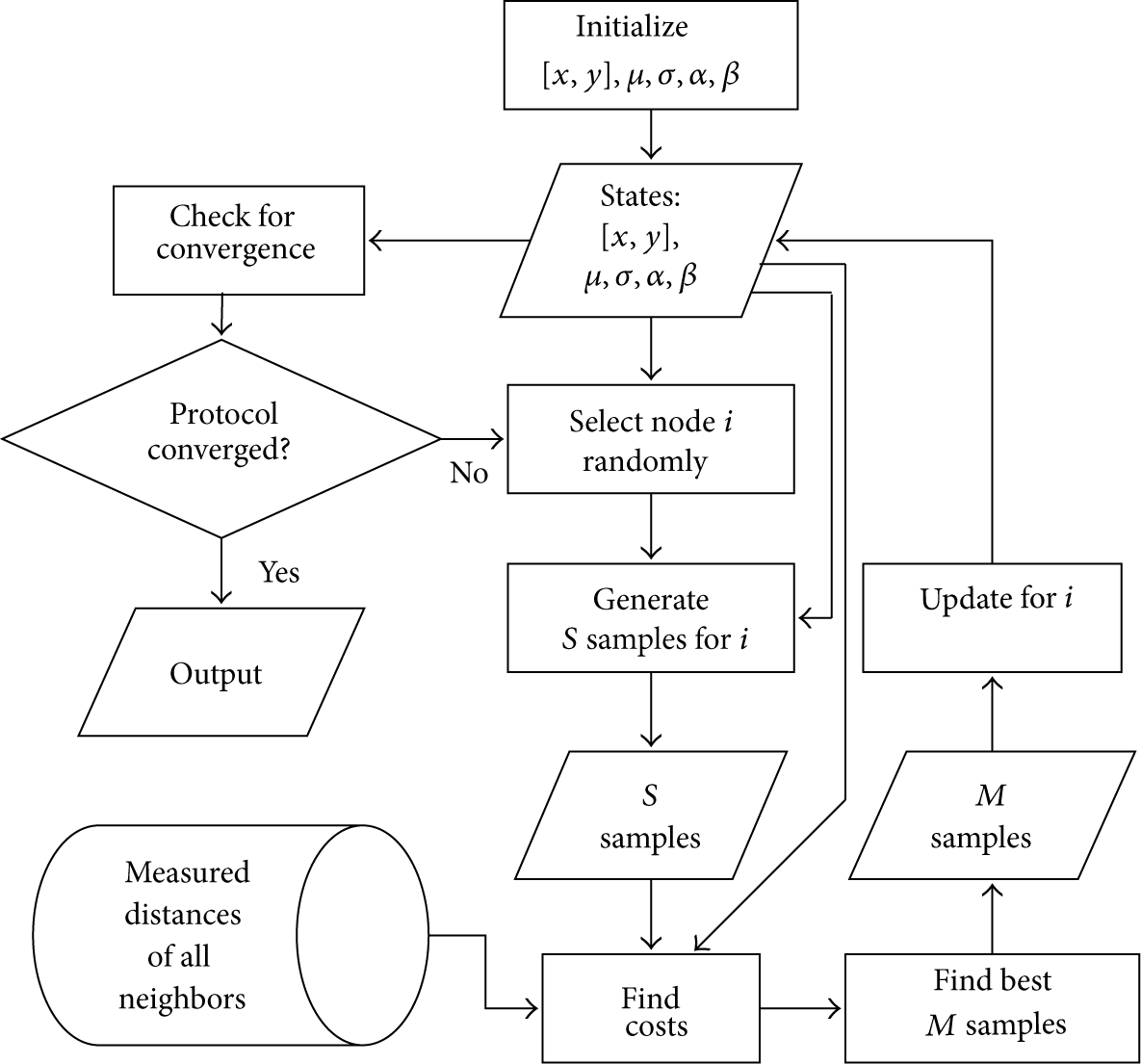
The proposed CCE localization problem derived from CE attempts to find the best coordinates of the unknown locations of nonanchor sensor nodes utilizing the cross entropy-based minimization of the aforementioned constrained cost. CE optimization technique is a method that attempts to integrate well-known techniques (1) combinatorial optimization, (2) Monte-Carlo simulation, and (3) machine learning and tries to exploit the advantages of them, all in a go [41] and thereby becomes our algorithm of selection in solving the localization problem for WSNs.

CE optimization algorithm generates samples based on the means and variances. Algorithm then selects the best samples as next state while it learns about the next generation samples' means and variances based on the best set of samples in the population.

In its first step, cross entropy optimization technique generates random states for all nodes. The algorithm then generates a set of populations for each state based on the mean and variance of that particular state. The algorithm then finds the cost for all the population based on the corresponding cost function. New generation of population is only selected in case the minimum cost of the population set is less than the cost function of the current state. In such case the state is updated; otherwise a new set of population is generated. In each state update the algorithm learns about better sample generation characteristics, where the characteristics are defined as means and variances and define the next generation samples. In an instance of an updated state, the mean and variance of that state are also updated based on the best population set. The algorithm updates the states iteratively until the cost or error is within the acceptable limit.

3.3.1. Initialization

On behalf of each unknown node $n_i$ the optimization algorithm generates the coordinates $[x_i,y_i]$ randomly and commonly known as state of the node. Here $n_i$ is a set of all nonanchor nodes denoted by $n_{\mathrm{1}}:n_{N-A}$ . Besides the algorithm initializes means ${\mu }_i$ and variances ${\sigma }_i$ for all $x_i$ and $y_i$ . Largely the initial means are set of random numbers and initial variances are set of ones, respectively, with a length of $(N-A)$ also used for our implementations. Alternately $\text{Ran}{\text{d}}_{\mathrm{1}}:\text{Ran}{\text{d}}_{N-A}$ and $\text{One}{\text{s}}_{\mathrm{1}}:\text{One}{\text{s}}_{N-A}$ are used as ${\mu }_i$ and ${\sigma }_i$ , respectively. The cost of all initialized states of the nodes is determined and subsequently known as initial best ${\psi }_i$ .

3.3.2. Iterations

The algorithm enters into an iterative mode after the initialization process. Iterations update the states until the desired refinement is achieved. The refinement is generally defined by several control parameters. The most important control parameter in this optimization is known as variance minimum. Another important control parameter is the learning rate. Generally two different learning rates are used for the means and variances denoted as ${\mu }_i$ and ${\sigma }_i$ , respectively.

The iterative method starts with generating a population of S number of samples for all $x_i$ and $y_i$ based on the means and variances of corresponding $x_i$ and $y_i$ . The samples are than evaluated and rated by the cost of a particular sample. If the cost of the best sample is less than best ${\psi }_i$ then the best ${\psi }_i$ is replaced by the cost of the best sample. The state $[x_i,y_i]$ is subsequently updated with the best sample for the particular node.

Updated sample number M is a tuning parameter of the algorithm and has impact on both the performance and the accuracy of the optimization technique. Algorithm selects best M samples by $x\mu bes{t}_i=\text{mean}(xbes{t}_1:xbes{t}_M)$ and $x\sigma bes{t}_i=\text{stddev}(xbes{t}_1:xbes{t}_M)$ corresponds to the means and variances of the samples, respectively. The mean of the best samples is used to update the corresponding mean of $x_i$ by $x{\mu }_i=\alpha \mathrm{\ast }x{\mu }_i+(\mathrm{1}-\alpha )\mathrm{\ast }x\mu bes{t}_i$ for the next generation of samples. Similarly $x{\sigma }_i=\beta \mathrm{\ast }x\sigma bes{t}_i+(\mathrm{1}-\beta )\mathrm{\ast }x{\sigma }_i$ is used to update the variance of $x_i$ . $y{\mu }_i$ and $y{\sigma }_i$ are updated in a similar fashion.

Algorithm trains the means and variances that in turn are used in generating the next generation population of samples. The superior samples in successive generations help algorithm estimate the better states, that is, the location coordinates in successive iterations. Contrarily, if the cost of the best sample is less than the best ${\psi }_i$ then the population set is discarded. And another set of samples is generated. After enough successive iterations the final state of i becomes the estimated location of the particular sensor node. A functional detail of the CCE localization technique is presented in Algorithm 1. The same information is depicted in flow chart format in Figure 2.

Algorithm 1: Constrained cross entropy localization (CCE) algorithm.

Constrained Cross entropy-based localization algorithm

 N: Total nodes

 A: Anchor nodes

 μ: Means

 σ: Variances

 α: Learning rate for means

 β: Learning rate for variances

 γ: Variance minimum

Node level measurements for all node  i

 Create neighbor lists

 Measure neighbor distances

 Update location server with

    all distance information

    all anchor coordinates

Algorithm at central computer

 for all unknown node i

  Randomly initialize [ $$x_i$$ , $$y_i$$ ] coordinates

  Randomly initialize μ and σ for $$x_i$$ and $$y_i$$

  Find cost for [ $$x_i$$ , $$y_i$$ ] and assign to initial $$BestCos{t}_i$$ by

    $$\begin{array}{cc}{\psi }_i=& {\displaystyle \sum }_{j\in n_i}({\widehat{d}}_{ij}-d_{ij}{)}^{\mathrm{2}}\\ & +\hspace{0.17em}{r}_k\mathrm{*}\left(-{\displaystyle \sum }_{j\in n_i}\ln \left(-({\widehat{d}}_{ij}-R{)}^{\mathrm{2}}\right)\right)\\ & +\hspace{0.17em}{r}_k\mathrm{*}\left(-{\displaystyle \sum }_{j\in {\stackrel{-}{n}}_i}\ln \left(-({\widehat{d}}_{ij}-R{)}^{\mathrm{2}}\right)\right)\\ & \end{array}$$

 end

 while (max(σ) < γ)

   for all i

    Generate S samples for $$x_i$$ and $$y_i$$

    Find costs for corresponding samples

    if (min cost of the samples < $$BestCos{t}_i$$ )

     Update state [ $$x_i$$ , $$y_i$$ ] with the best sample

     Update $$BestCos{t}_i$$

     Update μ and σ

     Select M number of best population

      ( $$xbes{t}_1$$ , $$ybes{t}_1),\dots ,(xbes{t}_M$$ , $$ybes{t}_M$$ )

     Take $$\mu best$$ and $$\sigma best$$ of the selected bests

       $$x\mu bes{t}_i$$ = mean( $$xbes{t}_1$$  :  $$xbes{t}_M$$ )

       $$y\mu bes{t}_i$$ = mean( $$ybes{t}_1$$  :  $$ybes{t}_M$$ )

       $$x\sigma bes{t}_i$$ = stddev( $$xbes{t}_1$$  :  $$xbes{t}_M$$ )

       $$y\sigma bes{t}_i$$ = stddev( $$ybes{t}_1$$  :  $$ybes{t}_M$$ )

     Update μ and σ with α and β respectively

       $$x{\mu }_i=\alpha \mathrm{*}x{\mu }_i+(\mathrm{1}-\alpha )\mathrm{*}x\mu bes{t}_i$$

       $$y{\mu }_i=\alpha \mathrm{*}y{\mu }_i+(\mathrm{1}-\alpha )\mathrm{*}y\mu bes{t}_i$$

       $$x{\sigma }_i=\beta \mathrm{*}x\sigma bes{t}_i+(\mathrm{1}-\beta )\mathrm{*}x{\sigma }_i$$

       $$y{\sigma }_i=\beta \mathrm{*}y\sigma bes{t}_i+(\mathrm{1}-\beta )\mathrm{*}y{\sigma }_i$$

    end

   end

 end

Figure 2

Functional details of CCE algorithm.

4. Simulation Results

We use Matlab to simulate the constrained cross entropy-based localization algorithm. We simulate 100 nodes in the 100 m × 100 m sensor field where the nodes are assumed to have radios with uniform transmission range. Modeling the measurement error is governed by the equation as follows:

$$\begin{array}{cc}& d_{ij}^m=d_{ij}^t\mathrm{\ast }\left(\mathrm{1}+\frac{g\mathrm{\ast }\text{nf}}{\mathrm{100}}\right),\end{array}$$

(4)

where the true and measured distances are denoted as $d_{ij}^t$ and $d_{ij}^m$ , respectively. Gaussian disturbed random variables g hold mean 0.0 and variance 1.0. $\text{nf}$ is the noise factor that regulates the magnitude of error.

Note that the random node deployments and algorithmic random number generations have impact on both time and error performance of the proposed localization technique. We employ 10 measurements for each evaluation and average them to fairly handle the aforementioned randomness issue deriving final results.

Our CCE optimization technique has a number of control parameters. Tuning the parameters is vital acquiring reasonably worthy results. For example, CCE control parameter variance minimum γ needs to be small enough to estimate acceptable location information. On the other hand too small a value for the variance minimum makes the simulation slow without much estimation improvement. With a number of trials we set $\gamma =\mathrm{1}{\mathrm{0}}^{-\mathrm{13}}$ . Learning rates α and β are set to 0.7 and 0.9, respectively. Finally sample number S and best sample number M are taken as 100 and 50, respectively.

Unless otherwise stated the radio range R and the noise factor are taken as 20 m and 10%, respectively. For all random deployments 4 anchors are placed at the 4 corners of the field.

We present error in our error performance evaluation as average error in the field defined in [7, 19]

$$\begin{array}{cc}& \text{error}=\frac{\mathrm{1}}{N-A}\mathrm{\ast }{\displaystyle \sum }_{i=A+\mathrm{1}}^N‍\frac{{\left(x_i-{\widehat{x}}_i\right)}^{\mathrm{2}}+{\left(y_i-{\widehat{y}}_i\right)}^{\mathrm{2}}}{R^{\mathrm{2}}}.\end{array}$$

(5)

Here the absolute and estimated locations of the $i\text{th}$ node are denoted as $[x_i,y_i]$ and $[{\widehat{x}}_i,{\widehat{y}}_i]$ , respectively. And the total number of nodes and anchors in the network is denoted by N and A, respectively.

We simulate CCE in both grid and random deployments and compare with SA where nonanchors are always in random locations.

4.1. Grid Deployments

In grid deployments we have equally distributed grids of 9, 16, and 25 anchors depicted in Figure 3.

Figure 3

Layout of grid deployments (anchors: 9, 16, and 25).

Figure 4 presents the RMS error with transmitter set to different transmit ranges from 13–20 m. The three subfigures show different results for 9, 16, and 25 anchors, respectively. In each case the proposed CCE outperforms the error performance of SA for the corresponding setting. Evidently SA has much poorer performances in case when the transmit range is set to a lower value. Setting a lower transmit range means a less number of neighbor nodes contributing to deriving node locations. Even with a less number of neighbors CCE has chance to better estimate the location by employing the constrain optimization. The opportunity of evaluating and correcting for the flip is the contributing factor of such better performance.

Figure 4

RMS error versus transmit range in different grid deployments (nf = 10%). In all the cases CCE outperforms SA. For lower transmission ranges CCE performs a lot better compared to SA. This is due to the fact that in lower transmission ranges nodes have less number of neighbors to assist in deriving locations. On the other hand CCE has opportunity to correct the location with additional information resulting from constrained optimization.

Figure 5 presents the performance of the localization technique in grid deployment in terms of different nf. A clear superiority of CCE over SA is demonstrated. In case of 16 and 25 anchors the error is negligible. Even with 9-anchor deployment the algorithm performs quite decently compared with SA. The most important observation is the slope of the curve that represents the impact of the increasing noise in the distance measurement. Slopes of CCE are much smaller compared to the others. It demonstrates that the protocol is less susceptible to the noise, that is, CCE nullifies the adverse effect of the noise to a greater extent. This is due to the fact that large measurement errors incurred due to the high nf are tackled by the constrain form of optimization in CCE.

Figure 5

RMS error versus noise factor (Tx range = 20 m). Clear superiority of CCE is demonstrated. Larger nf cannot push the error much as CCE corrects the error through flip identifications and corrections.

CE is originally designed to make the basic optimization problem of localization lightweight and it is shown in [29] that the design provides a balance between the error performance and algorithmic complexity. However this literature focuses solely on the algorithmic error performance rather than the other criteria algorithmic runtime.

We compare the CCE with CE and justify the additional processing complexity of the constrained optimization in CCE. Though error in CE is similar to SA in case of high anchor node deployments the error performance in CE in case of less percentage of anchors is poorer compared to SA. As a result the gain on the error performance over CE by CCE is significant. Figure 6 presents the performance comparison of CE and CCE for the grid deployments in various measurement errors. The figure demonstrates clear improvement over CE by CCE.

Figure 6

RMS error versus measurement error comparison between CE and CCE (in grid anchor deployments). Large amount of error from CE is eliminated with modified cost in CCE.

4.2. Random Deployments

In case of random deployments four anchors are placed in the four corners of the sensor field and the rest of the anchors are in random locations.

Figure 8 shows the convergence of a node location of CCE in rounds with 50% of anchor deployment. The pattern is quite random and may vary depending on: (1) relative locations of the neighborhood, (2) neighbor location reliability and (3) pseudorandom number generator of the CCE algorithm. Therefore the trace merely represents the algorithm; rather it can be taken as a single instance of a convergence.

Figure 7 shows the performance of all the algorithms in successive rounds where the transmit range and anchors are set to 20 m and 20%, respectively. Generally the algorithms converge exponentially. Here, CE converges the fastest with the worst error performance. SA has a little improvement on error over CE with the worst convergence rate. With little more rounds than CE, CCE converges better than SA in terms of both error and rounds.

Figure 7

Algorithmic performance in rounds (random deployment (Tx range: 20 m, anchor: 20%)).

Figure 8

Example node locations in rounds in algorithm CCE (random deployment (anchor: 50%)).

Figure 9 presents the performance of the random anchor deployments with 5 to 50 percent of anchors with 5% increment where the transmit range varies from 13 to 20 m. Similar to grid, random deployments show that CCE outperforms SA in all the cases.

Figure 9

RMS error versus number of anchors (random anchor deployments).

Figure 10 depicts the comparison of CE and CCE in difference transmit ranges (13–20 m) with 5:5:50 anchor deployments. As expected the CCE outperforms CE in all cases. The performance representing the figure conforms with the performance in Figure 6.

Figure 10

RMS error versus transmit range (random anchor deployments).

To capture how individual run performs rather than averaging by RMS we present each sample of the algorithmic run. We sort the samples from the best performance to the worst for both CCE and SA present in Figure 11. With only a few exceptions CCE shows better performance compared to SA. While averaging CCE always provides better error performance.

Figure 11

Error samples in different percentage of anchors (Tx range = 15 m). CCE outperforms SA with only a few exceptions. In most cases, CCE's RMS error is lower than SA's.

The simulation attempts to find various aspects of deployments grid or random; different percentage of anchors; different settings in transmission ranges; and different wireless channel conditions with varying noise factors. In all the aspects the proposed CCE performs better compared to CE and SA demonstrating a superior algorithmic design tackling error in localization.

We intend to refer to three diverse aspects of error handling in this context. (i) Choosing of the algorithm is vital in handling the measurement error. SDP localization technique [42] is one of the well-known algorithms based on convex relaxations. SDP has potential to actually be implemented due to its efficiency (fast execution). Unfortunately, with stringent error performance requirements the SDP may not be a suitable candidate as performance of SDP is even worse than SA. This is due to the fact that SDP as core algorithm does not handle the error in input elegantly. SA is somewhat superior compared to SDP as it can handle the measurement error incompletely and still suffers from the ambiguity problem. The core CE method fundamentally can handle measurement error and has similar error performance compared to SA. (ii) The CCE method further refines the error by handling ambiguity and provides superior location information. (iii) Simple CE handles error with specific variance quite well. The problem domain of the RSSI can have specific variance, that is, the variance in the field in a specific time is fairly constant without multipath. In fact CE can handle a varied variance with a different implementation named multilevel CE [43]. By implementing multilevel CE in CCE the algorithm handles both line-of-sight and multipath error in conjunction with the aforementioned flip ambiguity.

5. Conclusion

The constrained cross entropy localization technique has been devised in the context of WSNs. Fundamentally the technique attempts to estimate locations of nonanchor sensor nodes based on anchor locations and neighborhood distance measurements in a centralized fashion. The erroneous measurements introduced by unreliable wireless communications are tackled by minimizing the error between the estimated and measured distances by utilizing cross entropy-based optimization technique with constraints. CCE attempts to improve the localization error by engaging in flip ambiguity phenomenon in common estimation error minimization techniques employed in several localization techniques (SA, CE, and others). Flip ambiguity phenomenon is tackled by incorporating penalty function methods where penalty is delivered on the identified flip nodes. CCE results demonstrate its superiority on SA and CE in localization error performance. A major problem in localization techniques with small number of anchors and small number of neighbors is error propagation. Addressing such issue based on both CE and CCE is our future research direction.