
Abstract
Localization is emerging as a fundamental component in wireless sensor network and is widely used in the field of environmental monitoring, national and military defense, transportation monitoring, and so on. Current localization methods, however, focus on how to improve accuracy without considering the robustness. Thus, the error will increase rapidly when nodes density and SNR (signal to noise ratio) have changed dramatically. This paper introduces CTLL, Cell-Based Transfer Learning Method for Localization in WSNs, a new way for localization which is robust to the variances of nodes density and SNR. The method combines samples transfer learning and SVR (Support Vector Regression) regression model to get a better performance of localization. Unlike past work, which considers that the nodes density and SNR are invariable, our design applies regional division and transfer learning to adapt to the variances of nodes density and SNR. We evaluate the performance of our method both on simulation and realistic deployment. The results show that our method increases accuracy and provides high robustness under a low cost.
1. Introduction
Localization is ubiquitous in our life, such as in river pollution monitoring and early warning, urban air quality monitoring, wildlife monitoring and protection, and so on [1–3]. Accuracy is important for applications [4–7]. Many researchers are looking forward to improve the accuracy of the localization [8–10]. For example, Stoleru et al. [10] exploited the spatiotemporal properties of well controlled events in the network (e.g., light), to obtain the locations of sensor nodes. However, when researchers focus on the accuracy of localization, they ignore the robustness to the variances of nodes density and SNR (signal to noise ratio). As a result, when the nodes density and SNR have changed dramatically, the accuracy will decline rapidly. Many applications will benefit from considering the robustness to the variances of nodes density and SNR. For example, sometimes we need to locate objects’ precise positions in low-SNR circumstances (such as in workshop that is full of roar of machines) and in intensive-nodes circumstances (such as traffic jam during the rush hours), where the changes of nodes density and SNR will influence the accuracy of nodes.
Robustness has received much attention [11]. The key global approaches [12, 13] (a pending node needs to communicate with all the other nodes in the network and collects its localization data) in this domain are based on received signal strength RSSI and obtain weighted Euclidean distance proximity through the measurement of RSSI [14]. Some researchers augment these methods by considering the robustness through designing protocols [15] and algorithms [16]. However, underlying those methods is an assumption that the nodes density and SNR are invariable, which is unlikely in most practical deployment. Nodes density and SNR always change under different circumstances of environment (e.g., traffic jam or blast) in most cases. Besides, because of collection and calculation of data in the whole network, the methods suffer from high energy consumption, high communication cost, and high computational cost, which existing mechanisms [17–19] suffer from. However, the high energy consumption is always a challenge in communication field.
Most of the proposed methods use RSSI values,
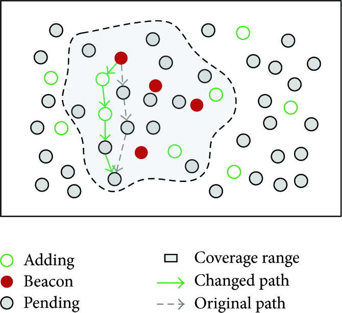
Examples for single-hop positioning problem and scale-weak problem. The red are beacon nodes and the grey are pending nodes. The range of beacon nodes just cover the nodes in grey area. When we use beacon nodes’ information to predict the location of pending nodes in grey area, the error is small while to predict the location of pending nodes outside the grey area, the error is big. That is single-hop positioning problem. And the shortest path from the beacon node to the pending node is the grey dash path. The green are the newly adding nodes. When adding these nodes, the shortest path from one beacon to a pending node changed from grey dash path to the green solid one. That is scale-weak problem.
This paper introduces CTLL, a Cell-Based Transfer Learning Localization method, which is robust to the variances of nodes density and SNR. In line with common practice in localization, CTLL employs beacon nodes, whose positions are known a prior. When the position of a pending node is queried, the pending node only needs to communicate with the beacon nodes that are in the same cell, which reduce the communication cost compared to global methods. Then we will obtain its position according to the trained model of each cell. The challenges however are how to design our cell-based beacon nodes, how to process the cell-based localization data, and how to train models for each cell.
Unlike past proposals, which have not considered the robustness to the variances of nodes density and SNR and the beacon nodes that are deployed randomly, we divide the whole network into many same size cells and then deploy the beacon nodes fixedly and uniformly in each cell. The pending node gets its position using the information that is obtained from the beacon nodes.
To illustrate CTLL's approach, Figure 1 shows a toy example, where the red nodes are beacon nodes and the grey nodes are pending nodes. As the figure shows, the range of beacon nodes just covers the nodes in the grey area in single-hop, when we use beacon nodes’ RSSI information to obtain the positions of the pending nodes that are outside of the grey area, the accuracy will be very low. When the topology of nodes changes, the shortest path from one beacon to a pending node changes from grey dash path to green solid path. Thus a robust localization scheme needs to consider the changes of nodes density and overcome the limit of single-hop problem.
So how can we locate the pending nodes in each cell? To do so, we need to employ SVR (Support Vector Regression) to achieve precise positioning. However, the difficulty of implementation is how to implement the SVR model on each cell. We use transfer learning to reduce the cost that comes form cell-based localization data. An important thing for SVR to implement localization is kernel function. Kernel function can map an inner product operation of high-dimensional space to the input vector function of low-dimensional space, and the mapping simplifies the computation.
In summary, the main contributions of this paper are as follows.
It presents a cell-based localization method that exploits regional division and beacon nodes are deployed fixedly and uniformly in each cell. As a result, the system is robust to nodes density and SNR. It also applies transfer learning and SVR to node localization and successfully uses them to implement node localization. It presents a low-cost solution for localization, no matter in communication cost, computational cost, or energy consumption.
The rest of this paper is organized as follows. In Section 2, the reason why we choose localization that is based on learning will be introduced. Section 3 is an overview of CTLL. This is followed by localization scheme design in Section 4. In Section 5, we show how we do localization in each cell. In Section 6, the implementation will be presented and experimental evaluations will be showed in Section 7. Section 8 will introduce the performance analysis. Then related work will be followed. Finally, conclusions are presented and suggestions are made for future work in Section 10.
2. Background
2.1. Connection for Localization between Geometry and Learning
For localization methods based on geometric features, the first step is to measure Euclidean distances between pending nodes and beacon nodes. After measurement, the algorithm can estimate the physical position of the pending node according to the measured dual distance between the pending node and a beacon node [20].
Current localization methods typically based on solving a multilateration problem:

A presentation of multilateration problem.
Generally, the dual distance d between a beacon node S and a pending node U can be calculated through the weighted shortest-path algorithm [21]. The path weights can be obtained from the signal propagation model:

According to maximum likelihood method, the nonlinear mapping relationship X can be calculated as
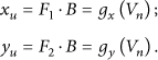
In (2),
2.2. Localization Based on Learning
Many learning-based methods have been proposed, as analysed above. The learning-based regression model [22, 23] has also been proposed. The regression model first measures the similarities among nodes. Then the regression model trains a learner based on the positions and the measured similarity of nodes. Finally, the positions of the unknown nodes will be obtained by employing the trained learner with the online measured localization data. Suppose that there are n nodes placed in a geographical region c. Let
(i) Signal Strength.
(ii) Weighted Shortest-Path Distance.
The objective for localization is to determine the positions of the remaining
The above step corresponds to the offline training localization model, and x-coordinate and y-coordinate need to be trained separately on a 2D space and produce two models. Then learned regression functions f which are based on
However, as shown in Figure 1, the red are beacon nodes which periodically transmit radio signals. The grey are pending nodes, which need to collect the localization data to estimate their positions. When using the localization data of the red nodes for SVR model training, the model just works well in the grey area. The nodes outside the grey area will get terrible results because red beacon nodes’ communication range just covers the grey area. If we expand the distribution region of the beacon nodes, the errors of both the grey area and outside grey area will increase. So, the contradiction between large distribution region of training localization data and generalization ability is prominent.
Besides, the movement or the access of nodes will also bring challenges. When there are new nodes joining in, which marked by green in Figure 1, the weighted shortest-path from the beacon to a pending node will change. As a result, the measured localization data appears to have large disturbance, and the disturbance needs the learned model to make some adjustments.
The challenges of model generalization and the change of nodes’ topology call for a careful consideration about the localization data themselves. We need a new way to manage the localization data which can trade off the training data distribution region and model generalization. That is to say we should reduce the negative effect of the movement or the access of nodes.
3. CTLL Overview
Different from the base stations used in GSM network, we use the beacon nodes (S nodes) to achieve the coverage of a cell, which is the basic unit in WSNs. Then, we use a local way to collect and handle the localization data in the cell. Each S node and non-S node within the region obtain their localization data just from each single cell. Based on those locally collected localization data, CTLL will establish learners to predict the positions of non-S nodes.
To locate a pending node at a high level, CTLL goes through the following steps, as shown in Figure 3.
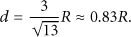
Divide the whole network into many cells with the same size. And the length of the cell is 0.83 R, which will be showed in Section 5. Deploy eight beacon nodes in each cell, and the number of beacon nodes in each cell will be demonstrated in Section 5. To locate a pending node, firstly we need to know which cell the pending node is in. All the beacon nodes in one cell send signals to the pending node. If the pending node can receive all the signals from all the beacon nodes which are in the same cell, we can make sure that the pending nodes is also in the cell. So the next work is how to locate the pending node in each cell? In each cell, we collect a certain amount of samples as the training set, and establish a regression model on the basis of the training set and SVR. Then the position of the pending node can be calculated when the localization data of the pending node is put to the model. Note that a pending node's localization is precisely the same to multiple nodes’ localization, because there is no need to collect localization data among pending nodes.

CTLL overview.
4. System Design for CTLL
This paper introduces CTLL, which solves the high costs and also improves the scalability and robustness of the system.
However, the efforts to use CTLL scheme for localization are based on two parts of work: the design and deployment of fixed facilities (S nodes) and the training of regression model in each cell. The design of the cell is the hard core of the scheme. And it includes the following aspects.
How many beacon nodes should we deploy in each cell? With the increase number of beacon nodes, the accuracy of localization improves while the communication cost increases accordingly. So we need to make a trade-off between performance and cost. How large should a cell be? If the cell is too small, we need to process many cell-based data, which will lead to the increase of computational cost; if the cell is too large, the pending nodes in the cell may not communicate with beacon nodes within the radio range. Why do we choose SVR regression model in the cell to locate the pending nodes? When we use SVR regression model, we need to use kernel function; what kind of kernel function can make SVR better and obtain minor error? When we use SVR regression model, we need to train a model in advance; thus we need to choose some sample points as the training set in advance. However, intensive sample points and sparse sample points in SVR model can achieve different results. So, how to choose sample points is also a question we need to consider. In order to locate the pending nodes in each cell, we need to collect sample points’ data in each cell, and collection work is huge and time-consuming. So instead of collecting data of each cell, how can we apply one cell's data to another cell? And that is transfer learning works.
4.1. Effective Number of Beacon Nodes in Each Cell
According to the requirement of geometry, there are two basic conditions needed to be satisfied when using multilateration for localization: (1) vector space mapping condition (physical quantity to be used for constructing the localization vector must be the function of dual distance, and the vector should involve more than three independent components); (2) position and number of beacons (beacons cannot be located in the same straight line; meanwhile, the number of beacons must be more than three).
RSSI is the function of dual distance, which can be used for constructing the localization vector. Meanwhile, beacons that exist in the network can be regarded as independent events to provide radio signals. Obviously, the RSSI vector will involve more than three independent components.
According to the derivation in [24], the Cramer Rao Lower Bound (CRLB) of the estimate position for one-hop multilateration can be calculated as follows:

In order to have a better understand of CRLB, Figure 4 gives four simple geometrical relationships between beacon nodes and the pending node in our cell. The distances between beacon nodes and pending node are equal in Figure 4. For example, there are three beacons, one is fixed and the other two move. The angles between the two moved beacons and one fixed beacon are separately α and β, which is from 0 to

Several simple localization scenarios for beacon nodes.
Now, from the perspective of entropy reduction, we analyze the differences among different numbers of beacon nodes used in the cell. When given the number of beacon nodes, the discriminative ability of beacon nodes for pending nodes in the cell can be calculated as follows:

In (4),
Dual distances between the pending node and beacon nodes are the same, because beacon nodes uniformly independently distribute around the pending node. And RSSI value v on

Equation (5) shows that the value of entropy reduction is negatively correlated with the number of beacon nodes N. Obviously, with more beacon nodes in the cell, it will have better discriminative power and gain more position information for localization.
In Figure 5, we define increasing rate as the ratio of the improvement of estimate error to the square of the increase number of beacon nodes, where the abscissa is the effective number of the beacon nodes, and the ordinate is the increasing rate. From Figure 5, we find that with the increasement of effective number of beacon nodes, the increasing rate decreases accordingly. When the effective number of beacon nodes is 7, 8, 9, and 10, the increasing rate changes very slowly. However, when pending nodes communicate with beacon nodes, the communication comes with certain cost. That means the more beacon nodes we deployed, the greater the communication cost is.

Relationship between the number of beacon nodes and the improvement of estimate error.
Based on the analysis above, in order to better deploy, we design our cell that consists of eight beacon nodes with a regular octagonal-shaped distribution.
4.2. The Size of the Cell
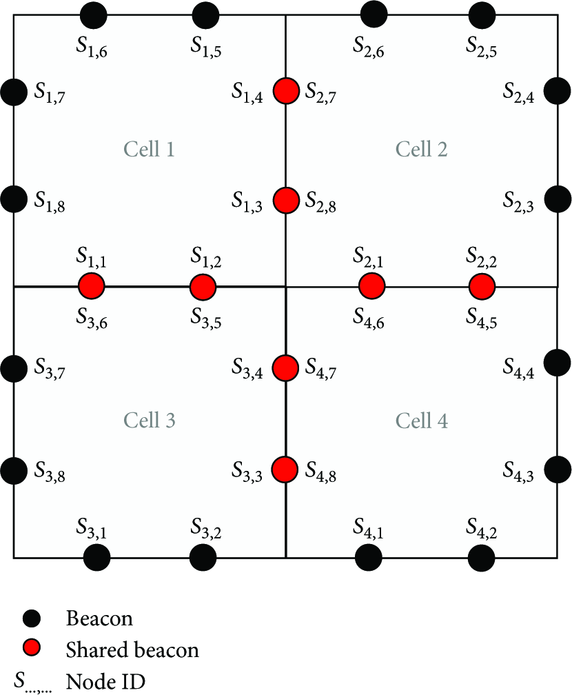
When we choose 8 as the effective number of the beacon nodes, the deployment of them is shown as Figure 6. Assume that R is communication radius of beacon nodes; eight S nodes scatter uniformly in the cell margin. Two adjacent beacon nodes evenly divide a side of a cell, and the length of each side is d (
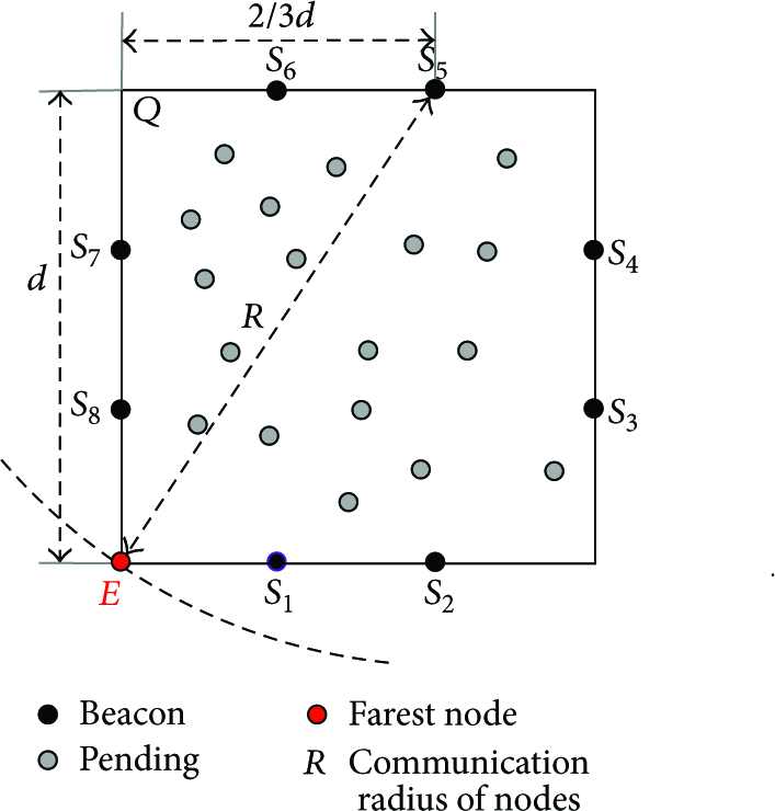
The basic structure of a cell.
Now, we discuss the cell side length d. As shown in Figure 6, eight S nodes are marked by black points, and every two adjacent S nodes divide a side length of a cell into uniform trisection. Because of the symmetry, we illustrate the relationship between R and d just on
Finally, our cell is a square area with side length d and eight octagonal distributed S nodes.
4.3. Why Choose SVR Regression Model
In the process of deployment, overfitting, underfitting, and local minimum are common problems; however, they can be better solved by using SVR [25].
SVR regression model develops on the basis of statistical learning theory, and the basic idea is that through kernel function, it can transform the training samples in low-dimensional inseparable input space into the feature vectors in high-dimensional liner separable space, thus avoiding the problems mentioned above.
For SVR regression model, we need to train a model according to training set so that when we input the test set, the model can predict the positions of pending nodes in the test set. The training set and test set consist of localization data of samples. However, we divide the network into many cells, so the model needs to have a good generalization performance so that we can use a small number of sample points to train the model. When we collect the data in data collection phase, the data collection needs to be proper and has a precise data set with noise.
SVR has a good generalization and ability to resist noise, using SVR regression model to locate pending nodes has the following characteristics.
In case of small number of sample points, SVR can achieve good generalization performance. SVR has good noise resistance; it can reduce the influence of measured noise on the results of localization and improve the positioning accuracy. Half a free style WSNs (beacon nodes deployed fixedly and pending nodes deployed randomly) has a good applicability, because it can respectively build SVR regression model according to different basic positioning cells.
The characteristics of SVR model just suit the requests of the model that we are looking for, so we choose SVR regression model in each cell to locate the pending nodes.
4.4. The Choice of Kernel Function
When SVR regression model is used to train a model, the choice of kernel function has big impacts on predicted positions, and these impacts are listed as follows.
From the perspective of space mapping, when we use kernel function instead of vector inner product for regression model, kernel function can determine the nonlinear transformation rules that is from low-dimensional input space to high-dimensional linear separable space. Thus if we change the rules by changing the expression or parameters of kernel function, the results of regression fitting and prediction results will change. From the perspective of sample similarity (there exists the inner relationship among the nodes located in different positions, and the inner relationship can be reflected through the sample similarity based on distance or the signal strength vector among nodes), the prediction results depend on the similarity between unknown samples and training samples. SVR measures the similarity between samples through inner product operation in high-dimensional linear separable space; thus the calculation of sample similarity and the prediction results will change if we change the type or parameters of kernel function.
Kernel function reduces the amount of calculation by transforming complex inner product of high-dimensional space into vector function of low-dimensional input space [26].
The type of kernel functions is usually chosen according to empirical knowledge, and the parameters are optimized by cross validation. For node localization in WSNs, the kernel function needs to have good prediction effect for the model, simple form, and a few parameters. Wu et al. [27] said that the RBF kernel function is commonly used as the kernel for regression. And Huang and Siew [28], Lin and Liu [29], Min and Lee [30], and many other also demonstrate the choice of RBF kernel function in their papers. In addition, in this paper, we compared the localization performance of SVR under three types of kernel functions: linear kernel function, polynomial kernel function, and the RBF kernel function. We do the experiment in simulation environment, different types of kernel function in SVM correspond to different values, and we just need to change the corresponding values in SVMtrain (train a model for SVR according to the input training set) when we want to change the types. The results are shown in Figure 7, and the mean error is calculated with 200 training samples and 200 test samples. From Figure 7, we can know that the error is the minimum when using RBF kernel function, meanwhile RBF kernel function contains only one parameter and has simpler form compared to linear kernel function and polynomial kernel function. According to the analysis above, we choose RBF kernel function for SVR regression model in this paper.

The relationship between localization error and type of kernel function. And the deviation is standard deviation that calculated with 200 training samples and 200 test samples.
4.5. How to Choose Sample Point
Distribution region of training samples is the learning region of SVR. If the more intensively training samples are distributed, the more fully SVR regression model is learned and the SVR regression model has higher generalization ability in the region. However, the intensive distribution of training samples will cause the increase of computational cost in regression model and model error.
Training samples are the basis of SVR regression model, and they correspond to the points in feature space (called the training sample points). The localization method of SVR model constructs input vector of training samples according to the coordinates of sample points in network area. Thus, the distribution of sample points affects the spatial distribution of training sample points.
When we choose sample points in sparse samples model, the distribution of sample points in feature space cannot be close to the pending nodes, so the regression fitting curve that is obtained by using sparse model is inaccurate. However, in intensive sample model, the distribution of sample points in feature space can extremely close to the pending nodes. So the regression fitting curve that is obtained by using intensive model is more accurate.
However, sparse distribution of the training samples will bring two problems: computational cost of regression model increases and model error increases. The similarity between adjacent training sample points is higher in intensive distribution. However, the resolution of SVR model for adjacent training sample points is very poor, thus causing the increase of model error.
The relationship between distribution of sample points and distribution of training sample points makes the choice of sample points’ distribution very important. The more intensive sample model, theoretically, makes the regression fitting curve more accurate. But we need to weigh the following two points.
Sample pattern should not aggravate the calculation in the regression model process. Sample pattern should not expand the model error.
4.6. Why Do We Need Transfer Learning
Because there are many cells in the whole network with the geographic variation, we need to collect data and construct SVR models for each cell. However, the labor cost is too high due to a large and repeated collection of data. To solve the problem, the transfer learning can provide a unified management of the training samples to separate them from their collection for each cell.
Transfer learning, as a method of expired data reuse, can obtain valuable information from the expired training data and thus transform and share information between different scenarios. Through transfer learning, the expired positioning scenarios of training samples still can be used to train in new positioning scenarios. Thus it greatly reduces the demand for the number of training sample points in positioning process. It makes the generalization performance of positioning model better in the area under the situation that the spatial distribution of sample points is invariable.
Being inspired, we propose SVR local regression model based on sample transfer learning, which deploys a supercell in advance and is dedicated to collect training samples. In actual deployment of a supercell in half a freestyle WSNs, the supercell can be applied to each local positioning unit cell by adjusting the weights of these collected training samples. By adjusting the weights, the SVR regression model is built with low cost. In this paper, we choose TrAdaBoost [31] as the transfer learning algorithm.
5. How We Do Localization in Each Cell
We use the cell as basic unit to train the localization data; it means that a pending node just needs to communicate with eight beacon nodes in a cell where the pending node is located. As each localization data on single cell is one-hop localization, we use SVR formulated in (7) to train the regression model and to predict the positions of pending nodes in cells.
SVR is to find an appropriate w, so that the regression loss is minimized. Localization problem under a soft-margin SVR framework is

Theoretically, if training localization data x and nodes’ positions y are infinite and measure noise on x does not exist, SVR regression model can accurately describe the mapping between x and y. However, only a small amount of localization data can be used for SVR model training, because the deployment of the nodes cannot be very intensive. Then it will cause the model effect error due to the estimation error with the approximate mapping relationship. Meanwhile, each cell needs to collect a priori data to train a regression model for itself, and the number of cells will decide how many times we need to do the collection work. The cost will be very expensive since there are many cells in the whole network. In order to deal with this problem, we employ a special cell called supercell and use the transfer learning approaches TrAdaBoost [31] to realize the data reuse from supercell to other cells.
A supercell is a predeployment test cell with intensively deployed nodes, which can be used to provide intensively distributed localization data and is represented by
Step 1.
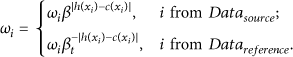
Set weight
Step 2.
Redo the following operation N times.
Set Get new learner h based on the weight distribution p on Get probability
Set

Step 3.
Based on weights of
The specific steps for localization in each cell are as follows, and this also shows how CTLL works. Assume that the network is connected and the pending nodes can communicate with the beacon nodes directly because the basic unit cell is small enough. And they use the signal strength information as the feature vectors to estimate the positions of pending nodes. There exists a basic routing protocol to provide the received signal strength The pending nodes communicate with 8 S nodes and record the information of packets such as the ID and signal strength and obtain an eight-dimensional signal strength vector Use the grid of size Normalize the input vectors and output coordinates for the training samples. And for the training samples set Construct the auxiliary training data set Choose the type and parameters of kernel function, and regularization parameter. Based on training samples X that is selected by TrAdaBoost [31], we can, respectively, construct the SVR regression model function The vector
6. Implementation
6.1. Prior Work
In this part, we will introduce the deployment of network, collection, and management of cell-based localization data.
Network deployment needs two steps to be completed: one for beacon nodes (S nodes) and one for pending nodes (non-S nodes). S nodes follow the octagonal deploy, and the entire network then will be divided into several cells with side length d, as shown in Figure 6. So, if network is
Symbol for S node.

True deployment of beacon nodes in large scale.
After deploying S nodes, we need to locate pending nodes. There are two steps for locating a node in the whole network. First, the pending nodes send signals to all the beacon nodes; if each beacon node in a cell can receive the signals, the pending node is thought in that cell. If the pending node falls on the junction of several regions, it will be calculated by the beacon nodes in several cells, and we can calculate their average as the pending nodes’ position.
Second, when we know the coordinates in the cell, how do we know the coordinates in the whole network? The actual coordinates in the whole network can be regarded as the coordinates in the cell add the relative coordinates. And the relative coordinates can be regarded as the number of the cells in front of the cells that pending nodes located in. And it can be calculated as the number of the cells multiply the side length of the cell.
When the deployed beacon nodes fail, the estimate position of the pending nodes may appear as errors. And then, the pending nodes need to send signals to all the beacon nodes in the cell to check which beacon node fails. If the pending nodes cannot receive the signal from a bacon node, we think the beacon node fails and then we change the beacon node.
6.2. Experiment Setup
6.2.1. Parameter Configuration
The real environment is located in a square of our campus, and we use the MICAZ nodes with chip CC2420 as sensor nodes and set the radio frequency 2.4 GHz. All the sensor nodes are put in the brackets which the height is 0.95 meter, as shown in Figure 9. In simulation experiments, we use (1) to produce RSSI information, and set the environment factor

The scenario of true deployment, square in the campus.
6.2.2. Experiment Scenario
In the real experiment, we use two days to deploy nodes. On the first day, we deploy supercell in the area of
7. Simulation Results
7.1. The Effect of Sample Points of Training Samples on SVR Model Error
In this section, the two parts will be considered: one is how many sample points we should choose, and the other is when we choose sample points, what is the interval between sample points?
Firstly, we consider how many sample points we choose as training samples is proper. To find a better number of sample points as training samples, we collect the information data from the random distribution of 18, 19, 20, and 48 nodes in the cell area and obtain the positioning errors of all the positions using SVR locating method. Figure 10 is experimental results, and it is the probability distribution of the predicting errors of all positions, and 88% of the position error is less than 1.5 m in four cases. It can be seen from Figure 10 that the predicting error is getting bigger with the increase of number of the sampling points in the region. The reason is that with the decrease number of sampling points, the differences of the RSSI signal vectors between nodes are getting greater, and the discrimination of different positions for SVR is getting higher. On the contrary, with the increase number of sample points, the deployment will be very intensive, the similarities of the RSSI signal vectors between nodes are very high, and the discrimination of different positions for SVR is very low, and that will lead to the increase of predicting errors. Therefore, the density of sampling points needs to be considered and chosen carefully in CTLL positioning method.
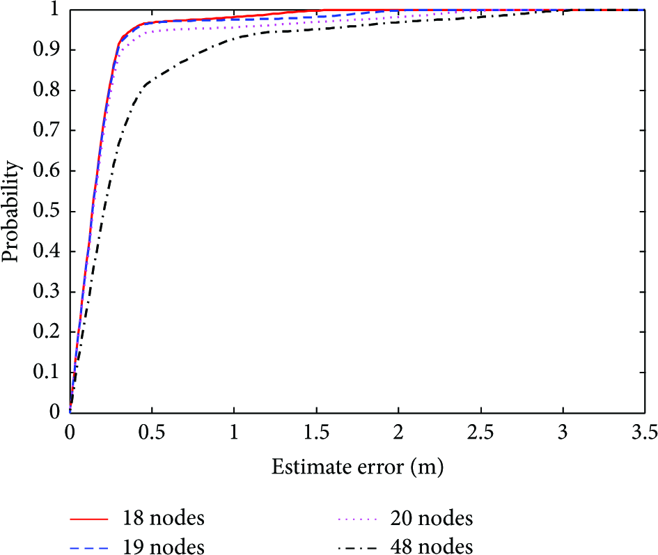
Relationship between sample points’ number and estimate error.
Secondly, when we choose sample points as training set to train a model, if the sample points are chosen very intensively in a small region, the model will cannot train fully in other region of the cell and we will get a big error. However, if the sample points are chosen very loosely in whole cell, the model cannot train fully in the whole cell. So how long is the interval between sample points appropriate? We collect the training set when the intervals between the sample points are 3 m, 4 m, and 5 m and get Figure 11. As shown in Figure 11, when the interval is 5 m, the model error is near 2 m in 73%, while the interval is 3 m and 4 m; the model error is near 1.5 m in 80%. When the interval is small enough, the model will train fully. However, small intervals between sample points aggravate the calculation of the model and communication costs between nodes. Thus we choose 4 m as the interval between sample points, and when the interval is 4 m, the model can get a better tradeoff between accuracy and costs.

Relationship between sample points’ interval and estimate error.
7.2. Parameters Chosen of SVR Model and Kernel Function
The parameters of SVR are chosen by cross validation [33]. Every 10 and 0.1 is adopted, and the search ranges are

The influence of SVR's parameters and RBF's parameter on estimate error.
The type of kernel function is usually chosen by empirical knowledge and the parameters of kernel function are optimized by cross validation [30]. For node localization in WSNs, the kernel function needs to have good prediction effect, simple form, and less parameters. RBF kernel function contains only one bandwidth parameter, simpler form, and good prediction results compared to linear and polynomial kernel function, thus becoming the first choice of kernel function.
Figure 12(c) shows how the parameter γ of RBF kernel function influence predicting mean error (
7.3. The Effect of the Number of S Nodes in Located Cell on the Result of CTLL Localization
In the previous phase, we have discussed the number of beacon nodes used in a cell based on reduction of entropy and CRLB. Considering the effect on errors, we take an experiment to see how the error changes when the number of beacon nodes increase. Because of even distribution of beacon nodes and the square cell, we conduct the experiment when the number of beacon nodes is 3, 4, 6, and 8. When the number of beacon nodes is 3, the coordinates are (0, 0), (30, 0), and (15, 30); when the number of beacon nodes is 4, the coordinates are (0, 0), (30, 0), (30, 30), and (0, 30); when the number of beacon nodes is 6, the coordinates are (10, 0), (20, 0), (30, 15), (20, 30), (10, 30), and (0, 15); when the number of beacon nodes is 8, the coordinates are (10, 0), (20, 0), (30, 10), (30, 20), (20, 30), (10, 30), (0, 20), and (0, 10).
Figure 13 shows the probability distribution of predicting error under different numbers of beacon nodes. The interval between sample points of predeployment supercell is 4 m. We predict 30 nodes’ positions that distribute randomly. We can see from Figure 13 that with the increase of beacon nodes’ number, the nodes’ predicting error is becoming smaller. When the number of beacon nodes increases from 3 to 8, predicting error reduces more than 4 m. And that shows the increase of beacon nodes’ number can help to improve the accuracy of CTLL localization.

The probability distribution of SVR positioning error under different numbers of nodes.
7.4. Sampling Density in the Sample Migration
In order to reduce the workload of collection, we deploy a supercell in advance and transfer supercell's information to given-cell using transfer learning. However, whether the interval between sample points in supercell influence the predicting error in given-cell is not sure. Thus we discuss the influence of node density in supercell on predicting error in given-cell, and then decide which node density will be chosen for our supercell predeployment.
The first step of CTLL algorithm is to deploy a supercell in advance, and the size of supercell is just as the size of given-cell. We set up sample points, collect the information of training samples in super-cell, and then adjust the weights of training samples by TrAdaBoost algorithm to make them meet the needs of each cell in actual deployment. As training samples, they can help establish a SVR regression model to predict the positions of pending nodes in each cell. Therefore, once the sampling area of supercell is determined, the sample density is just the factor that influences the performance of CTLL.
The definition of the sample interval: sample points are distributed uniformly in supercell area, and Euclidean distance between point and point becomes the sample interval. Therefore, the sample interval can be used as a measure of sample density. We will discuss the influence of the sample density on CTLL positioning error through simulation experiments. Set sample intervals of supercell 1.5 m, 2.5 m, 3.5 m, 4.5 m, 5.5 m, and 6.5 m, and we will predict 30 nodes’ positions that distributed randomly in given-cell. As shown in Figure 14, in accordance with the discussion results of actual deployment environment, with the increase of the sample interval, the error on the supercell decreases. However, on given-cell, with the increase of the sample interval, the error increases. Taking the error and computation complexity of CTLL into account, we will set the sample interval 4 m on supercell in simulation experiments.

Relationship between distance of sample points and SVR error.
8. Performance Analysis
8.1. Accuracy
We compared the performance of CTLL scheme with global methods under two types of global localization data: RSSI and weighted shortest-path. In order to obtain global localization data, a node needs to communicate with all other nodes in the network. In the first global method, we need to collect RSSI information between all the nodes to build eigenvector for localization. If the nodes cannot communicate with each other, the RSSI value is set to be −95, which is the minimum value that can be recorded. It is called RSSI-SVR. In the second global method, we need to collect weighted Euclidean distance between all the nodes to build eigenvector for localization. It is called proximity-SVR. The two methods obtain the nodes’ positions using SVR model. In simulation experiments, the global RSSI information is obtained using signal attenuation model, and proximity-SVR obtains weighted hop-counts distance using Floyd algorithm.
In actual deployment, we deploy 28 nodes and Figure 15 shows the predicting errors on a given-cell using three different methods: CTLL, RSSI, and proximity. The measurement and use of CTLL localization data follow CTLL scheme. It can be seen from Figure 15 that CTLL can obtain a better predicting error in most cases, except nodes 2, 4, 11, and 17.

Estimate error on different nodes in a cell for three methods.
Figure 16(a) shows the estimate error in a given-cell under different intensities of noise. We can see from Figure 16(a) that cell-based CTLL has the best capacity of resisting disturbance compared with the other two global methods. Not only the mean error of global method is bigger than CTLL, but also when the standard deviation of noise changes from 2 to 8, the mean error of global proximity method shows a larger fluctuation. Figure 16(b) shows the probability distribution of estimate error over the whole network, and it is measured when the standard deviation of noise is 2. We can also know from Figure 16(b) that the accuracy of CTLL is 95% when error is below 5 m, while the RSSI is 89% and proximity is 63%. Thus CTLL outperforms the two global methods.

Comparison between three methods.
8.2. Robustness
Robustness is a fundamental criterion in validating the scalability of the localization systems and it is also the superiority of our method compared with others. The movement and access of the nodes in CTLL just influence the number of pending nodes in the cells. We test the scale stability by changing the number of randomly deployed nodes in the given-cell. In Figure 17(a), when nodes’ number increases from 20 to 60, the differences between the probability of estimation errors are not obvious. Figure 17(b) shows that with the increase of noise intensity, the mean estimate error changes less obviously. It can be seen from Figure 17(b) that error distribution is similar under different noise intensities, except the maximum error. Thus, CTLL is not sensitive to the nodes’ number changing and noise interference. Those features make CTLL very suitable for localization in complex environment where the number of nodes usually changes and noise intensity changes.

Scalability of CTLL.
8.3. Communication Cost
Two main phases contribute to the computation of CTLL, and they are offline training phase and online localization phase. We collect pending nodes’ localization data in a supercell and beacon nodes’ localization data in each given-cell to train regression models. As the work of collection can be done in advance, we do not need to consider its communication cost. In our CTLL system, the communication only occurs in online localization phase. A pending node gets its localization data through single-hop broadcast to its neighbor beacon nodes. Assume that there are N nodes in the network; CTLL only needs broadcast N times to complete the positions prediction of N nodes. However, RSSI and proximity get their localization data by constructing the RSSI eigenvectors and weighted graph

Relationship between pending nodes and communication cost.
8.4. Time Complexity Analysis
The complexity of CTLL comes in two parts: the time spent on training a model (offline training phase) and the time spent on locating pending nodes according to the input model (online localization phase). Tsang et al. [34] pointed out that state-of-the-art SVM implementations typically have a training time complexity that scales between
Assume that there are A beacon nodes deployed and L pending nodes in the whole network, V is the number of supported vectors for SVR, and S is the number of training samples. SVM sees localization estimation as multiclass problem. And it uses the signal strength between pending nodes and A beacon nodes as input data; the output data is L positions, and each location use
We can know from the analysis above that the time complexity is associated positively with L pending nodes and S training samples. And then we run an experiment to see how the runtime changes when L and S change. For training set and test set, the number and positions of nodes are separately the same for CTLL and two global methods. In order to better understand the relationship among time complexity, the number of pending nodes and the number of training samples, we set the number of training samples in training set and the number of pending nodes in test set is the same. For example, when we have 100 nodes to locate, the training set also has 100 training samples. The runtime that locates those 100 nodes using CTLL is just a little bit more than 0.001 s (e.g., 0.0014 s) while locates those 100 nodes using global methods is a little less than 0.01 s (e.g., 0.0092 s). And the experiment is done using MATLAB R2012b on a 64-bit machine with Intel Core i3-4150 Quad-Core processor and 8 G memory.
8.5. Insensitive to Network Hollow
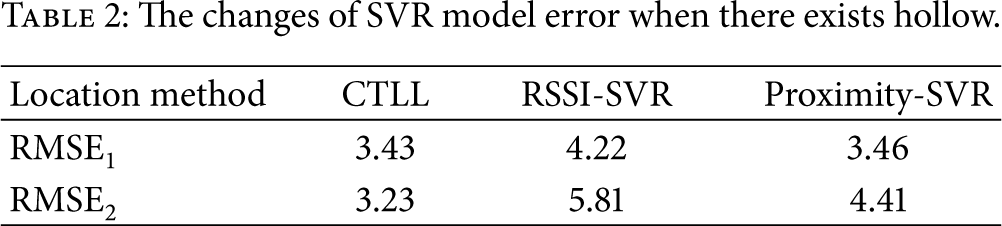
There is another superiority that CTLL has compared with global methods, and that is CTLL method is not sensitive to the network hollow. Figure 19 shows a network that contains the hollow. We deploy hundreds of nodes randomly in the network. Table 2 is the mean square error for three methods. RESE1 represents that there does not exist hollow in the network, while RESE2 represents there exist the hollow. We can see from Table 2 that the error increases 138% when there exists a hollow in the network for global RSSI method. Because the RSSI information comes from single-hop communication between nodes; however the collection of localization information on the edge of the hollow is not sufficient and the positioning results of edge nodes are more likely to fluctuate, and that will lead to the increase of error. We can also know that the error increases 127% when there exists a hollow in the network for global proximity method. Because the localization data of proximity need to be obtained through hop counts and when there exist hollow, the localization performance will decrease.
The changes of SVR model error when there exists hollow.

There exists hollow in the center of the network.
9. Related Work
Learning-based localization developed in the framework of statistical learning theory, and there are two types of learners: classification learner and regression learner. Since classification learner model relies on the discretely deployed region, we restrict our literatures’ review on the regression learner model.
Regression learner model based on the fact that nodes is deployed in a continuous manifold; the physical position can be used as a continuous feedback to build mapping relationship between localization data space and physical space. There are two types of localization data: global RSSI and global proximity. For the latter one, only proximity (or connectivity) information is available. The approach in [13] assumes that there exists a path between each pair of nodes, and the network is showed as an undirected graph
Recently, transfer learning [42] has emerged as a new learning framework to address the problem when we only have sufficient training data in one domain, and the other domain we interested is lacking of data to train an accuracy model for learning task. Pan et al. [43] assumed that a low-dimensional manifold was shared between two adjacent regional localization data and presented a transferring learning model approach that achieved the model building from one indoor area to another. Wenchen Zheng et al. [44] introduced a semisupervised Hidden Markov Model to transfer the localization models over time. In order to decrease the effects from complex environmental changes on the learned model, Zheng et al. [45] proposed a latent multitask learning algorithm to solve the multidevice indoor localization problem.
10. Conclusion and Future Work
This paper analyzes localization problem under regression model and its shortcomings on complex wireless network environment. According to CRLB and entropy reduction theory, we discuss and build CTLL scheme, which relies on the cells designed in the way like base stations in GSM. Localization data from single cells under CTLL scheme is complicated and wasted for nodes’ information collection, we use a predeployed supercell to simplify the localization data collection, then the instance transfer leaning TrAdaBoost method is applied to cells to establish accuracy regression models. We use many experiments to demonstrate the performances and find that CTLL scheme has better performance and stronger robustness over noise and scale when compared to the global methods.
We also believe that our CTLL systems will work better if the following factors are considered.
We only discuss simple positioning scenarios in the half freestyle WSNs in this paper. But in actual distribution, the network may need different cell models that are combined to be adapted to the environment. Therefore, the design of the basic units for positioning can be diversified; the network can contain different types and different sizes of the cell units, so that the network construction will be more in line with the needs of deployment of actual environment. We only consider the environmental differences in the sample migration in the design of the CTLL transfer learning in this paper and we do not take the differences of the equipment into account. There are multiple types of sensor devices in practical WSNs, and they come from different manufactures and have a different transmission power. Accordingly, in order to improve the popularization of CTLL method, we should also consider the differences of the sampling devices in sample migration. Due to the high labor costs of the deployment of network system, the network that we deployed is small and only contains 48 nodes. Large-scale network experiments get experimental data and results from the simulation environment because of the complexity of actual deployment in large-scale network. There will appear all sorts of unexpected problems in localization process, such as communication conflict and communication links randomization. As a result, we also need positioning analysis of large-scale actual deployment to increase the persuasion of the CTLL positioning method. Actual networks are mostly deployed in three-dimensional space; therefore, extensional algorithm is also needed to continue the study so that it can adapt with the demand changes that the localization changes from two-dimensional plane space to three-dimensional space; that will be the research direction in this paper.
Footnotes
Conflict of Interests
The authors declare that there is no conflict of interests regarding the publication of this paper.
Acknowledgments
This work was supported by the Project NSFC (61070176, 61170218, 61272461, 61373177, and 61202393), the Project National Key Technology R and D Program (2013BAK01B02, 2013BAK01B05), the Key Project of Chinese Ministry of Education 211181, International Cooperation Foundation of Shaanxi Province, China, 2013KW01-02, NSFC (61202198), China Postdoctoral Science Foundation (Grant no. 2012M521797), Northwest University School Support Foundation (14NW28), and International Cooperation Foundation of Shaanxi Province, China (2015KW-003).