Waypoint Graph Based Fast Pathfinding in Dynamic Environment

Abstract

Pathfinding is a fundamental task in many applications including robotics, computer games, and vehicle navigation. Waypoint graph is often used for pathfinding due to its advantage in specifying the space and obstacles in a region. Currently the waypoint graph based pathfinding suffers from large computation overhead and hence long latency in dynamic environment, where the location of obstacles may change. In this paper, we propose a fast approach for waypoint graph based pathfinding in such scenario. We eliminate unnecessary waypoints and edges to make the graph sparse. And then we design a prediction-based local method to handle the dynamic change in the environment. Extensive simulation has been done and the results show that the proposed approach outperforms existing approaches.

1. Introduction

Pathfinding is a fundamental task in many applications including robotics, computer games, and vehicle navigation [1–4]. Given a region that includes many obstacles and an object with a specific size, we need to find a proper path for the object from the origin to the destination. Waypoint graph [5] is widely used for pathfinding. Each node in such a graph is called a waypoint and specifies a special location in the region. An edge between two waypoints denotes that the object can safely go through it without collision with the region boundaries or obstacles. Based on waypoint graph, the pathfinding can be easily performed.

Compared with static environment, pathfinding in dynamic environment is more challenging, since the locations of obstacles may change from time to time. This is not uncommon in the real world. For example, in a subway that is on fire [6], the unsafe regions (i.e., the obstacles) change frequently and the rescuers need to revise their plans according to such information. For the waypoint graph based approach, when the locations of obstacles change, the structure of waypoint graph changes accordingly and makes the computation difficult. Pathfinding existing in dynamic environment needs a large amount of computation to reconstruct the waypoint graph and recompute the path based on updated graph. It incurs quite long latency. Considering that many applications including rescue tasks, vehicle networks, and online games need timely services, a fast pathfinding approach is highly demanded.

In this paper, we propose a fast pathfinding approach to address the aforementioned problem. We improve the waypoint graph model through two methods. First, we eliminate the unnecessary waypoints and edges that do not affect the computation result. Second, we segment the long edges to limit the length. This processing composes a sparse and localized graph and can greatly reduce the computation. After that we further adopt two methods to achieve fast pathfinding in the dynamic environment. First, we performed local update approach to revise the affected parts of the waypoint graph. Second, we predict the motion of moving obstacles to plan the paths for the objects. The prediction is quite important not only to speed up the pathfinding process, but also to be critical to achieve desirable performance in some emergency applications (e.g., fire rescue). We conducted extensive simulations to validate the effectiveness of the proposed algorithm. The results show that the proposed approach is effective and outperforms the existing approach. In summary, this paper makes the following contributions.

• (i)

We improved the waypoint graph model to reduce the computation overhead of pathfinding. It generates the sparse graph by eliminating unnecessary nodes and edges with bounded accuracy loss.

(ii)

We designed the fast approach for pathfinding. When the locations of obstacles change, only a few revisions are needed for pathfinding. Furthermore, pathfinding is based on the prediction of the motion of moving obstacles, which will further speed up, and enabling early alarm of dangerous situations.

(iii)

We conducted extensive simulations to validate the effectiveness of the proposed algorithm. The evaluation results show that the proposed algorithm is effective and outperforms the existing approaches in terms of the response time.

The rest of the paper is organized as follows: Section 2 reviews the related works. Section 3 formulates the problem in this paper. Section 4 describes our approach to build the waypoint graph. Then we describe how to locally handle the environment change in Section 5. After that, the path planning algorithms used in this paper are illustrated in Section 6. The simulation results for the proposed algorithm are reported in Section 7. Finally Section 8 concludes the paper.

This paper is based on our previous conference paper [7]. In this version, we extend the work to give more detailed waypoint graph model, propose the prediction-based handling of multiple moving obstacles, illustrate the local pathfinding algorithm, and also provide more analysis details and simulation results.

2. Related Works

The pathfinding has been investigated in many fields, especially in robotic navigation and artificial intelligence. It is quite difficult to find a proper path from the source to the destination in a free space. Therefore waypoint graph is usually used to facilitate the pathfinding process where the pathfinding is performed among special reference points called waypoints.

In Lozano-Perez and Wesle's visibility graph [8], the waypoints of a graph are defined by the vertices of obstacles, the origin, and the destination. A pair of visible vertices are connected by a straight line (called an edge). “Visible” means that there is no obstacle in the line between them. The path from the source to the destination is computed based on the reference points and edges. The path is collision-free which means that following it the object will not enter into any obstacle. This paper also considered the size of the object and the rotation of the object during the moving. The work [9] used a similar graph data structure for pathfinding problem. In later works, multiple objects are considered. The work [10, 11] computes the path for a crowd of objects successively. It means that a proper path is calculated for the first object and then this object is considered as a moving obstacle for the resting objects. This approach is easy to implement but suffers from large computation overhead and latency in the applications with a large number of objects. In work [12], a navigation graph is used to implement pathfinding in real-time and large-scale environment. The collision avoidance among objects is solved locally. The objects are intended to spread in different paths to mitigate the collisions. The work [5] proposed an automatic generation procedure of waypoint graph in 3D environment and supported the object's volumetric move which does not need to be strictly performed on surface. The work [13] investigates a new dynamic model to measure aesthetic values in pathfinding for videogames. In some works, the regions are divided into grid cells and the vertices of the cells are potential waypoints [14]. The work [15] proposed an autonomous-dynamic localization system which dynamically chooses establishing grids. In this kind of approach, the accuracy of the path depended on the size of grid cells. The works [16] investigate the difference between the shortest path based on grid and the real shortest path. The grid based algorithm is revised to achieve the real shortest path. These methods are designed based on the static environment, which cannot be directly used in dynamic environment due to their large computation overhead when updating the waypoint graph and lack of the motion prediction.

Instead of global path planning, some works investigated local pathfinding approaches. Khatib proposed the artificial potential field approach [17]. In that work, the object finds the path in real-time based on a field of forces. The position to be reached is an attractive pole for the object, and obstacles are repulsive surfaces for the objects. This model has to be widely used in many later works including [18]. The work [19] improved it by handling the inaccuracy of sensors that are used to detect the obstacles and enabling the continuous motion of objects without stopping in front of the obstacles. Vector field histogram approach [20] further overcomes the drawbacks of artificial potential field approach that the objects cannot enter narrow passages and have instable speed when traveling in narrow corridors. Rapidly exploring random trees (RRT) [21, 22] are developed to efficient robot navigation in a dynamic environment. The work [23] further improves RRT to obtain near optimal pathfinding solutions in short time. We think that the local approaches are suitable for real-time large-scale systems, so we follow this idea in the pathfinding.

3. The Problem

We formulate the problem discussed in the paper as follows. Given a region which includes several objects and obstacles, the region and the obstacles are denoted by polygons. The objects are denoted by a sphere with the radius of r (for the objects with other shapes, we can calculate its minimum bounding sphere (MBS) [5]). There are several exits in the regions. The obstacles can move or expand its occupied areas in the region. The motion/expanding of the obstacles can be predicted to some degree. Our objective is to plan the paths for all the objects such that they can reach the exits of the region in the shortest time without collision with any part of the moving obstacles. An application of the problem can be seen in Figure 1.

Figure 1

An example of pathfinding. It is a map of a shopping mall in the city of Wuhan, China. Black dots denote the persons. There are two fires (in red color) that expand their occupied areas constantly. And there are two dangerous objects (in blue color) that move in the region.

4. Waypoint Graph Generation

In our approach, we first generate the waypoint graph of the region and conduct pathfinding based on it. In this section, we illustrate the procedures of waypoint graph generation and our improvement for that. The goal of the improvement is to reduce the number of nodes and edges in the graph in order to reduce the computation cost.

4.1. Waypoint Candidate Generation

For each obstacle, we determine the waypoint candidates. Suppose that an obstacle is composed by a collection of edges. For each corner of the obstacle composing by two adjacent edges, a waypoint candidate is defined in the angular bisector of the corner, with a distance of r to the common vertex of the two edges. One example of that can be seen in Figure 2. We can prove that for each pair of adjacent corners the waypoint candidates of them, if not hindered by other obstacles, are reachable.

Figure 2

Waypoint candidates reside in the angular bisector of the corner and a distance of r to the vertex.

4.2. Waypoint Validation and Clustering

After the previous process, we get many waypoint candidates. We removed or clustered the waypoint candidates that do not affect the pathfinding computation. The left ones become the waypoints.

A waypoint candidate is regarded as a valid one if it is within the region boundary and is not hindered by obstacles. Otherwise, the waypoint candidate is invalid. The hindering condition means that other obstacles intersect with the circle of the waypoint (with the radius of r). Figure 3 shows an example of valid and invalid waypoint candidates in a region. All the invalid waypoint candidates are removed.

Figure 3

An example of valid and invalid waypoint candidates. The waypoint candidates are invalid if they are outside of the region (A, B, E, and F), inside the obstacles (H) or the circle centered with it is intersected by obstacles (G, I).

We further cluster the waypoints candidates. The region is divided into a $\mathrm{2}r\times \mathrm{2}r$ grid and the waypoint candidates belonging to the same grid are clustered. For each group, if its geometric center has no collision with obstacles, we use it as the new waypoint. Otherwise, we will randomly choose a location that is collision-free and near the geometric center as the new waypoint.

4.3. Complete Waypoint Graph Composing

After determining the waypoints, we now generate the edges and compose the waypoints graph. We first build a complete waypoint graph by connecting each pair of waypoints if the object can travel it without collision with obstacles. It is noted that since an object has a certain size, a sufficient large corridor is needed for them to go from one waypoint to another and in such corridor there should be no obstacles.

This procedure will generate a number of edges. Let $\left|W\right|$ be the number of the waypoints and let $\left|E\right|$ be the number of edges; in the worst case, there are $\left|E\right|=C_{\left|W\right|}^{\mathrm{2}}$ edges generated.

4.4. Incremental Graph Sparsification

In order to reduce the computation overhead, we build a sparse waypoint graph by removing some edges. Certainly making the waypoint graph sparse causes the accuracy loss of the pathfinding results. Therefore, we need to trade off the overhead and benefit brought with the sparse waypoint graph. In this paper, we revise the method proposed by Wardhana et al. [5] to achieve our goal.

In our solution, as shown in Figure 4, a square is used to help filter the edges of waypoints. Assuming that currently we want to filter the edges of waypoint w, we construct a square with the center of w and then group the edges according to their belonging square edge ( $e_{\mathrm{1}}$ to $e_{\mathrm{4}}$ ). For the group of edge $e_i$ ( $\mathrm{1}\le i\le \mathrm{4}$ ), we first keep the shortest edge in the group and then check the others. Let $e_n$ and $e_{n+m}$ be the nth and $n+m$ th shortest edge of the group, and $w_n$ , $w_{n+m}$ are the ends of them. When checking $e_{n+m}$ , we use A ${}^{*}$ algorithm to generate the path $p_{n,n+m}$ from $w_n$ to $w_{n+m}$ . If the path $p_{n,n+M}+e_n$ is not significantly longer than $e_{n+m}$ , and total direction change during the path, denoted by ${\theta }_t$ , is little, the path can be a good alternative for $e_{n+m}$ .

Figure 4

(a) Illustration for incremental sparsification technique. w is a waypoint and $w_n$ and $w_{n+m}$ are reachable from w. If cost for path $w\to w_n\to \cdots \to w_{n+m}$ is not significantly longer than $e_{n+m}$ , and the direction change is not large, $e_{n+m}$ can be removed. (b) An alternative minimal way to sparsify the graph. $e_{\mathrm{1}}$ and $e_{\mathrm{3}}$ are the shortest edge on right and top side of the square and thus remained. $e_{\mathrm{2}}$ and $e_{\mathrm{4}}$ are not, so they are removed.

More precisely, given a threshold Δ, if

$$\begin{array}{cc}& \frac{\left|p_{n,n+m}\right|+\left|e_n\right|}{\left|e_{n+m}\right|}\times \zeta ⩽\Delta ,\end{array}$$

(1)

where

$$\begin{array}{cc}& \zeta =\frac{\log (m+\mathrm{1})}{\log ({\theta }_t+\mathrm{2.5})}\end{array}$$

(2)

$e_{n+m}$ can be removed because we can use little more effort to reach $w_{n+m}$ through $w\to w_n\to \cdots \to w_{n+m}$ ; otherwise $e_{n+m}$ will be kept.

In this process, direction change is taken into consideration; therefore it keeps the shortest paths as many as possible and restricts the amount of direction changes. We call the graph generated as balanced waypoint graph. Alternatively, a faster way to generate the sparse waypoint graph edges is to simply remove all the edges in each side of the square except the shortest one. We call this graph minimal waypoint graph. As shown in the simulation results, although the number of edges generated by such approach is minimal, the accuracy loss in the pathfinding is larger than the balanced approach.

4.5. Edge Interpolation

This process is designed for supporting local update of waypoint graph in the dynamical environment. In the typical dynamical environment, the obstacles change and the path replanning cannot be avoided. A global redo of all operations is not suitable for the timely services needed for many applications. Therefore we need to construct the waypoint graph that supports the local update. As a simple but important process, we segment the long edges into several small parts to facilitate such operations.

We do the segmentation by iterating each edge in waypoint graph. If the edge's length is larger than the maximal edge length, the edge needs to be segmented by adding new waypoints. After that, the edge e becomes several parts $e_{\mathrm{1}},e_{\mathrm{2}},\dots ,e_n$ where the length of $e_i$ ( $\mathrm{1}\le i\le n$ ) is less than the maximum edge length.

If we do not perform incremental graph sparsification and edge interpolation, the graph generated is called brutal waypoint graph in this paper.

5. Waypoint Graph Update

In the dynamic environment, the obstacles may constantly move, appear, or disappear in the region. In this section, we design a local approach to update the waypoint graph for these scenarios. We first consider the cases that an obstacle suddenly appears or disappears. Then we consider the cases that an obstacle constantly moves. Finally, we investigate how to improve the performance based on the motion prediction of the moving obstacles.

5.1. Update When Obstacles Appear or Disappear

Generally speaking, our approach includes two steps. Firstly, calculate the dirty area that is a rectangle containing the changed obstacle. Secondly, rebuild the waypoint graph based on the dirty area and affected waypoints and edges.

When a new obstacle $S_{\text{new}}$ is added in the environment, we generate an enclosure rectangle $R_{\text{enclosure}}$ for it. Then for all old waypoints and edges included in $R_{\text{enclosure}}$ , we discard them. After that, new waypoints and edges are generated based on $R_{\text{enclosure}}$ . Normal operations when generating waypoint and edges are performed that are the same with Section 4. An example of it can be seen in Figure 5(a).

Figure 5

Illustration of our way to dynamically update waypoint graph after adding/removing an obstacle. (a) An obstacle is added. (b) An obstacle is removed.

The process is similar when removing an obstacle $S_{\text{old}}$ from the environment. We also create an enclosure rectangle $R_{\text{enclosure}}$ of the obstacle as the dirty area. Then remove its corresponding waypoint and all of its edges. Finally, reconstruct the waypoint graph in the $S_{\text{enclosure}}$ by connecting every pair of remaining waypoints. An example of this process is shown in Figure 5(b).

5.2. Update When Obstacles Move

In the dynamic environment, besides the appearance and disappearance of obstacles, the obstacles can move from time to time. Generally speaking, there are two categories of the moving obstacles. One is that the occupied area expands with time. The other is that the occupied area changes from one place to another. Typical applications for the first one include fire, gas, and others. Their affected areas are expanded to more places from the original occurrence place. Typical applications for the second one include the moving dangerous objects or persons. The occupied area changes with time while the size of it is fixed.

There are two objectives to handle the moving obstacles: the first one is to guarantee that the object will not collide with the obstacles, and the second one is to make the object move as quick as possible to improve the efficiency. The solutions for achieving these two objectives are different regarding the two different categories of moving obstacles mentioned above.

For the second category of obstacles, the nature way to achieve the first objective is to disable all the waypoints and edges affected by the moving obstacles. There is no need to create new waypoints and edges since the obstacles will eventually move and the disabled waypoints and edges will be enabled again. For achieving the second objective, new waypoints and edges are needed to be created to improve the efficiency. An example of that can be seen in Figure 7 where the disabled edges between A (or B) and C will be enabled when the object moves from the current position to the next position.

For the first category of obstacles, disabling old waypoints and edges and creating new waypoints and edges are always needed since the disabled waypoints and edges will not be available anymore in the later process. If no new waypoints and edges are created, the graph may be disconnected and the path cannot be found. An example of that can be seen in Figure 6 where an object cannot go from A (or B) to C if no new waypoints (D, E, F, and G) and corresponding edges are created.

Figure 6

The update of waypoint graph when the obstacle expands its occupied area. New waypoints and edges are created to keep the connectivity.

Figure 7

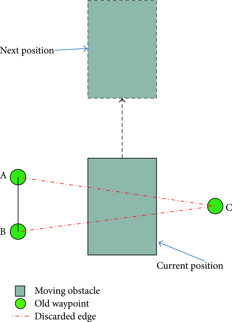
The update of waypoint graph when an obstacle moves in the region. No need to create the new waypoints and edges in the simplest way.

5.3. Prediction of Moving Obstacles

The prediction of the moving of the obstacles is important for the pathfinding especially for the emergency applications such as the fire evacuation. For both categories of moving obstacles, it is important to predict their possible locations in later several units of time; then the path should be revised to bypass the affected areas. For the second category of moving obstacles, further work is also needed to utilize the reenabled waypoints and edges when the obstacles go away.

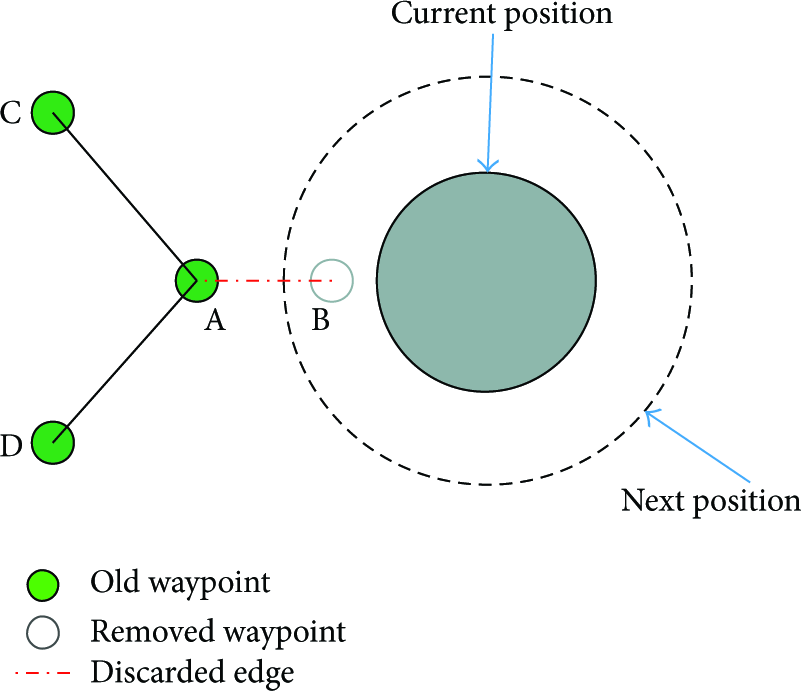
As shown in Figures 8 and 9, A will go to B since it is the shortest edge it can go, which is quite dangerous in the fire evacuation application since it is a direction towards the fire. Instead, the person in A should choose other places such as C or D in Figure 8 and E in Figure 9, based on the prediction of the motion of the fire in the near future.

Figure 8

Motion prediction of regular obstacles.

Figure 9

Motion prediction of irregular obstacles.

It is noted that the prediction of moving obstacles is quite difficult. The obstacles are with regular shape (e.g., Figure 8) or irregular shape (e.g., Figure 9) and the speed of their parts can be different. For the emergency applications, it is preferred to adopt the conservative way to predict the motions.

6. Path Finding

Based on the waypoint graph, we illustrate our algorithm to find the path in the dynamic environment. Generally speaking, the pathfinding can be categorized into two types, global approaches and local approaches.

The global approaches compute the whole path at the beginning and then go through that path step by step. The algorithms including Dijkstra [24], Floyd [25], A ${}^{*}$ [26], Any-angle algorithm [16], and others [27, 28]. During pathfinding, the localization technique [29, 30] can be used for the object to determine its current status. These approaches lack flexibility in the dynamic environment since the change of waypoint graph will cause the recomputing of the path.

The other type is the local approaches. They embed the direction information into the underlying graph and the object determines its action in the next step in the real time. These approach is more tolerant to the dynamic change of the environment. We use this idea in this paper. The waypoint in the graph is set a weight which increases from the center to the exit. The path finding algorithm aims to find a path which is from the point that has smaller weight to the bigger one. Specially attention should be paid to solve the local blocking situation and keep away from the accident area.

An objects moves to the destination from the origin via a multistep process. Algorithm 1 describes how the object chooses the target place in its next step. Generally speaking, the object is directed constantly towards the destination based on the waypoint graph. The local trap problem is solved in this process.

Algorithm 1: Waypoint graph based pathfinding.

   Input: $$\mathrm{c}\mathrm{u}\mathrm{r}\mathrm{r}\mathrm{e}\mathrm{n}\mathrm{t}$$ , $$\mathrm{p}\mathrm{r}\mathrm{e}\mathrm{v}\mathrm{i}\mathrm{o}\mathrm{u}\mathrm{s}$$ , $$\mathrm{d}\mathrm{e}\mathrm{s}\mathrm{t}\mathrm{i}\mathrm{n}\mathrm{a}\mathrm{t}\mathrm{i}\mathrm{o}\mathrm{n}$$ , $$\mathrm{c}\mathrm{a}\mathrm{n}\mathrm{d}\mathrm{i}\mathrm{d}\mathrm{a}\mathrm{t}\mathrm{e}\mathrm{P}\mathrm{o}\mathrm{i}\mathrm{n}\mathrm{t}\mathrm{s}$$

   Output: target

(1)   if   current is close to destination and current.weight is max then

(2)     target = destination

(3)   end

(4)   if   $$|\mathrm{c}\mathrm{u}\mathrm{r}\mathrm{r}\mathrm{e}\mathrm{n}\mathrm{t}-\mathrm{p}\mathrm{r}\mathrm{e}\mathrm{v}\mathrm{i}\mathrm{o}\mathrm{u}\mathrm{s}|<\mathrm{d}\mathrm{i}\mathrm{s}\mathrm{t}\mathrm{T}\mathrm{h}\mathrm{r}\mathrm{e}\mathrm{s}\mathrm{h}\mathrm{o}\mathrm{l}\mathrm{d}$$   then

(5)     jamCounter++

(6)   else

(7)     previous = current

(8)     jamCounter = 0

(9)   end

(10) if   $$jamCounter<threshold$$   then

(11)    candidatePoints.remove(current)

(12)    put the points in candidatePoints that can be reached from current into reachable

(13)   foreach   point in reachable   do

(14)   if   $$point.weight<current.weight$$   then

(15)     reach.remove(point)

(16)    end

(17)   endfch

(18)   target = min(reachable)

(19)   target.chooseCount++

(20) else

(21)  put the points in candidatePoints that can be reached from current into reachable

(22)  target = min(reachable)

(23)  put the points that have the same weight with current into candidatePoints

(24)  target.chooseCount++

(25)  jamCounter = 0

(26) end

In this algorithm, we firstly explain the function min $()$ . It is determined according to three metrics, the distance from the source node, the weight, and the chooseCount. Each waypoint in the graph has a weight. The value is gradually increased from the origin to the destination. Given two points $p_{\mathrm{1}}$ and $p_{\mathrm{2}}$ , let $d_{\mathrm{1}}$ be the distance between $p_{\mathrm{1}}$ and current and $d_{\mathrm{2}}$ the distance between $p_{\mathrm{2}}$ and current; if the difference between $d_{\mathrm{1}}$ and $d_{\mathrm{2}}$ is significant (in our simulation, we select 5 m as the threshold), the output is the point with the maximal value of $d_{\mathrm{1}}$ and $d_{\mathrm{2}}$ . Otherwise, we further check the weight and output the one with the smaller weight. If they have the same weight, the output is the one that has the smaller chooseCount. This function is used to select the most appropriate target waypoint in each step.

We have several variables in our algorithm and their explanations are as follows.

• (i)

weight: the weight of a waypoint.

(ii)

candidatePoints: a set of waypoint candidates. Its initial value is all waypoints.

(iii)

current: current position of the object.

(iv)

previous: the position of object in the previous step.

(v)

target: the position where the object moves in the next step.

(vi)

destination: the destination of the object.

(vii)

chooseCount: the times that the waypoint has been chosen.

(viii)

jamCounter: a nonnegative integer variable that records the times of the object's blocking.

(ix)

distThreshold: the threshold to measure the distance that the objects move normally or get potential stuck.

(x)

threshold: the threshold by measuring the number of potentials stuck to infer real stuck.

In the algorithm, the input parameters include $current$ , $previous$ , $destination$ , and $candidatePoints$ , and the output result is target, the position where the object moves in the next step. At first, we check whether the object is near the destination and its weight is the maximal one. If it is held, target will be updated to destination and pathfinding process will be complete in the next step (lines $(1)\text{–}(3)$ ). Then we check the possible stuck situation in the moving. This is calculated based on the distance between current and previous. If it is smaller than distThreshold, the object probably gets stuck, and therefore jamCounter is increased by one (lines $(4)\text{-}(5)$ ). If not, we simply update previous and jamCounter (lines $(7)\text{-}(8)$ ). For robustness, we handle the stuck situation only if jamCounter is no less than threshold (lines $(21)\text{–}(25)$ ).

The normal case is processed in lines $(11)\text{–}(21)$ . First, we remove current from candidatePoints since it is already considered (line (11)). Second, all waypoints in candidatePoints that can be reached from current are put into the list reachable (line (12)). We only consider the points with larger weights by filtering the waypoints whose weight is smaller than current's weight from candidatePoints (lines $(13)\text{–}(17)$ ). Then target is updated to the one that is closet to current (line (18)). After that chooseCount of target is increased by one (line (19)).

If the object is stuck, we process it in lines $(21)\text{–}(25)$ . All waypoints in candidatePoints that can be reached from current are put into the list reachable (line (21)). In this case, the target is not selected according to the weight. Instead, we select the closet waypoint that can be reached as target (line (22)). We then add all the waypoints that have the same weight value with current into candidatePoints (line (23)). The chooseCount of target is increased by one (line (24)). After solving the stuck situation, we set jamCounter to 0 (line (25)).

7. Performance Evaluation

In this section, simulations are carried out to validate the effectiveness of the proposed approach. Specifically, we check the performance of waypoint graph operations, the performance of pathfinding, and the performance of prediction strategy.

We built a 1 : 1 planar map of a shopping mall near Wuhan University, Wuhan, China (Figure 1), as the test region, which resides in a 187.5 m × 112.5 m rectangle. The target object’ radius is set to 0.2 m. The sparsification parameter Δ is set to be 16, and the maximum edge length is set to be 20 m.

$\text{JBox}\mathrm{2}\text{D}$ is used in the simulation for visualizing the pathfinding process. $\text{JBox}\mathrm{2}\text{D}$ is a Java version of the open source physics engine $\text{Box}\mathrm{2}\text{D}$ . It can be used to do 2D rigid body physical movement simulation automatically based on the parameters such as gravity, density, friction coefficient, and elastic coefficient.

Simulations were conducted at a ideaPad Y410P laptop with Intel Core TM i5-4200M CPU @2.50 GHz, 4 GB RAM, and NVIDIA Geforce GT755 & Intel HD Graphics 4600 graphic card.

7.1. Performance of Waypoint Graph Operations

First, we compare the performance of our used waypoint graph (balanced waypoint graph) with other alternative waypoint graphs (minimal waypoint graph and brutal waypoint graph) in the initialization process. We refer to balanced waypoint graph as balanced WPG, minimal waypoint graph as minimal WPG, and brutal waypoint graph as brutal WPG for short in the rest of discussion in this paper. The result is shown in Table 1.

Table 1

The structure and initialization time of different waypoint graphs.

Method	Balanced WPG	Minimal WPG	Brutal WPG
	#number
Edges	102	93	152
Waypoints	91	78	40
	#time (ms)
WCG	1	1	1
WVC	19	20	18
CWGC	17	16	15
IGS	14	29
EI	2	1
Total	53	67	34

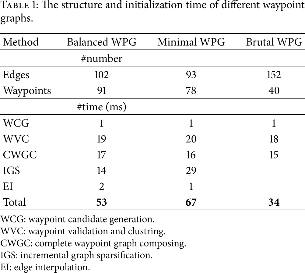
WCG: waypoint candidate generation.

WVC: waypoint validation and clustring.

CWGC: complete waypoint graph composing.

IGS: incremental graph sparsification.

EI: edge interpolation.

According to the table, making the graph sparse causes additional time overhead in the initialization process, but the overhead is small compared with the time of the whole process. Compared with the brutal WPG, balanced WPG and minimal WPG reduce more than 33 percent of edges in the waypoint graph, which can speed up pathfinding operation and save memory storage. The edge reduction also helps to generate less waypoints during the edge interpolation process. On the other hand, balanced WPG and minimal WPG create new waypoints (due to edge interpolation), which are about twice as the ones generated by brutal WPG. Since the pathfinding algorithm we used is edge-based algorithm, the waypoint graphs generated by balanced WPG and minimal WPG are more appropriate.

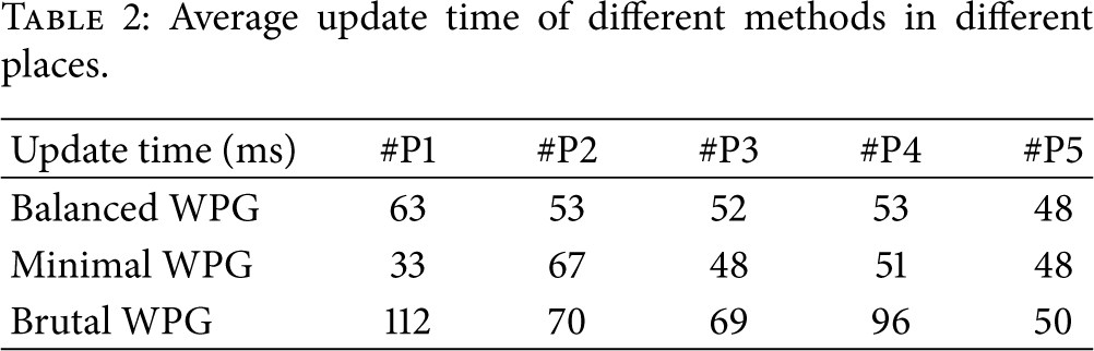
Then we check the performance of the approaches when adding an obstacle and then removing it at 5 distinctly different places (P1, P2, P3, P4, and P5) on the map. The added obstacle is set to be a constant-sized rectangle. The configuration can be seen in Figure 10. The tests in each place are conducted several times to get the average value. The results are shown in Table 2. We can see that minimal WPG takes the least time. Brutal WPG does not control the edge length of waypoint graph; thus it cannot determine the size of affected area. Therefore it cannot conduct local update and take more time compared with other two methods.

Table 2

Average update time of different methods in different places.

Update time (ms)	#P1	#P2	#P3	#P4	#P5
Balanced WPG	63	53	52	53	48
Minimal WPG	33	67	48	51	48
Brutal WPG	112	70	69	96	50

Figure 10

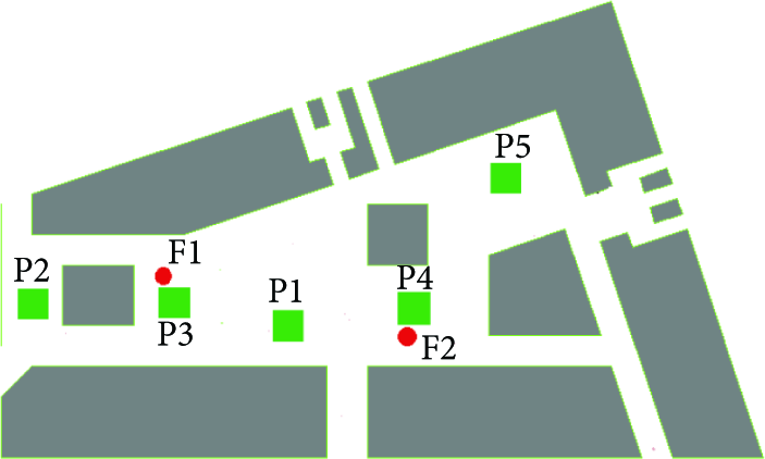
Configuration of the simulations.

7.2. Performance of Pathfinding

We further test the performance of pathfinding under different waypoint graphs. We used two kinds of approaches in the test. The first one, A ${}^{*}$ algorithm with Euclid heuristic, belongs to global pathfinding approaches. The second one, our approach discussed in Section 4, belongs to local pathfinding approaches. The operation time and the path quality before and after obstacle altered are compared. Path quality is measured by path length ratio, the length of the path over that of the theoretical shortest path. The theoretical shortest path can be obtained by applying Dijstra on brutal WPG. An example of waypoint graph when an obstacle is added and removed is shown in Figure 11. For each kind of the two approaches, we conduct pathfinding 1000 times for one which we choose the leftmost waypoint as the origin and the rightmost waypoint as the destination.

Figure 11

Waypoint graph and pathfinding result of balanced WPG. The black hollow rectangle denotes the obstacle. The blue dots are waypoints, and the green lines are edges among waypoints. The red lines represent the pathfinding result. The results are before new obstacle insertion (a), after obstacle insertion (b), and after obstacle removal (c), respectively.

The results when using A ${}^{*}$ algorithm are shown in Table 3. It shows that the pathfinding time when using balanced WPG and minimal WPG is much less than brutal WPG. Although brutal WPG generates the graph that contains the least waypoints, the average degree of their waypoints is the highest. Since the number of edges dominates the complexity of pathfinding, balanced WPG and minimal WPG have better performance.

Table 3

The operation time and path length ratio of different waypoint graph (A^* approach).

	Balanced WPG	Minimal WPG	Brutal WPG
Pathfinding time (ms)	2.71	2.02	3.43
PLR before insertion	1.068	1.130	1.014
PLR after insertion	1.043	1.092	1.003
Average PLR	1.056	1.111	1.008

PLR: path length ratio.

Brutal WPG is based on the complete waypoint graph, so its pathfinding result is almost the same as the real shortest path. Minimal WPG has trimmed edges as many as possible by making each point have at most one incident edge in one of four directions, which may remove important edges and cause path quality loss. Its result is about 11 percent longer than the shortest path. Balanced WPG carefully trades off the execution time and the quality of path. Its result is less than 6 percent longer than the shortest path.

The results when using our approach are shown in Table 4. It is similar that the pathfinding time when using balanced WPG and minimal WPG is much less than brutal WPG. The difference exists that the path length ratio under brutal WPG is larger than that of balanced WPG and minimal WPG. This is because local approaches like our approach determine the moving objective in each step based on local information, so a larger number of edges in brutal WPG may result in necessary go-and-return operations and larger length of path. It shows that the path length ratio under minimal WPG is the least among the three waypoint graphs, which validates the effectiveness of our design quite well.

Table 4

The pathfinding time and path length ratio of different waypoint graph (our approach).

	Balanced WPG	Minimal WPG	Brutal WPG
Pathfinding time (ms)	3.37	3.12	4.14
PLR before insertion	1.469	1.491	1.889
PLR after insertion	1.555	1.576	2.612
Average PLR	1.055	1.534	2.250

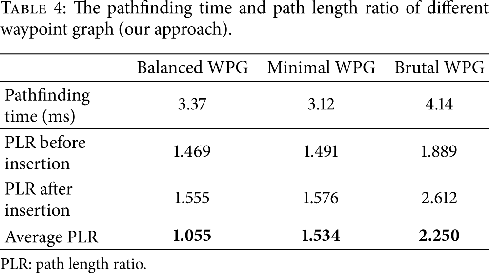
PLR: path length ratio.

7.3. Performance of Prediction Strategy

We conduct simulations to check the performance of the prediction strategy used in this paper. Two categories of obstacles are used for the experiments. One is a fire that expands its occupied area to the neighborhood in a constant speed. The other is a dangerous object that changes its location to others in a constant speed.

We first check the evacuation time of our approach when a fire accident occurs. We vary the number of people from 100 to 600 in the tests. There may be one or two fires in the region, whose places can be F1 or F2 as shown in Figure 10. The result is shown in Figure 12. It can be seen that the evacuation time when there are two fires is larger than that when there is just one fire. This is because more fires in the region are more likely to make the person take a longer path to guarantee safety. The evacuation time when we use prediction strategy is larger than that when we do not use prediction strategy. The reason is that the prediction tends to find a longer but safer path for the person, compared with no prediction. It is noted that the evacuation time under no fire situation is larger than that under one fire situation. This is because some slow people cause a large value of evacuation time in the fire-free situation, but such people may be killed in the fire condition which reduces the average evacuation time.

Figure 12

The evacuation time in different situations.

In the following four simulations, we assume that there are 300 persons in the region. We set the prediction distance of the fire to 8 m and check the number of victims under different speeds of fire. The result is shown in Figure 13. According to that figure, the number of victims caused by the fire increases when the speed of fire increases. It increases relatively slower when the speed of fire increases from 1 m/s to 4 m/s and then faster when it further increases from 4 m/s to 6 m/s. The number of victims when using prediction approach is less than that not using prediction approach in all speeds of fire. It is because a proper path can be suggested to the persons to avoid the fire in advance using prediction approach. It is especially effective when the speed of fire is high. When the speed of fire is 6 m/s, there are 223.6 victims (casualty rate 0.745) if prediction is not used and 186.4 victims (casualty rate 0.621) if prediction is used. There is a 16.6% reduction in the casualty rate.

Figure 13

The performance of prediction approach in different speeds of fire.

For the dangerous objects, we set the prediction distance of it to 4 m and check the number of victims under different speeds. The result is shown in Figure 14. Similar to the case of fire, the number of victims when using prediction approach is less than that when not using it in all speeds. We only report the results when the dangerous object has a speed no less than 3 m/s, because there is nearly no victim if using prediction approach when its speed is less than 3 m/s. The gap in casualty rate between using prediction and not using prediction is stable. When the speed of dangerous object is 6 m/s, there are 12.8 victims (casualty rate 0.043) if prediction is not used and 3.6 victims (casualty rate 0.012) if prediction is used. There is a 72.1% reduction in the casualty rate.

Figure 14

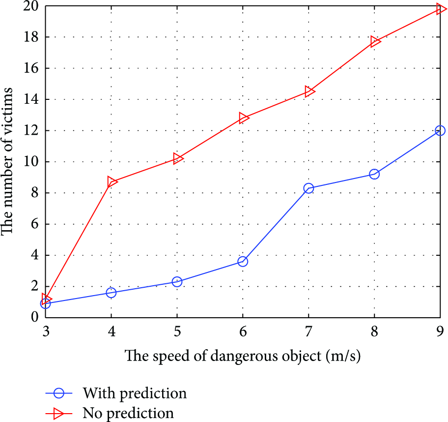
The performance of prediction approach in different speeds of dangerous object.

We further show how much we need to predict the obstacles to get a good performance. We vary the prediction distance of the obstacles to check the performance. The results are shown in Figures 15 and 16. For the first category of obstacles such as fire, it shows that the impact of prediction distance varies in different speeds of fire. When the speed of fire is quite low (e.g., 2 m/s) or quite high (e.g., 4 m/s), the prediction is not so sensitive to the specific prediction distance. It can be explained that when the speed of fire is quite low, the object always can find a proper path to escape, and when the speed of fire is quite high, the probability that the person can escape is quite little although it can avoid fire temporally. It is noted that the difference still exists between using prediction (the prediction distance > 0 m) and not using prediction (the prediction distance = 0 m). The prediction distance has obvious impact on the pathfinding when the speed of fire is moderate (e.g., 3 m/s). The number of victims reaches the minimal value when the prediction distance is 3 m. When prediction distance is less than 3 m, the people are likely be caught by fire. When the prediction distance is larger than 3 m, the people miss the shortest path to leave the dangerous areas.

Figure 15

The performance of prediction approach in different prediction distances of fire.

Figure 16

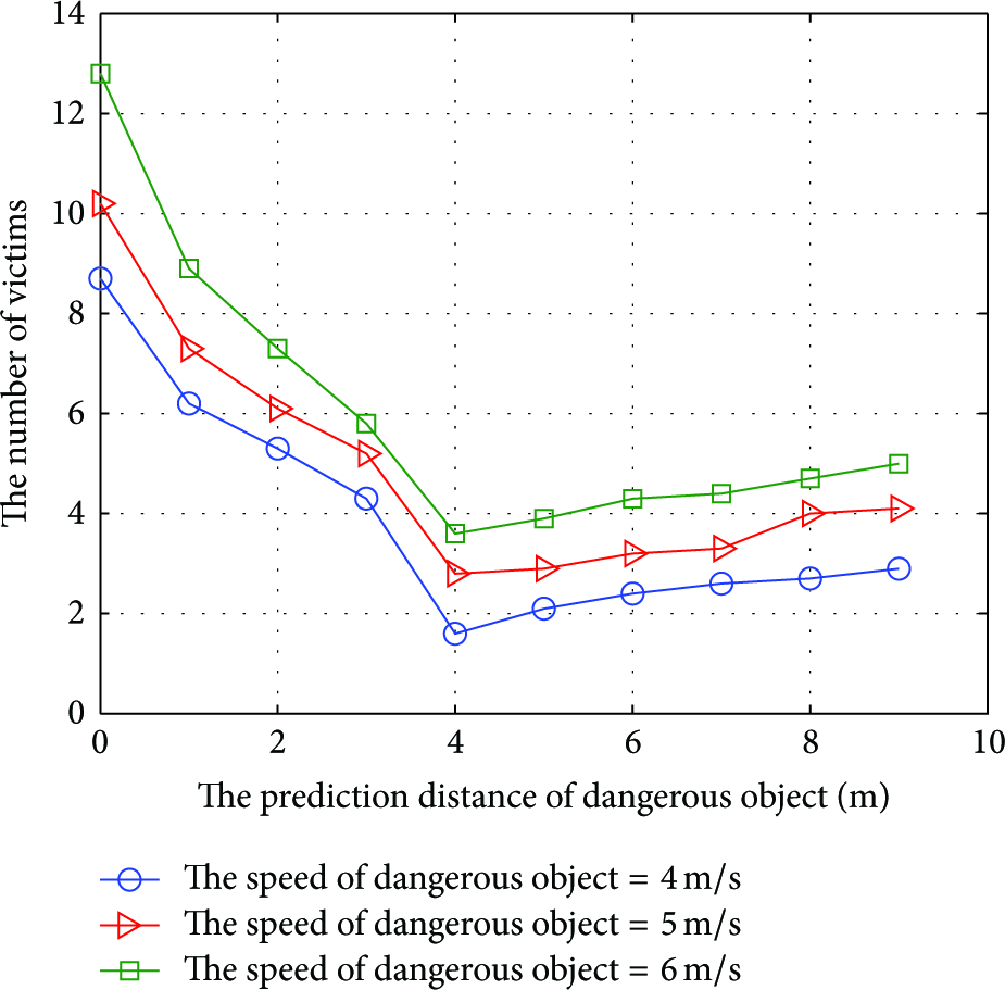
The performance of prediction approach in different prediction distances of dangerous object.

The impact of prediction distance is more obvious for the second category of obstacles. The result is shown in Figure 16. This is because this category of obstacles has a smaller size and the occupied area is constant compared with the first category of obstacles. Therefore a proper prediction distance can make the person avoid the dangerous objects and the effect of missing the shortest path is not so serious. This is can be seen that the number of victims is greatly decreased when the prediction distance of dangerous object increases from 0 m to 4 m and increases quite slowly when the prediction distance of dangerous object increases from 4 m to a larger value. Let us check the performance under the speed of 5 m/s, the number of victims is 2.8 when the prediction distance of the dangerous object is 4 m, and the number of victims is 7.3 when the prediction distance of dangerous object is 1 m. There is a 61.6% reduction in the casualty rate.

8. Conclusion

In this paper, we investigated the waypoint graph based pathfinding problem in the dynamic environment. The frequent change of environment causes large computation overhead and long latency of pathfinding in such scenario. We propose a new fast approach to address such problem. We improve the waypoint graph approach by reducing the number of waypoints and edges. Based on that, we design a local method to handle the dynamic change and then pathfinding in the dynamic environment. The waypoint graph is locally updated based on the prediction of the motions of the moving of obstacles and local calculation of affected areas. We have conducted extensive simulation to validate the effectiveness of the approach. The results show that the proposed approach outperforms existing approaches in terms of the response time and rescue rate in the emergency applications. In the future, we plan to design a real-time approach to achieve pathfinding in the dynamic environment. We also want to extend this work to consider the distributed map detection in an unknown environment.