Sage Journals: Discover world-class research

Abstract

Providing reliable communication represents one of the major barriers to wireless sensor networks. In this paper, we propose a fault-tolerant tableless routing protocol called E-cube⁺, inspired from e-cube routing protocol, to support intelligent rerouting. A range of fault-tolerant routing properties of E-cube⁺ (such as loop-freeness, failure recovery guarantees, and bounded latency) have been derived and analyzed. Experiment results also show that E-cube⁺ is able to route data properly without complicated and energy-intensive routing table lookup processes even when node failures occur.

1. Introduction

Due to the constraints of available resources in WSN [1–4], sensor nodes are subject to relatively high fault rates. When certain sensor nodes fail, the communication function of the WSN would be interrupted, resulting in a low transmission efficiency of the entire network. In order to mitigate the impact of the limited resource constraints imposed on WSN, a better routing protocol that can tolerate node failures while keeping the transmission efficiency of the entire WSN is required. A fault-tolerant routing protocol can significantly improve the reliability and stability of the network system. However, some resource constraint characteristics (e.g., limited energy supply and small memory) make the design of fault-tolerant routing protocols for the WSN a challenging task.

For a healthy WSN without node failures, a routing algorithm called e-cube [5] is widely used in many WSN applications [6–8]. The e-cube is a dimension-ordered deterministic routing algorithm based on the hypercube model, which is easy to implement in parallel computer architectures. The conventional e-cube routing algorithm has many desired properties (such as low latency and loop freeness), but it is not able to work well under an injured hypercube, which has faulty links/nodes.

There are many existing protocols that can be used for WSNs that are fault-tolerant [9–14]. However, these protocols are unable to overcome the resource constraints of WSNs, because most protocols require a large memory space for the routing and power-consuming table lookup operations. In large-scale WSN, the impact of these requirements is more significant. Thus, in this paper, we explore the design of a memory-efficient and fault-tolerant routing protocol.

To dynamically adapt to network failures or congestions, Gaughan and Yalamanchili [15] proposed backtracking protocols to find an alternative path in a depth-first manner. In such cases, sensors must reestablish the routing information and cannot achieve an immediate path swap, which may increase the transmission cost (such as long latency and packet loss). Chen and Shin [16] used an n-bit vector tag to keep track of the abundant dimensions which are used to calculate alternative paths bypassing faulty components. The n-bit vector tag inevitably introduces communication overhead and additional computation. In the safety vector approach [17], each sensor node needs to maintain a vector indicating the awareness of the status of other nodes. This raises some communication and computation issues simultaneously, which make WSN routing design even more challenging. As such, these methods are not suitable for WSNs due to limited resources (such as CPU power or memory) and high latency problems.

In this paper, we propose a fault-tolerant routing protocol named E-cube⁺, which covers the e-cube original spirit and can be implemented in a hierarchical routing network. E-cube⁺ is able to compute the alternative backup paths without routing table lookup to recover the WSN from network failures. The proposed scheme offers a quick reroute functionality with low processing and memory overhead for the WSN. The salient features of E-cube⁺ are listed as below.

(1) No Routing Table. In the E-cube⁺ algorithm, every node finds the next hop to the destination using simple bit operations. Except for the storage of its own label and related proxy labels, it saves significant memory space and avoids power- and time-consuming routing table lookup. Unlike e-cube routing algorithm, E-cube⁺ routing protocol presented in this study not only forwards the packets but also effectively reroutes the packets by obtaining an alternative path to the destination node.

(2) Failure Recovery Guarantees. E-cube⁺ is capable of finding backup paths with ( $m - 1$ ) guarantee link failures under m-dimensional complete hypercube (m-DCH) structure. An M-dimensional complete hypercube is a graph which comprises $2^{m}$ nodes, each with m bidirectional links connecting to m neighbors. In comparison, the traditional static routing methods simply store only one or two backup paths beforehand in the routing table. When multiple nodes are damaged, the backup path may fail, resulting in missed packets and wastage of the resources of entire wireless sensor network.

(3) Bounded Latency. In m-DCH, every pair of nodes has a bounded length m due to the inherent property of the hypercube model. In addition, when a single node fails, the worst case message transmission latency (MTL) in terms of hop count is a fixed number of m (hops). The bounded latency for real-time packet transmission is a nice property, since there will not be out-of-control variation during data transmission.

2. Related Work

Fault tolerance is to ensure that the system still works as expected even failures occur. In fault-tolerant computing, some algorithms are able to produce a correct output or a quasicorrect output when in presence of memory faults. Many researches adopted the memory error detection/correction code, such as cyclic redundancy check (CRC), hamming code, and checksum, for soft errors in a memory system by little overhead of code size as there exist memory errors and mal-packet problems [18–22]. In data communication area, timeout detection and recovery (TDR) is a popular solution for resolving fault tolerance related issues. If the acknowledgement is not received by the sender within the timeout period, the data would be retransmitted [23].

Ad hoc on-demand distance vector routing (AODV) [24] and dynamic source routing (DSR) [25] are two simple and widely used routing protocols in WSN. Both protocols are efficient routing protocols to establish the shortest path with low power consumption. However, the nature of WSN topology is dynamic due to many factors including limited power supply of the sensor nodes, unstable wireless link quality, and physical damage. The above primitive single-path routing approaches are not well suitable for WSN because the source node triggers the alternative path discovery operation and may cause further unacceptable delay and overhead for data transmissions when the primary path fails to forward data towards the sink. Thus, multipath routing approach is deemed an effective technique to meet the fault tolerance demands. A set of multiple paths between the source nodes and the sink are stored to provide constructed alternative paths as the backup paths in case of the primary path failure. By summarizing previous typical multipath-based schemes such as [26–33], we introduce four phases of the multipath routing procedures.

(i)

Phase 1: locate a set of intermediate nodes to establish paths from the source node to the sink node based on different criteria (e.g., link-disjoint [26], node-disjoint [27], or partially disjoint paths [28]).

(ii)

Phase 2: choose the right number and efficient paths from the set of path disjointedness discovered at Phase 1. Those selected paths are ready to transmit the data when the primary path fails. Of course, the path selection technique has a big impact on the fault tolerance capabilities [29]. For example, energy-adaptive multiple paths routing algorithm (EMRA) [30] considers energy consumption a part of the cost functions to be used for selecting fault-tolerant multiple paths.

(iii)

Phase 3: activate the chosen paths from Phase 2 and start the data transmission across selected paths. There are several options to choose from when to deliver data (such “as one path at a time” [31], “simultaneous use of K-paths” [32], and “all paths at the same time” [33]). In “one path at a time approach”, source node uses only one path to transmit data and switches to another alternative path when failure occurs. On the other hand, the source node uses K distinctive paths or all paths for data transmission concurrently [32, 33]. The source node is able to utilize all activated paths sending multiple copies of the same packet over all paths in order to recover if some paths fail.

(iv)

Phase 4: reinitiate path discovery process to accommodate the dynamic topology changes when a link/node fails.

In summary, multipath approaches can find a set of alternative paths via path recovery process. When the primary path failure occurs, the intermediate node will reroute the packet via the alternative path. The aforementioned methods construct the multipath routes through broadcasting message to the whole network in order to collect all information (such as residual energy, hop counts, and the signal strength) from the neighboring nodes and create the forwarding table for data transmission.

WSN typically involves hundreds or even thousands of sensors. Other distinctive features of wireless sensor networks are CPU capability and low-memory capacity. To our best knowledge, multipath routing protocols do not address the resource constraints of the sensor (such as CPU and storage). However, they need to process all information collected from the enormous number of sensor nodes, store all multipath routing information, and look up the routing table for every packet. As such, energy-aware multipath techniques usually suffer from broadcasting message overhead and a lack of scalability. To address this resource constraint issue of the sensor, the proposed E-cube⁺ routing algorithm applies simple bit operations in every node to determine the next hop to the destination without the routing table lookup.

We summarize the differences among E-cube, multipath routing based EMRA [30], and the proposed approach (E-cube⁺) at Table 1.

Table 1

Comparison with various approaches.

	e-cube [5]	E-cube⁺	EMRA [30]
Routing type	Deterministic routing	Deterministic routing	Adaptive routing
Forwarding mechanism	2 selective virtual channels	2-selective-link hop routing	Multiple paths
Traffic distribution	Nodes with label of 1-bit difference are reachable	Nodes with label of 1-bit difference are reachable	Disseminate data along chosen paths by lowest delay, energy consumption, or disjoint path
Loop-freeness	Yes	Yes	Not addressed
Routing table	Tableless	Tableless	Yes
Backtrack when it fails to forward	No	Yes	No
Failure recovery guarantees	Single failures	( $m - 1$ ) guarantee link failures under m-DCH structure	No
Bounded latency	No	Yes	No
Reinitiate path discovery overhead	High	Low	High

3. Fault-Tolerant E-Cube⁺ Routing

We propose a fault-tolerant tableless routing protocol with low energy cost and low memory requirement called E-cube⁺ routing protocol, which extends e-cube routing protocol to handle the faulty conditions. For better describing the proposed E-cube⁺ algorithm, here we define some notations that will be used throughout this paper (as shown in Table 2).

Table 2

Notations and descriptions in E-cube⁺ model.

Notation	Description
$H (N_{i}, N_{j})$	The Hamming Distance between labels of the nodes, $N_{i}$ and $N_{j}$ . For example, $H (010,101)$ = 3.
$N_{S}$	The source node.
$N_{D}$	The destination node.
$N_{C}$	The current node.
$N_{N}$	Next node of $N_{C}$ for routing.
$\overset{⊥}{N_{C}^{i}}$	The presentation of inverting the ith bit of the $N_{C}$ 's label.
$U (m, k)$	The hop count for message transmission for upper bound estimation in the worst case when there exist k node failures in m-DCH network topology.
$L (l_{i}, l_{j})$	This Boolean function indicates whether there is a routing loop from the node of the ith level ( $l_{i}$ ) to the node of the jth level ( $l_{j}$ ) in all possible routing paths. For instance, L( $l_{1}$ , $l_{m + 1}$ ) = 0 that means loop-free routing from the source of $l_{1}$ to the destination of $l_{m + 1}$ .

3.1. Packet Header Format

As mentioned in the above description, E-cube⁺ uses the bit arrays of the vertices in the hypercube model as the labels for the nodes in the WSNs. The E-cube⁺ protocol combined with the packet header will be able to run the routing algorithm. The packet header format (as Figure 1) in the E-cube⁺ protocol is defined as follows.

Figure 1

Packet header format of E-cube⁺ in IEEE 802.15.4.

(i) Length. It is a byte to represent the length of each E-cube⁺ label and to imply the total length of E-cube⁺ packet header (one byte + five times of the length of each E-cube⁺ label).

(ii) Genuine Source Label (GSLabel). When the number of sensor nodes exceeds a complete hypercube, the extra nodes can use other nodes as their proxy for transmission. This field is for the source node, and the corresponding proxy node uses the source label field. If no proxy is used, GSLabel equals 0.

(iii) Genuine Destination Label (GDLabel). Similar to the GSLabel, this field is for the destination node. The corresponding proxy node uses the destination label field. If no proxy is used, GDLabel equals 0.

(iv) Source Label (SrcLabel). It is source node label or the proxy label of the real source.

(v) Destination Label (DstLabel). It is destination node label or the proxy label of the real destination.

(vi) Intermediate Label (ImdLabel). It is the current node label before transmission to the next node.

3.2. Routing Algorithm

Based on a hypercube model, the well-known e-cube or “left-to-right” (LR) routing algorithm routes a packet from source to destination by traversing the differing dimensions in a left-to-right order. However, e-cube routing algorithm does not address network link failure issues completely. To address this issue further, the proposed E-cube⁺ routing algorithm applies simple bit operations in every node to determine the next hop to the destination. Each node may perform two main functions: getLeftN and getRightN. The former function determines the next hop ( $N_{N}$ ) on the principal working path to the destination ( $N_{D}$ ), and the latter determines the next hop on the backup path. The function getLeftN first performs an exclusive OR (XOR) operation on the label representing the current node ( $N_{C}$ ) and the label representing the destination node ( $N_{D}$ ). Then, it determines from left to right the position i of the first nonzero bit as shown in (1), called LSB function. Finally, it inverts the ith bit of the current node label and obtains the label for the next node, as shown in (2) where $N_{C}$ also stands for the label (binary presentation of node identification) of the current node, $N_{D}$ represents the label of the destination node, and LSB is the left significant bit function which returns the position i of the first nonzero bit from left to right. Consider

\begin{matrix} i \equiv LSB (N_{C} \oplus N_{D}), \end{matrix}

(1)

\begin{matrix} N_{N} = \overset{⊥}{N_{C}^{i}} . \end{matrix}

(2)

For instance, the binary presentation of $N_{C}$ 's identification is 01010, the binary presentation of $N_{D}$ 's is 10110, and then the default next hop $N_{(11010)}^{1 -Hop}$ is determined (at $N_{C}$ ) as $i \equiv LSB (01010 \oplus 10110) = 1$ and $N_{N} = \overset{⊥}{N_{C}^{i}} = \overset{⊥}{(\underline{0} 1010)_{}^{i = \underline{1}}} = 11010$ (convert-bit-position order from left).

If E-cube⁺ detects communication problem from the current node to destination node via node $N_{N}$ (which is selected using the getLeftN function), it will perform the getRightN function to determine the first nonzero bit i from right to left using the RSB function, as shown in (3). The next hop node label is derived by inverting the ith bit of the current node label, as shown in (2). Please note the bit-position direction for $N_{N} = \overset{⊥}{N_{C}^{i}}$ is different according to LSB or RSB function, but we only define a notation of $N_{N} = \overset{⊥}{N_{C}^{i}}$ . Consider

\begin{matrix} i \equiv RSB (N_{C} \oplus N_{D}) . \end{matrix}

(3)

The E-cube⁺ routing algorithm is illustrated in Algorithm 1. In a wireless sensor network equipped with E-cube⁺, during data transfer between nodes, every node in the process performs the following routing steps.

(i)

Line 03: receive the packet (Pkt).

(ii)

Lines 04–11: if current node is the destination, there are three cases. (1) If there is a proxy before the destination (its label is Pkt.DstLabel), pass the packet to the upper-layer protocol; (2) the current node is the destination, and there is no other node as the proxy; (3) if it is the proxy of other nodes, then broadcast the packet to its proxy member.

(iii)

Lines 13–16: call getLeftN and get the next hop of the main routing path; then put its own label in the Pkt.ImdLabel, and forward the packet to the next hop.

(iv)

Lines 19–22: call getRightN and get the next hop of the backup path; then put its own label in the Pkt.ImdLabel, and forward the packet to it.

(v)

Lines 25–29: start backward routing. If it is already at the source node, discard the packet.

Algorithm 1: The E-cube⁺ routing algorithm.

(01) MyID = selfID();

(02) while (TRUE) {

(03) Pkt = receivePacket();

(04) if (MyID == Pkt.GDLabel) // Genuine receiver behind a proxy

(05) sendUpperLayer(Pkt);

(06) else if (MyID == Pkt.DstLabel) {

(07) if (Pkt.GDLabel == 0) // Genuine receiver does not have a proxy

(08) sendUpperLayer(Pkt);

(09) else // Current node is a proxy and broadcasts in its domain

(10) broadcastProxyMember(Pkt);

(11) }

(12) else { // Forward at intermediate nodes

(13) LeftN = getLeftN (MyID, Pkt.DstLabel); // Main path

(14) if ((LeftN != Pkt.ImdLabel) && Link(LeftN)){

(15) MarkPacketImd(MyID, Pkt);

(16) sendPacket(LeftN, Pkt);

(17) }

(18) else {

(19) RightN = getRightN (MyID, Pkt.DstLabel); // Backup path

(20) if (Link(RightN)) {

(21) MarkPacketImd(MyID, Pkt);

(22) sendPacket(RightN, Pkt);

(23) }

(24) else { // Forwarding path failed

(25) if (myID == Pkt.SrcLabel) // Drop as no available path

(26) dropPacket(Pkt);

(27) else { // Backward to previous node

(28) MarkPacketImd(MyID, Pkt);

(29) backwardPacket(PreviousNode, Pkt);

(30) $}}}}$

In summary, the working path is decided by the routing functions based on E-cube⁺ routing algorithm (as shown in Algorithm 1). Routing path is determined based on the labels of the destination node and that of current node. Upon receiving the packet, the current node obtains the next hop of the principal working path via executing the Lines 13–16. If E-cube⁺ detects a communication problem to the next hop of the principal working path, it would execute the routing logic (Lines 19–22) to find the next hop of the backup path. If both next hops of the principal working path and the backup path are not reachable, the current node would perform the backtracking procedure to send the packet back to the previous node (Lines 25–29).

3.3. Example

For clear explanation, we will use a 5-DCH network topology as an example and demonstrate three cases with different failure nodes to explain the transmission of a packet from the source node $N_{\{01010\}}$ to the destination node $N_{\{10110\}}$ . The process is shown in Table 3.

Table 3

A tracing example of E-cube⁺.

Case	Current node	getLeftN	getRightN	DstLabel
Case I: no failure node	01010	$11010$		10110
	11010	$10010$		10110
	10010	$10110$		10110
	10110

Case II: node 10010 fails	01010	$11010$		10110
	11010	$10010$	$11110$	10110
	11110	$10110$		10110
	10110

Case III: node 10010 and node 11110 fail	01010	$11010$		10110
	11010	$10010$	$11010$ (backtrack)	10110
	01010		$01110$	10110
	01110	$11110$	$00110$	10110
	00110	$10110$		10110
	10110

Case 1 (normal routing with no failure nodes).

$N_{\{01010\}}$ executes the algorithm Lines 13~16. From getLeftN, (LSB(01010 $\oplus$ 10110) ≡ 1 and inverting the 1-bit from left of the current node label 01010 to be 11010), the algorithm knows that the next hop is $N_{\{11010\}}$ . It puts its own label into the Pkt.ImdLabel, and then forwards the packet to the next hop. Next, $N_{\{11010\}}$ and $N_{\{10010\}}$ also execute Lines 13~16 to pass the packet to $N_{\{10110\}}$ . Then, $N_{\{10110\}}$ executes Lines 06~08 and identifies itself as the real destination and sends the packet to the upper-layer protocol.

Case 2 (backup routing with a single failure node).

$N_{\{01010\}}$ executes Lines 13~16, puts its own label into Pkt.ImdLabel, and then forwards the packet to $N_{\{11010\}}$ . Next, $N_{\{11010\}}$ also executes the getLeftN command but realizes that $N_{\{11010\}}$ has failed and, thus, goes to Lines 19~22. From getRightN (RSB(11010 $\oplus$ 10110) ≡ 3 and inverting the 3-bit from right of the current node label 11010 to be 11110), it knows that the next hop is $N_{\{11110\}}$ and forwards the packet to $N_{\{11110\}}$ . $N_{\{11110\}}$ executes Lines 13~16 and passes the packet to $N_{\{10110\}}$ . $N_{\{10110\}}$ executes Lines 06~08 and sends the packet to the upper-layer protocol.

Case 3 (backward routing during multiple failures).

$N_{\{01010\}}$ executes Lines 13~16, puts its own label into Pkt.ImdLabel, and then forwards the packet to $N_{\{11010\}}$ . Next, $N_{\{11010\}}$ is informed that the next hop is the failed $N_{\{10010\}}$ or $N_{\{11110\}}$ (i.e., the main path and the backup path both fail) and, thus, runs Lines 28~29 for backward routing the packet to node $N_{\{01010\}}$ . When $N_{\{01010\}}$ calls getLeftN and realizes that the packet has been back routed (since Pkt.ImdLabel equals $N_{\{11010\}}$ ), it executes Lines 19~22. Through getRightN, it knows that the next hop is $N_{\{01110\}}$ and forwards the packet to $N_{\{01110\}}$ . Next, $N_{\{01110\}}$ executes getRightN to transmit to $N_{\{00110\}}$ because its getLeftN is the failed $N_{\{11110\}}$ as Link(LeftN) = Null. Then $N_{\{00110\}}$ executes getLeftN to get $N_{\{10110\}}$ and sends the packet to $N_{\{10110\}}$ .

3.4. Property

In this section, we first perform the latency bound analysis for the fault tolerance capability of E-cube⁺ and then show the loop-free routing property for data transmission as in Theorems 1 and 2, respectively. Under m-DCH topology, the proposed E-cube⁺ method can guarantee successful transmission under $m - 1$ node failures. Moreover, the upper bound of message transmission latency (MTL) in terms of hop count is analyzed under the m-DCH model. The worst case analysis is based on the Hamming Distance of source node and destination node, which is equal to m. Through the analysis of the worst case of $m - 1$ node failures, the upper bound of MTL for successful message transmission can be presented as in Theorem 1.

Theorem 1.

When there exists k node failures in m-DCH network topology, the upper bound of MTL is $U (m, k) = m + 2^{(k + 1)} - 2 k - 2$ .

Proof.

The formula can be proved by mathematical induction as follows.

Step 1. We first prove that the statement is true for $k = 0$ . The number of hop counts for message transmission is m when there is no node failure; that is, $U (m, 0) = m$ . Since the Hamming Distance between source node and destination node is m (e.g., $H (010, 101) = 3$ ; $H (N_{S}, N_{D}) = m$ ), the MTL is equal to the value derived from the formula $U (m, 0) = m + 2^{(0 + 1)} - 2 \cdot 0 - 2 = m$ .

Step 2. We prove that if the statement is true for $k = m - 2$ , then it is also true for $k = m - 1$ . Given that, $U (m, m - 2) = m + 2^{(m - 2 + 1)} - 2 \cdot (m - 2) - 2 = 2^{(m - 1)} - m + 2$ is true. Let $R_{i, j}$ denote a sensor node along with the path from the source node ( $N_{S}$ ) to the destination node ( $N_{D}$ ) where i presents level and j indicates the sequence between the nodes at the same level i by the E-cube⁺ routing algorithm (as shown in Figure 2). In the worst case scenario for $m - 2$ node failures, there are two phenomena: (1) $N_{D}$ is m levels away from $N_{S}$ , which implies that $N_{S} = R_{1,1}$ and $N_{D} = R_{m + 1,1}$ . (2) The failure node sequences are $R_{m, j}$ and $1 \leq j \leq m - 2$ .

When $k = m - 1$ , the sensor node $R_{m, m - 1}$ fails, we can derive

\begin{array}{l} U (m, m - 1) = U (m, m - 2) - 2 \\ + (m - 2) + 1 + U (m - 1, m - 2) \\ = [m + 2^{(m - 2 + 1)} - 2 (m - 2) - 2] + [m - 3] \\ + [m - 1 + 2^{(m - 2 + 1)} - 2 (m - 2) - 2] \\ = [2^{(m - 1)} - m + 2] + [m - 3] + [2^{(m - 1)} - m + 1]    \\ = 2 \cdot 2^{(m - 1)} - m = 2^{m} - m . \end{array}

(4)

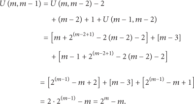
The E-cube⁺ produced routing path looks like Pascal's triangle, called Yang Hui's triangle in China, plus the final destination node. A brief explanation of the above derivation is listed as follows.

(i)

$U (m, m - 2) - 2$ : due to the failure of the last hop $R_{m, m - 1}$ , E-cube⁺　saves 2 hop counts at its previous hop ( $R_{m - 1, m - 2}$ ) in the routing path.

(ii)

$+ (m - 2)$ : E-cube⁺ backwards the packet from $R_{m - 1, m - 2}$ to $N_{S}$ .

(iii)

$+ 1$ : E-cube⁺ forwards the packet to next hop $R_{2,2}$ for the backup routing.

(iv)

$+ U (m - 1, m - 2)$ : the follow-up of the hop counts can be regarded the same as $m - 1$ -DCH with $m - 2$ node failures in the worst case.

Finally, the MTL inferred above is equal to the result of the formula according to $U (m, m - 1) = m + 2^{(m - 1 + 1)} - 2 \cdot (m - 1) - 2 = 2^{m} - m$ , so the inductive proof is complete.

Figure 2

Example of the transmission route from the source to the destination by E-cube⁺ under m-DCH for the worst case analysis.

Theorem 2.

The routing procedure of E-cube⁺ algorithm is loop-free, denoted as $L (l_{S}, l_{D}) = 0$ .

Proof.

The loop-free property can also be proved by mathematical induction and recursive calculation. As mentioned above, the E-cube⁺ routing path produced is like Pascal's triangle, and we can define a Boolean function expressed as L ( $l_{S}, l_{D}$ ) where $l_{S}$ is the level of the source node ( $N_{S}$ ) and $l_{D}$ is the level of the destination node ( $N_{D}$ ) in the complete routing topology by E-cube⁺. If $L (l_{S}, l_{D}) = 0$ , that means loop-free routing as $N_{S} \to N_{D}$ ; else (like $L (l_{S}, l_{D}) \geq 1$ ) it presents there is a routing loop problem. Firstly, we illustrate an example, $L (l_{S}, l_{D}) = 0$ as $H (N_{S}, N_{D}) = m$ , of path length m in m-DCH network topology of Figure 2, as follows.

Please note that $N_{S} (R_{1,1})$ is at level $l_{1}$ , $R_{i, j}$ is at level $l_{i}$ , and $N_{D} (R_{m + 1,1})$ is at level $l_{m + 1}$ in the overview routing hierarchy by E-cube⁺. The routing procedure is similarly like depth-first search (DFS) from left to right under the E-cube⁺ routing hierarchy.

Initial. To consider the original routing $N_{S} \to N_{D}$ started at level $l_{1}$ , shown in Figure 2, $L (l_{1}, l_{m + 1})$ can be presented where $L (l_{1}, l_{m + 1}) = L (l_{2}, l_{m + 1}) + L (l_{2}, l_{m + 1})$ due to E-cube⁺ algorithm with two different routing edges (getLeftN and getRightN routing) in each node until reaching the previous node of the destination $N_{D}$ . So, we can define the following points.

(1)

$L (l_{1}, l_{m + 1}) = L (l_{2}, l_{m + 1}) + L (l_{2}, l_{m + 1}) = 2 L (l_{2}, l_{m + 1})$ .

(2)

$L (l_{i}, l_{m + 1}) = 2 L (l_{i + 1}, l_{m + 1})$ , $i = 2, \dots, m - 1$ based on (1).

(3)

$L (l_{m}, l_{m + 1}) = 0$ : the last hop from $l_{m}$ to $l_{m + 1}$ has no loop.

Inference. By applying divide and conquer recursively, we can derive that

\begin{array}{l} L (l_{1}, l_{m + 1}) \\ = 2 \cdot L (l_{2}, l_{m + 1}) = 2^{2} \cdot L (l_{3}, l_{m + 1}) = 2^{3} \cdot L (l_{4}, l_{m + 1}) \\ = 2^{m - 2} \cdot L (l_{m - 1}, l_{m + 1}) = 2^{m - 1} \cdot L (l_{m}, l_{m + 1}) \\ = 2^{m - 1} \cdot 0 = 0 . \end{array}

(5)

Hence, it not only shows there are $2^{(m - 1)}$ alternative paths by E-cube⁺ algorithm, but also illustrates that the E-cube⁺ routing procedure is loop-free, inferred by recursive induction. Only when all possible routing paths are failed, E-cube⁺ routing procedure will return to the source ( $N_{S}$ ) and determine to drop the packet.

3.5. Topology Control Concept Illustration

The main emphasis of this paper is to develop a fault-tolerant tableless routing protocol to support intelligent rerouting. The proposed scheme is designed to be able to run on any such hypercube topology. However, the events regarding adding new nodes/links and deleting existing nodes/links that become permanently unavailable are related to topology construction and maintenance issues. In this paper, we assume the topology is constructed by one of the hypercube construction algorithms, such as the topology control scheme proposed in BlueCube [34]. In the rest of this section, we introduce briefly the topology control in BlueCube. Three phases are designed to complete hypercube construction in BlueCube including Phase I: ring construction phase (RCP), Phase II: scatternet construction phase (SCP), and Phase III: BlueCube construction phase (BCP).

(i)

Phase I: RCP is used to construct the ring scatternet as well as to maximize the dimensions of the hypercube.

(ii)

Phase II: SCP aims to reduce the number of piconets and bridges. It also aims to connect those devices that are not connected to the scatternet ring with the masters in the scatter ring.

(iii)

Phase III: BCP restructures the scatternet ring to a hypercube structure.

Figure 3 briefly illustrates the BlueCube construction procedures. In BlueCube, some terms such as connection key (CK) and degree of connection (DOC) are defined to help distributed nodes to cooperate together in the process of hypercube construction. DOC is the degree of a BlueCube in a scatternet. Two scatternets can be linked together when their DOCs are the same.

Figure 3

BlueCube hypercube construction procedures (redrawn from [34]).

As shown in Figure 3(a), A and B form a scatternet, while C and D form another. The nodes with CK number of $01^{*}$ patterns (including 0, 01, 011, 0111,…) are called constructors (e.g., nodes B and C in Figure 3(a)). Constructors are responsible for discovering a new scatternet as well as for forming a higher dimension hypercube.

Figure 3(b) shows that node B (the constructor of the scatternet formed by A, B) finds the other scatternet (formed by nodes C and D), and then node B sends a Join request to node C (the constructor of the scatternet formed by C, D). As a result, they can be combined to a bigger scatternet of four nodes (as seen in Figure 3(b)). Note that node D becomes the constructor of the new scatternet since CK = 01 is assigned to node D. As a result, node D is responsible for discovering and forming the bigger hypercube for this new scatternet. Notice that the black node (e.g., nodes C and B in Figure 3(a)) represents the master node in the scatternet. Master may be different from the constructor due to load sharing and role reduction for the embedded system.

As shown in Figure 3(c), the scatternet grows gradually. The combination procedure continues until all nodes join the hypercube. In order to illustrate the scatternet combining in detail, let us denote (A, B^*) as a scatternet formed by nodes A and B. The node with an asterisk superscript stands for the constructor of that scatternet. The hypercube-grow process may present as below.

(i)

DOC = 1 (A, B^*), (C^*, D), (G, H^*), (F^*, E), (O, P^*), (N^*, M), (J, I^*), (K^*, L).

(ii)

DOC = 2 (A, B, C, D^*), (G, H, F, E^*), (O, P, N, M^*), (J, I, K^*, L^*).

(iii)

DOC = 3 (A, B, C, D, G, H^*, F, E), (O, P, N, M, J, I^*, K, L).

(iv)

DOC = 4 (A^*, B, C, D, G, H, F, E, O, P, N, M, J, I, K, L).

After all nodes join the big scatternet, the new constructor node A (CK = 0111) connects node P (CK = 1111) to form a ring and Phase I is completed. As seen in Figure 3(d), in the overall topology, some other nodes (e.g., nodes X, Y) may exist that are not linked with the ring scatternet and will run Phase II (scatternet construction) after some timeout. The Phase II scatternet construction includes role switching procedure (RSP) and remaining device connection procedure (RDCP). After all nodes join the ring scatternet or the master node does not receive any response from the slave node within the timeout period, RDCP of Phase II is completed and Phase III begins. Hypercube is constructed to build a fault tolerance overlay structure based on the Hamming Distance of the CK values assigned to the nodes. Two nodes with Hamming Distance of one will connect to each other (dotted lines as shown in Figure 3(d)) to establish the BlueCube structure.

The events of adding new nodes to the BlueCube and deleting nodes from BlueCube can be handled according to the occurrence of the events. Since the BlueCube topology usually needs to reconstruct topology periodically in practice to optimize the mapping between physical devices with logical labels (CK numbers) assigned to them, new added nodes may participate in the new procedure of hypercube construction at that time. On the other hand, if the adding/deleting event occurs during the operation of two consecutive topology reconstructions, we suggest the addition and deletion events to be handled similarly as in Phase II. As shown in Figure 3(d), nodes X and Y join the scatternet of node F who is in the hypercube backbone. As a result, BlueCube Phase II may serve as temporal topology control service in the background. If the leaving node is a master node in the scatternet ring, the leaving master node selects one of its piconet members as the new master node and passes all its information (including CK, DOC) to the new master. As such, the new master can continue work having the same role in the hypercube structure. If the leaving node is not the master node in the scatternet ring, it may choose the neighbor with the shortest Hamming Distance as an agent to play its role until next topology reconstruction is triggered. For further details about topology control in BlueCube, the reader is referred to BlueCube [34].

4. Simulation and Results

In order to demonstrate the efficiency of the fault tolerance during the node failure period presented in Section 3, we perform the experiments of the label-based multipath routing (LMR) [35], E-cube⁺ with two labeling schemes, and the routing-table based EMRA ( $M = 3$ ; $P = 2$ ) [30] where the sink node maintains M disjoint multiple paths but only keeps the most P positive routing paths. Once the principal working path is confirmed, the LMR will broadcast a label message from the receiver (receiver is labeled as 0) to all the nodes in the network. In this way, on receiving the message with label 0, the receiver uses the node information in the packet to find a disjoint path to back up the current working path. The LMR can be applied to different data-centric routing protocols, such as the SPIN and directed diffusion [36].

Firstly, we will introduce the simulation software and the experimental parameters. The simulation was performed on QualNet 5.0. The experiment settings and parameters are listed as follows: (1) sensing field size in simulation: 4.5 × 4.5 km²; (2) data packet size: 512 bytes; (3) data packet rate: one packet per second; (4) transmission range: $4.5 \sqrt{2} / 15 km$ . The topology of the nodes is essentially a mesh network. As every connection in the network has the same cost, 256 nodes were incorporated into a 16 × 16 grid. Since the focus is not on the labeling methods, existing methods (such as BlueCube [34] and virtual hypercube label (VHL) [37]) on node labeling were adopted in the simulation. In BlueCube, the topology is ideal for m-DCH operations; that is, one node can connect to any other node in the network. In other words, its propagation range is $4.5 \sqrt{2}$ kilometers. VHL method is to assign multiple labels to each node, so that the hypercube labels can still be simulated when the number of nodes is not sufficient for the hypercube model. Due to the arrangement offered by VHL, 256 nodes require a 30-DCH to facilitate the labeling experiment. As the performance metric for evaluation of E-cube⁺, we defined the probability of success (a.k.a. transmission success rate) as the number of successfully delivered messages divided by the total number of outgoing messages.

From Figure 4, it can be observed that irrespective of the labeling method used in E-cube⁺ its transmission success rate is much higher than that of the LMR and EMRA. Specifically when the failure percentage of grid nodes reaches 20%, E-cube⁺ still achieves a success rate of more than 30%. Although E-cube⁺ with BlueCube can achieve a high success rate, its unrealistic assumption connects each node to eight neighboring nodes.

Figure 4

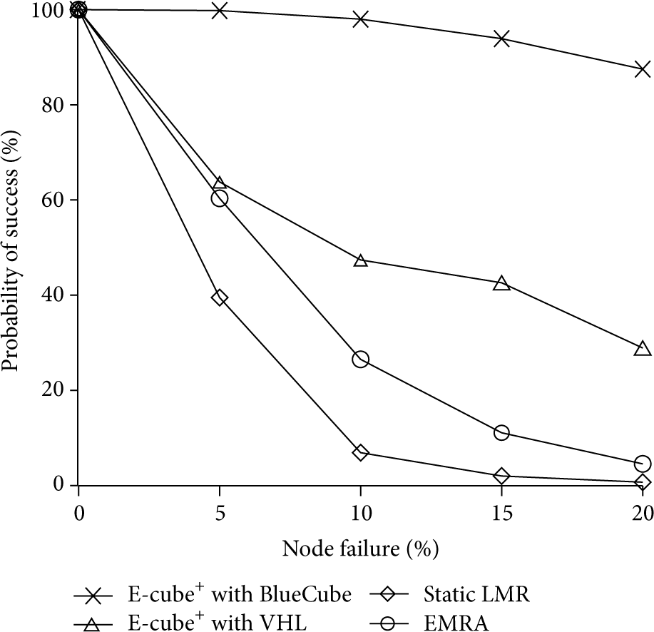
Probability of successful transmission versus percentage of node failures.

In E-cube⁺ with VHL, since the network topology is a grid, every node can connect to a maximum of four neighboring nodes, which is the same as that in the LMR. Due to routing method employed in E-cube⁺, every node has a backup route, like in a tree structure. Therefore, instead of just one backup path, multiple backup paths can be found. But in the LMR, only the source node has a single backup path. Thus, when any nodes in the main and backup paths fail, the data is not transmitted to the destination. As for EMRA, its probability of success is higher than LMR due to disjoint multiple path property.

Following the experiment with the longest pair of nodes, we tested the transmission success rate of node pairs with different Euclidean distances in a network with 10% failed nodes. In the 16 × 16 grid environment, the source node places in (0,0), and the 7 different sink locations ( $D_{i}$ ) are as following: $D_{0}$ in (2,2), $D_{1}$ in (4,4), $D_{2}$ in (6,6), $D_{3}$ in (8,8), $D_{4}$ in (11,11), $D_{5}$ in (13,13), and $D_{6}$ in (15,15). In Figure 5, it can be seen that, due to its ideal assumption, E-cube⁺ with BlueCube is able to maintain a success rate higher than 98% irrespective of the distance. E-cube⁺ with VHL, EMRA and LMR show little difference when the distance is short, as the number of possible backup nodes is limited. When the distance gradually increases, the number of nodes on the paths also increases. On the other hand, the probability of node failure also increases. However, as E-cube⁺ can acquire multiple paths, its failure rate does not increase as rapidly as that of the EMRA and LMR. Therefore, it can be seen that E-cube⁺ is always able to exhibit good fault-tolerance capability.

Figure 5

Probability of successful transmission for varying distances.

When using the E-cube⁺ method, no routing table is required and simple calculations can provide routing decisions. In order to demonstrate that E-cube⁺ does not sacrifice transmission time for saving memory space, it can be seen in Figure 6 that the 7 different distances ( $D_{0}$ to $D_{6}$ ) were used in the experiment to obtain different packet delays. From the figure, it can be seen that the routing of the static LMR through table lookup is more time-consuming than E-cube⁺ with VHL and E-cube⁺ with BlueCube. As the distance increases, when compared with the table lookups, E-cube⁺ with VHL and E-cube⁺ with BlueCube have a lesser increase in the delay, which demonstrates the simplicity of the E-cube⁺ routing method. Please note that EMRA and E-cube⁺ with BlueCube have the best performance with the lowest delay time. E-cube⁺ with BlueCube is under the assumption of strong transmission range that can make the labeled network be mapped to a k-cube topology (such as 8-cube of 256 nodes) as well as adopting E-cube⁺ routing algorithm.

Figure 6

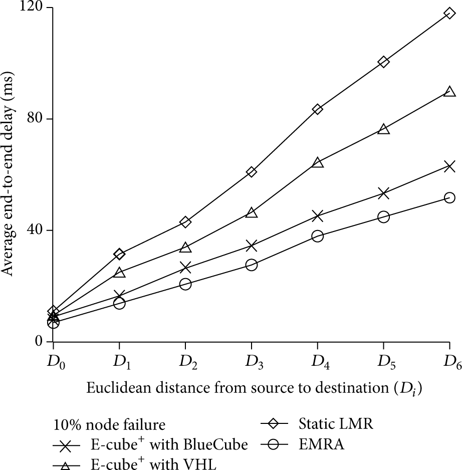
Average end-to-end delay for varying distances.

5. Conclusion

Due to the resource constraints and the existence of wireless features, wireless sensor networks are susceptible to relatively high fault rates. When certain nodes in a wireless sensor network fail, wireless network transmission will be interrupted, thus greatly lowering the reliability of the entire network. In this paper, we proposed a fault-tolerant tableless routing protocol termed E-cube⁺, to achieve a highly fault-tolerant protocol for a wireless sensor network. With these desired fault-tolerant salient features (including no routing table lookup, failure recovery guarantees, and bounded latency), E-cube⁺ is expected to become the fundamental support for wireless sensor networks.

Footnotes

Conflict of Interests

The authors declare that there is no conflict of interests regarding the publication of this paper.

References

Araujo

Mazo

Anta

Tabuada

Johansson

K. H.

System architectures, protocols and algorithms for aperiodic wireless control systems

IEEE Transactions on Industrial Informatics 2014 10 1 175 184

10.1109/TII.2013.2262281

2-s2.0-84890902858

Salman

Ghogho

Kemp

A. H.

Optimized low complexity sensor node positioning in wireless sensor networks

IEEE Sensors Journal 2014 14 1 39 46

10.1109/JSEN.2013.2278864

2-s2.0-84887860613

Huang

Energy-aware geographic routing in wireless sensor networks with anchor nodes

International Journal of Communication Systems 2013 26 1 100 113

2-s2.0-84871620318

10.1002/dac.1335

Cheng

B. C.

Liao

G. T.

Tseng

R. Y.

Hsu

P. H.

Network lifetime bounds for hierarchical wireless sensor networks in the presence of energy constraints

Computer Networks 2012 56 2 820 831

10.1016/j.comnet.2011.10.019

2-s2.0-84856026889

Dally

W. J.

Seitz

C. L.

Deadlock-free message routing in multiprocessor interconnection networks

IEEE Transactions on Computers 1987 36 5 547 553

10.1109/TC.1987.1676939

2-s2.0-0023346637

Draper

J. T.

Ghosh

Multipath E-cube algorithms (MECA) for adaptive wormhole routing and broadcasting in k-ary n-cubes

Proceedings of the 6th International Parallel Processing Symposium

March 1992

Beverly Hills, Calif, USA

407 410

2-s2.0-0026962462

Chuang

P.-J.

B.-Y.

Chao

T.-H.

Hypercube-based data gathering in wireless sensor networks

Journal of Information Science and Engineering 2007 23 4 1155 1170

2-s2.0-34547471965

Huo

Shen

Zhang

Virtual hypercube routing in wireless sensor networks for health care systems

Proceedings of the 1st International Conference on Future Information Networks (ICFIN '09)

October 2009

178 183

2-s2.0-72049085582

10.1109/ICFIN.2009.5339574

Aumann

Bender

M. A.

Fault-tolerant data structures

Proceedings of the 37th Annual Symposium on the Foundations of Computer Science (FOCS '96)

October 1996

580 589

10.

Wang

Liu

Sun

Liu

Zhou

Fault tolerance on improved distributed spanning tree structure

Proceedings of the IEEE International Conference on Advanced Computer Control (ICACC '10)

March 2010

296 300

10.1109/ICACC.2010.5487249

2-s2.0-77957964698

11.

Lin

Xia

Yao

Zhang

Liu

Dynamical jumping real-time fault-tolerant routing protocol for wireless sensor networks

Sensors 2010 10 3 2416 2437

10.3390/s100302416

2-s2.0-77955506312

12.

Che-Aron

Al-Khateeb

W. F. M.

Anwar

An enhancement of fault-tolerant routing protocol for wireless sensor network

Proceedings of the International Conference on Computer and Communication Engineering (ICCCE '10)

May 2010

Kuala Lumpur, Malaysia

10.1109/ICCCE.2010.5556790

2-s2.0-77957775539

13.

Khan

A. U. R.

Madani

S. A.

Hayat

Khan

S. U.

Clustering-based power-controlled routing for mobile wireless sensor networks

International Journal of Communication Systems 2012 25 4 529 542

10.1002/dac.1280

2-s2.0-84859157992

14.

Russell

Littman

M. L.

Trappe

Integrating machine learning in ad hoc routing: a wireless adaptive routing protocol

International Journal of Communication Systems 2011 24 7 950 966

10.1002/dac.1202

2-s2.0-79959759043

15.

Gaughan

P. T.

Yalamanchili

Adaptive routing protocols for hypercube interconnection networks

Computer 1993 26 5 12 23

10.1109/2.211888

16.

Chen

M. S.

Shin

K. G.

Adaptive fault-tolerant routing in hypercube multicomputers

IEEE Transactions on Computers 1990 39 12 1406 1416

2-s2.0-0025682423

MR1081843

10.1109/12.61061

17.

Adaptive fault-tolerant routing in cube-based multicomputers using safety vectors

IEEE Transactions on Parallel and Distributed Systems 1998 9 4 321 334

10.1109/71.667894

2-s2.0-0032049035

18.

Hoffmann

Borchert

Dietrich

Schirmeier

Kapitza

Spinczyk

Lohmann

Effectiveness of fault detection mechanisms in static and dynamic operating system designs

Proceedings of the 17th IEEE International Symposium on Object-Oriented Real-Time Distributed Computing (ISORC '14)

June 2014

Reno, Nev, USA

19.

Arun Kumar

Tagore

M. R. N.

Giri Babu Kande

D. R.

An efficient fault detection system with difference-set codes for memory applications

Proceedings of the 29th International Conference on Recent Trends in Science and Technology (RTET '13)

September 2013

43 48

20.

Cinque

Di Martino

Testa

Analyzing and modeling the failure behavior of wireless sensor networks software under errors

Proceedings of the 8th IEEE International Wireless Communications and Mobile Computing Conference (IWCMC '12)

August 2012

Limassol, Cyprus

1136 1141

10.1109/IWCMC.2012.6314366

2-s2.0-84869186112

21.

Ferguson

Noorani

A study of self-propagating mal-packets in sensor networks: attacks and defenses

Computers and Security 2011 30 1 13 27

10.1016/j.cose.2010.10.002

2-s2.0-79251600457

22.

Kumar

Sultan

Nagaraja

Chakradhar

Srivastava

Handling memory corruption faults in sensor networks

NESL Technical Report 2005 TR-UCLA-NESL-200510-04 http://nesl.ee.ucla.edu/document/show/194

23.

Intanagonwiwat

Govindan

Estrin

Heidemann

Silva

Directed diffusion for wireless sensor networking

IEEE/ACM Transactions on Networking 2003 11 1 2 16

10.1109/TNET.2002.808417

2-s2.0-0037295692

24.

Perkins

Belding-Royer

Das

Ad Hoc on-Demand Distance Vector (AODV) Routing 2003 3561

RFC

25.

Johnson

D. B.

Maltz

D. A.

Dynamic source routing in Ad Hoc wireless networks

Mobile Computing 1996 353 153 181 The Kluwer International Series in Engineering and Computer Science

26.

Huang

Load-balanced and link-disjoint multipath routing for wireless sensor networks

Advances in Electrical Engineering and Electrical Machines 2011 134 395 403 Lecture Notes in Electrical Engineering

10.1007/978-3-642-25905-0_52

27.

Jung

S.-R.

Lee

J.-H.

Roh

B.-H.

An optimized node-disjoint multi-path routing protocol for multimedia data transmission over wireless sensor networks

Proceedings of the International Symposium on Parallel and Distributed Processing with Applications (ISPA '08)

December 2008

Seoul, Republic of Korea

958 963

10.1109/ISPA.2008.64

2-s2.0-60649103992

28.

Ganesan

Govindan

Shenker

Estrin

Highly-resilient, energy-efficient multipath routing in wireless sensor networks

ACM SIGMOBILE Mobile Computing and Communications Review 2001 5 4 11 25

10.1145/509506.509514

29.

Key

Massoulié

Towsley

Path selection and multipath congestion control

Proceedings of the 26th IEEE International Conference on Computer Communications (IEEE INFOCOM '07)

May 2007

Anchorage, AK, USA

143 151

10.1109/INFCOM.2007.25

2-s2.0-34548324845

30.

Shi

Cai

Wei

Shan

An energy-adaptive multiple paths routing approach for wireless sensor networks

Journal of Mobile Multimedia 2012 8 1 34 48

2-s2.0-84860857308

31.

Marina

M. K.

Das

S. R.

On-demand multipath distance vector routing in ad hoc networks

Proceedings of the 9th International Conference on Network Protocols

November 2001

Riverside, Calif, USA

14 23

2-s2.0-0035703920

32.

Joseph

L. N.

Uma

G. V.

Reliability based routing in wireless sensor networks

International Journal of Computer Science and Network Security 2006 6 12 331 338

33.

Kim

Fonseca

Culler

Reliable transfer on wireless sensor networks

Proceedings of the 1st Annual IEEE Communications Society Conference on Sensor and Ad Hoc Communications and Networks (IEEE SECON '04)

October 2004

449 459

34.

Chang

C.-T.

Chang

C.-Y.

Sheu

J.-P.

BlueCube: constructing a hypercube parallel computing and communication environment over Bluetooth radio systems

Journal of Parallel and Distributed Computing 2006 66 10 1243 1258

10.1016/j.jpdc.2006.04.018

2-s2.0-33748058855

35.

Hou

Tipper

Kabara

Label-based multipath routing (LMR) in wireless sensor networks

Proceedings of the 6th International Symposium on Advanced Radio Technologies (ISART '04)

2004

36.

Intanagonwiwat

Govindan

Estrin

Directed diffusion: A scalable and robust communication paradigm for sensor networks

Proceedings of the 6th Annual International Conference on Mobile Computing and Networking (MOBICOM '00)

August 2000

Boston, Mass, USA

56 67

2-s2.0-0034539015

37.

Toce

Mowshowitz

Stone

Dantressangle

Bent

HyperD: a hypercube topology for dynamic distributed federated databases

Annual Conference of the International Technology Alliance

September 2011

Adelphi, Md, USA

E-Cube + Routing Protocol for Wireless Sensor Networks in the Presence of Network Failures

Abstract

1. Introduction

2. Related Work

3. Fault-Tolerant E-Cube+ Routing

3.1. Packet Header Format

3.2. Routing Algorithm

Algorithm 1: The E-cube+ routing algorithm.

3.3. Example

Case 1 (normal routing with no failure nodes).

Case 2 (backup routing with a single failure node).

Case 3 (backward routing during multiple failures).

3.4. Property

Theorem 1.

Proof.

Theorem 2.

Proof.

3.5. Topology Control Concept Illustration

4. Simulation and Results

5. Conclusion

Footnotes

Conflict of Interests

References

3. Fault-Tolerant E-Cube⁺ Routing

Algorithm 1: The E-cube⁺ routing algorithm.