ECAPM: An Enhanced Coverage Algorithm in Wireless Sensor Network Based on Probability Model

Abstract

How to cover a monitored area with the minimum number of sensor nodes is a fundamental in wireless sensor network (WSN). To address this problem, this paper proposes ECAPM, that is, Enhanced Coverage Algorithm Based on Probability Model. Given an area to monitor, ECAPM can calculate the minimum number of sensor nodes to cover that area. Firstly, ECAPM introduces the method to compute the expectation of probability that a sensor node is covered. Then ECAPM presents the procedure of expected value calculation when target node is covered by one sensor node and N sensor nodes. Finally ECAPM verifies the relation of proportional function when random variables are not independent. The simulation results show that ECAPM can cover the monitored area effectively with less sensor nodes and improve the quality of coverage.

1. Introduction

Wireless sensor network is a wireless network that combines integrated sensor technology, micro- and special electromechanical technology, and wireless communication technology. It transmits data by a great quantity of sensor nodes through the form of self-organization and multihop mode [1, 2]. Sensor nodes are characterized by small volume, limited energy, the ability of perception, calculation, and communication. It can be widely used in the fields of national defense, military, transportation, health care, environment monitoring, antiseismic work, disaster relief, and so on [3, 4]. At present, there are two types of deployment scenarios of the sensor nodes, namely, manual deployment and random deployment. The use of manual deployment is limited to certain environment. Under extreme circumstances, random placement is more preferred [5–7]. Random placement does not need to take environmental factors into account. Under very bad environment, aircraft random placement mechanism is often used to deploy the sensor nodes. Although the damage of human activity can be reduced in the random placement, there exist several shortcomings. Due to random deployment [8, 9], certain scope in the monitored area will be in high-density centralized state, which will cause a series of problems to network expanding ability, comprehensive serving ability, data communication, signal interference, and energy saving [10, 11].

Target nodes are covered effectively under satisfying certain coverage probability, but there exist some drawbacks, which are mainly reflected in the following respects. Firstly, although data fusion is finished and target nodes are effectively covered, the energy consumption of the sensor nodes is not taken into account. Secondly, it needs a pointing device to obtain the position of sensor nodes, such as GPRS, which increases the cost of network system operations virtually, and adds the disturbance between signals as well [12, 13]. Because of the disturbance between signals, covering relationships of the sensor nodes cannot be figured out accurately. Thirdly, network model is too ideal and it is difficult to achieve the desired result. Fourthly, the algorithm needs much more complicated calculation [14, 15].

Based on these problems, the basic problem is how to give effective cover for domain in the monitored area, how to reduce consume of sensor nodes’ energy, and how to effectively cover the maximum area or the major destination node by fewest sensor nodes. Building on the premise of some certain coverage, we do not require the complete cover of sensor node in the monitored area, we hope just to keep some coverage to the monitored area. Therefore, to some extent, coverage rate is one of the standards measuring quality of network service.

2. Related Works

In recent years, many experts at home and abroad have analyzed and discussed the features of wireless sensor network elaborately and profoundly. Literature [16] proposed arithmetic to maintain connected coverage. This arithmetic makes use of relative adjacency graph and deployment features of node to offer sensor node maintaining network unicom and coverage in the process of mobile deployment. This arithmetic all keeps the network connectivity by the network topology formed by sensor node moving in any direction. The coverage feature of mobile target node depends on constraints of network connectivity. Literature [17] proposed centralized cluster K cover configuration protocol. This protocol analyses the coverage protocol by making use of the construction network model and gives four kinds of K cover configuration protocols; they are centralized randomized connected K coverage (CERACCk); T-clustered randomized connected K coverage (T-CRACCk); D-clustered randomized connected K coverage (D-CRACCk), and distributed randomized connected K coverage (DIRACCk). This literature proves that when $K\ge 3$ , it needs k sensor nodes when the Lu Luo triangle side which is formed by network model after coverage is the perceived radius of the nodes and it gives the comparison of communication radius and perceived radius after completing the K coverage. At the same time, it gives the counting process of the fewest sensor node quantities in the completed coverage area and the computational formula of the need of sensor node density in the monitored area. Literature [18] proposed arithmetic of K degree discrete barrier coverage for maximizing the network lifetime. The algorithm from the theoretical perspective analyses the network model coverage higher limit and the lower limit of the condition of the existence of specific barriers; let all target nodes concerned complete effectively covering; in network energy consumption gives a sensor node scheduling algorithm, which brings in a greedy algorithm to redeployment the sensor node, using scheduling mechanism between sensor nodes to complete the state transitions between the sensor nodes and ultimately achieving the purpose of maximizing the network lifecycle. Reference [19] by mixed integer programming approach presents heuristic algorithm coverage. The algorithm studies the sensor nodes set intersect and sensor nodes perception radius adjustable heuristic coverage. In order to further improve the literature [19] algorithm, Yang et al. [20] take approximately the coverage area of the target node in the literature [19] as the monitoring area and use high-density deployment of sensor nodes to build a collection of complete coverage connectivity coverage of the target coverage area. In these two studies based on the literature, Liu et al. [21] do a lot of research work of the target coverage problem in the condition of defining a sensor node which can only cover a target node, giving out the target solving process node coverage at any given moment. Reference [22] through artificial bee colony algorithm and particle swarm optimizes scheduling problems for the sensor nodes by heuristic configuring methods to identify the optimal deployment path, giving the position after the best deployment of sensor nodes and theoretical calculations calculation of the lifetime limit network. Reference [23] proposed an energy efficient routing algorithm maintaining connectivity coverage, an Energy-Efficient Coverage and Connectivity Preserving Routing Algorithm (ECCRA), the algorithm uses the network model to construct double coverage area, the expected value of the final upper limit is determined on completion of the monitoring area covered, and the effective coverage of at least knowledge of sensor nodes calculated probability covered by probability value and the number of coverage desired values. References [22, 23], to some extent, have completed the monitoring area effective coverage and suppressed rapid energy consumption of sensor nodes, but the calculation of the two algorithms is large, owning a high complexity of the algorithm, and the nodes of the monitoring area covered a longer time to complete. Reference [24] proposed a self-organizing overlay control protocol (SOCCP: Self-Organized Coverage and Connectivity Protocol). The agreement by calculating the location information located in the monitoring area of the sensor nodes and a subset of nodes determines the coverage area of coverage and the completion of the conversion node status by scheduling mechanism of nodes. Reference [25] proposed the algorithm calculating the sensor nodes within the network coverage of the value of the two cases and boundary coverage connectivity algorithm (Square Coverage and Connectivity Probability (SCCP) Model) under a basic probability model and then get the node within the monitoring area of the network coverage area of the total expected value. Literature [26] proposed a rule based on the linear energy efficient multiobjective coverage algorithm (Energy-Efficient Target Coverage Algorithm (ETCA)). The algorithm uses the cluster architecture to solve the problem of multiobjective coverage through coverage and the residual energy of the sensor calculation to give a linear manner optimal coverage for multiple target nodes. Reference [27] gives the coverage based on energy-efficient multiobjective algorithm optimization by means of integer linear programming and for minimizing node deployment of costs and energy consumption.

In order to study the coverage problem better in wireless sensor networks, the area of coverage model to was monitored study the target node, the probability of covering the sensor nodes of the target node is 1, and the probability uncovered 0. Therefore, we propose Enhanced Coverage Algorithm Based on Probability Model (ECAPM). The algorithm is studied in the following four areas.

• (1)

Conduct a study of the relevant literature; point out the advantages and disadvantages of various cover algorithms; this paper describes ECAPM's central idea and builds a network covering the system model.

(2)

Use of network coverage system model incorporates the characteristics of normal distribution random deployment of node; the mobile target node through the fan-shaped area formed by the sensor of sensor nodes gives out the coverage and coverage quality of the monitoring area of the n sensor nodes and the expected value of the solution process.

(3)

The entire network system model is calculated; set the random variable X in the monitoring area (in square area for the study), the first time when the sensor nodes and the expected value and the variance of the certification process is completed after the expected value of N times covering solving process, simultaneously monitor the implementation of the entire area covered by the minimum effective amount of sensor nodes solving process.

(4)

By simulating, verify the algorithm of its effectively cover in the article ECAPM monitoring in different regions, and situation of comparison of coverage between the operation of the sensor nodes and the number of different parameters.

3. System Model and the Analysis of Coverage Quality

The proposed algorithm is based on the following four assumptions.

• (1)

At original time, communications ranges and perception ranges of each sensor node in the wireless sensor network are disc-shaped and remain still.

(2)

Each sensor node can obtain the location of itself by GPS.

(3)

All sensor nodes are deployed in a square region at random conforming to normal distribution, regardless of the condition of the border existence.

(4)

At original time, the energy of each sensor node is equal, so is their respective status.

3.1. Basic Definition

Definition 1 (cover set).

Target set is T, arbitrary target node $t_k$ is given, and $t_k\in T$ . In a certain time interval, if there had at least one target node in the target set covered by the any arbitrary sensor node in the sensor node set, it is called that target node $t_k$ is covered by the sensor node $s_j$ and the set formed by the $t_k$ is called cover set.

Definition 2 (cover association).

Any two sensor nodes $s_i$ , $s_j$ are given and the covered area by them in the monitored area is $A(s_i)$ , $A(s_j)$ separately, $A(s_i)\cap A(s_j)\ne Ф$ , and it is called cover associated with one another.

Definition 3 (coverage fraction).

The coverage fraction of the working sensor node $s_j$ randomly deployed in the monitored area Ω is

$$\begin{array}{cc}& P\left(S,\Omega \right)=\frac{\sum A\left(s_i\right)}{A\left(\Omega \right)},\end{array}$$

(1)

where S is the sensor node set, $A(s_i)$ is the cover area of the sensor node I, and $A(\Omega )$ is the monitored area.

3.2. System Model

To research problem easily, square, three sensor nodes and the movement of the target nodes are regarded as research subjects in the paper, shown in Figure 1.

Figure 1

Covers schematic of associated property.

In Figure 1, $s_1$ , $s_2$ , and $s_3$ are the sensor nodes and dotted lines are the track that the target nodes are walking on. As we can see from Figure 1, the movement of the target nodes and three circles intersect, forming three sectors by connecting intersection. Sector $A{s}_{1}B$ belongs to $s_1$ , sector $B{s}_{2}C$ belongs to $s_2$ , sector $C{s}_{3}D$ belongs to $s_3$ , and the sector area can be resolved based on the geometry theory; namely,

$$\begin{array}{cc}& {\displaystyle \bigcup }\left(S_s\right)=\frac{{\alpha }_i\pi }{\mathrm{360}}{r}^{\mathrm{2}}={\phi }_i\pi r^{\mathrm{2}}.\end{array}$$

(2)

Taking $s_1$ as examples, $S_s$ is the sector area and ${\theta }_i$ is central angle. If it is expressed in radians, set ${\phi }_i={\alpha }_i/\mathrm{360}$ and r is the perceived radius. To the movement of target nodes, curve equation is proposed by means of data fitting:

$$\begin{array}{cc}& f\left(x\right)=b_n{x}^n+b_{n-\mathrm{1}}{x}^{n-\mathrm{1}}+\cdots b_{\mathrm{0}},\end{array}$$

(3)

where $b_i$ is the proportion dimension and $f(x)$ is the data fitting equation.

3.3. Analysis of the Coverage Quality

This section discusses the coverage fraction of the sensor nodes, the solving process of expected values of the cover quality of n sensor nodes in the monitored area, the normalized model of expected values and variance, and validation process of the number of the least sensor nodes in the covered monitored area.

Theorem 4.

Supposing that the coverage fraction of the sensor nodes in the monitored area is $P(A)$ , the coverage fraction of point i in the monitored area is $P\left(nA\right)=\mathrm{1}-{\prod }_{\mathrm{1}\le i\le n}\left(\mathrm{1}-P\left(A\right)\right)$ .

Proof.

It is proved by mathematical induction. When sensor nodes are working, each sensor node in the covered area is independent of one another. Hence, the probability that two sensor nodes are working is

$$\begin{array}{l}P\left(A+A\right)=P\left(A\right)+P\left(A\right)-P\left(A\right)P\left(A\right)=\mathrm{2}p-p^{\mathrm{2}}\\ =\mathrm{1}-{\left(\mathrm{1}-p\right)}^{\mathrm{2}}.\end{array}$$

(4)

The probability that three sensor nodes are working is

$$\begin{array}{l}P\left(A+A+A\right)=P\left(A+A\right)+P\left(A\right)\\ -P\left(A+A\right)P\left(A\right).\end{array}$$

(5)

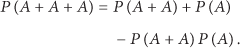
Putting formulas (4) and (5) together, we have

$$\begin{array}{cc}& P\left(A+A+A\right)=\mathrm{1}-{\left(\mathrm{1}-p\right)}^{\mathrm{3}}.\end{array}$$

(6)

When $i=n$ , namely, $P\left(nA\right)=P\left[\left(n-\mathrm{1}\right)A\right]+P\left(A\right)-P\left[\left(n-\mathrm{1}\right)A\right]P\left(A\right)$ is established; when I is equal to $n+1$ , put it into the left formula, and then

$$\begin{array}{cc}& P\left(nA\right)=\mathrm{1}-{\displaystyle \prod }_{\mathrm{1}\le i\le n}\left(\mathrm{1}-P\left(A\right)\right).\end{array}$$

(7)

It has been proved.

Corollary 5.

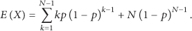
Supposing that the coverage fraction of the sensor nodes in the covered area is P, when N times coverage is finished, expected values of the sensor nodes are $E(X)=\left[1-{\left(1-p\right)}^N\right]p^{-1}$ .

Proof.

Setting x equal to transfer number when target node is covered for the first time, then the possible value of X is $X\in [\mathrm{1,2},3,\dots ,N]$ . When $X=k$ and $1\le k\le N-1$ , it shows that target node is not covered for the first $N-1$ times, so the distributed density function of x is

$$\begin{array}{cc}& P\left(X=k\right)=\left\{\begin{array}{cc}p{\left(\mathrm{1}-p\right)}^{k-\mathrm{1}},\hfill & k=\mathrm{1,2},\mathrm{3},\dots ,N-\mathrm{1},\hfill \\ {\left(\mathrm{1}-p\right)}^{N-\mathrm{1}},\hfill & k=N.\hfill \end{array}\right.\end{array}$$

(8)

Then,

$$\begin{array}{cc}& E\left(X\right)={\displaystyle \sum }_{k=\mathrm{1}}^{N-\mathrm{1}}kp{\left(\mathrm{1}-p\right)}^{k-\mathrm{1}}+N{\left(\mathrm{1}-p\right)}^{N-\mathrm{1}}.\end{array}$$

(9)

If set $q=1-p$ and $S={\sum }_{k=\mathrm{1}}^{N-\mathrm{1}}k{\left(\mathrm{1}-p\right)}^{k-\mathrm{1}}$ , then $S={\sum }_{k=\mathrm{1}}^{N-\mathrm{1}}k{q}^{k-\mathrm{1}}$ , and the left and right of the equation are multiplied by q; then $qS={\sum }_{k=\mathrm{1}}^{N-\mathrm{1}}k{q}^k$ ; namely,

$$\begin{array}{l}S=\frac{\mathrm{1}-q^{N-\mathrm{1}}}{{\left(\mathrm{1}-q\right)}^{\mathrm{2}}}-\frac{\left(N-\mathrm{1}\right)q^{N-\mathrm{1}}}{\mathrm{1}-q}\\ =\frac{\mathrm{1}-{\left(\mathrm{1}-p\right)}^{N-\mathrm{1}}}{p^{\mathrm{2}}}-\frac{\left(N-\mathrm{1}\right){\left(\mathrm{1}-p\right)}^{N-\mathrm{1}}}{p}.\end{array}$$

(10)

Putting S into formula (9), we have

$$\begin{array}{l}E\left(X\right)=p\left(\frac{\mathrm{1}-{\left(\mathrm{1}-p\right)}^{N-\mathrm{1}}}{p^{\mathrm{2}}}-\frac{\left(N-\mathrm{1}\right){\left(\mathrm{1}-p\right)}^{N-\mathrm{1}}}{p}\right)\\ +N{\left(\mathrm{1}-p\right)}^{N-\mathrm{1}}\\ =\frac{\mathrm{1}-{\left(\mathrm{1}-p\right)}^{N-\mathrm{1}}}{p}-\left(N-\mathrm{1}\right){\left(\mathrm{1}-p\right)}^{N-\mathrm{1}}\\ +N{\left(\mathrm{1}-p\right)}^{N-\mathrm{1}}\\ =\frac{\mathrm{1}-{\left(\mathrm{1}-p\right)}^{N-\mathrm{1}}+p{\left(\mathrm{1}-p\right)}^{N-\mathrm{1}}}{p}\\ =\left[\mathrm{1}-{\left(\mathrm{1}-p\right)}^N\right]p^{-\mathrm{1}}.\end{array}$$

(11)

It has been proved.

Corollary 6.

Setting that the coverage fraction of the sensor node is P, when moving target nodes are covered by the sensor node set for the first time, the expected value is $E(X)=1/p$ , and variance is $D(X)=1-p/p^2$ .

Proof.

In the monitored area, the probability of coverage by arbitrary sensor node is p, and then the probability that it is not covered is $1-p$ . Setting $q=1-p$ , supposing that sensor node k covers moving target node for the first time, then

$$\begin{array}{l}E\left(X\right)={\displaystyle \sum }_{k=\mathrm{1}}^{N}kp{q}^{k-\mathrm{1}}=p{\left({\displaystyle \sum }_{k=\mathrm{1}}^N{q}^k\right)}^{\prime }=p{\left(\frac{q}{\mathrm{1}-q}\right)}^{\prime }\\ =\frac{\mathrm{1}}{p},\\ E\left(X^2\right)={\displaystyle \sum }_{k=1}^N{k}^{2}p{q}^{k-1}=pq{\displaystyle \sum }_{k=1}^{N}k\left(k-1\right)q^{k-2}+\frac{1}{p}\\ =pq{\left({\displaystyle \sum }_{k=1}^N{q}^k\right)}^{\prime \prime }+\frac{1}{p}=\frac{1+q}{p^2},\\ D\left(X\right)=E\left(X^{\mathrm{2}}\right)-E\left(X\right)=\frac{\mathrm{1}-p}{p^{\mathrm{2}}}.\end{array}$$

(12)

The theorem is proved.

Theorem 4 and Corollaries 5 and 6 provide the calculating process that sensor node covers moving target nodes. In general, the movement of moving target nodes and area covered by the sensor nodes appear sector state. How to calculate the expected value of sensor nodes in the fan-shaped and square monitored area and the number of nodes in the covered monitored area is shown here. Based on the probability theory, according to perceived radius of sensor nodes, the formed coverage angle and theoretical knowledge in geometry, we calculate the expected value of the sensor node.

Definition 7 (effective coverage).

Based on Definition 1, if all the target nodes in certain monitored area are covered by the sensor node set, it is called the effective coverage of the sensor nodes. The area that is covered by sensor nodes is called effective covered area.

Definition 8 (node redundancy).

To the sensor node set, the ratio of the monitored area of the adjacent node perceived by any sensor node and the overlapped area forming from multicoverage to the monitored area is called redundancy; namely,

$$\begin{array}{cc}& \psi \left(i\right)=\frac{S\left({{\displaystyle \bigcup }}_{\left(\left(i,j\le N\right)\cup \left(i\cap j\right)\right)}{s}_i\right)}{S\left(\Omega \right)}.\end{array}$$

(13)

Theorem 9.

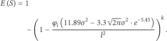
In the monitored area Ω, the expected value of the coverage quality of k working sensor nodes is

$$\begin{array}{l}E\left(S\right)=\mathrm{1}\\ -{\left(\mathrm{1}-\frac{{\phi }_i\left(\mathrm{11.89}{\sigma }^{\mathrm{2}}-\mathrm{3.3}\sqrt{\mathrm{2}\pi }{\sigma }^{\mathrm{2}}·e^{-\mathrm{5.45}}\right)}{l^{\mathrm{2}}}\right)}^k.\end{array}$$

(14)

Proof.

Regarding Figure 1 as research object and supposing that there are k working sensor nodes in the square monitored area. To the sector formed from the lines between the intersections between the moving track and k working sensor nodes and the center, according to the calculating method of coverage fraction in the formula (1), coverage fraction of any target node that is covered by the shadows is

$$\begin{array}{cc}& P_t=\frac{{\displaystyle \bigcup }\left(S_s\right)}{S\left(\Omega \right)}=\frac{{\phi }_i\pi r^{\mathrm{2}}}{l^{\mathrm{2}}},\end{array}$$

(15)

where ${\phi }_i={\sum }_{i=\mathrm{1}}^N{\alpha }_i$ .

All the sensor nodes in the sensor node set obey normal distribution $N(r_0,{\sigma }^2)$ , where $r_0$ is the average of the perceived radius of the sensor nodes, ${\sigma }^2$ is the variance of the perceived radius, and $r_0\ge 3.3\sigma$ . According to [21], the coverage fraction of any point in the monitored area is

$$\begin{array}{cc}& P_i={{\displaystyle \int }}_{\mathrm{0}}^{\mathrm{2}{r}_{\mathrm{0}}}\frac{{\phi }_i\pi r^{\mathrm{2}}}{\sqrt{\mathrm{2}\pi }\sigma l^{\mathrm{2}}}·e^{-\left({\left(r-r_{\mathrm{0}}\right)}^{\mathrm{2}}/\mathrm{2}{\sigma }^{\mathrm{2}}\right)}dr.\end{array}$$

(16)

Set $x=(r-r_{\mathrm{0}})/\sigma$ and put it into formula (16); then

$$\begin{array}{l}{P}_i=\frac{{\phi }_i\pi }{\sqrt{2\pi }\sigma l^2}{\int }_{-(r_0/\sigma )}^{r_0/\sigma }\sigma {(x\sigma +r_0)}^2\cdot e^{-(x^2/2)}dx\hfill \\ \hspace{0.17em}\hspace{0.17em}\hspace{0.17em}\hspace{0.17em}\hspace{0.17em}=\frac{{\phi }_i\pi }{\sqrt{2\pi }{l}^2}\left({\int }_{-(r_0/\sigma )}^{r_0/\sigma }\left(x^2{\sigma }^2+2x\sigma r_0+r_0^2\right)\cdot e^{-(x^2/2)}\right)dx\hfill \\ \hspace{0.17em}\hspace{0.17em}\hspace{0.17em}\hspace{0.17em}\hspace{0.17em}=\frac{{\phi }_i\pi }{\sqrt{2\pi }{l}^2}({\int }_{-(r_0/\sigma )}^{r_0/\sigma }-x{\sigma }^2\left(e^{-(x^2/2)}\right)\hfill \\ \hspace{0.17em}\hspace{0.17em}\hspace{0.17em}\hspace{0.17em}\hspace{0.17em}+r_0^2{\int }_{-(r_0/\sigma )}^{r_0/\sigma }{e}^{-(x^2/2)}dx)\hfill \\ \hspace{0.17em}\hspace{0.17em}\hspace{0.17em}\hspace{0.17em}\hspace{0.17em}=\frac{{\phi }_i\pi }{\sqrt{2\pi }{l}^2}({-x{\sigma }^2\cdot e^{-(x^2/2)}|}_{-(r_0/\sigma )}^{r_0/\sigma }+\sqrt{2\pi }{\sigma }^2\hfill \\ \hspace{0.17em}\hspace{0.17em}\hspace{0.17em}\hspace{0.17em}\hspace{0.17em}+\sqrt{2}\pi r_0^2)\hfill \\ \hspace{0.17em}\hspace{0.17em}\hspace{0.17em}\hspace{0.17em}\hspace{0.17em}=\frac{{\phi }_i\left(\pi \left(r_0^2+{\sigma }^2\right)-\sqrt{2\pi }{r}_0\sigma \cdot e^{-(r_0/2{\sigma }^2)}\right)}{l^2}.\hfill \end{array}$$

(17)

Namely,

$$\begin{array}{cc}& P_i=\frac{{\phi }_i\left(\pi \left({r_{\mathrm{0}}}^{\mathrm{2}}+{\sigma }^{\mathrm{2}}\right)-\sqrt{\mathrm{2}\pi }{r}_{\mathrm{0}}\sigma ·e^{-\left(r_{\mathrm{0}}/\mathrm{2}{\sigma }^{\mathrm{2}}\right)}\right)}{l^{\mathrm{2}}}.\end{array}$$

(18)

If set P meets the requirement of the minimum coverage fraction, then put the minimum of $r_0$ into formula (18):

$$\begin{array}{cc}& P_i\approx \frac{{\phi }_i\left(\mathrm{11.89}\pi {\sigma }^{\mathrm{2}}-\mathrm{3.3}\sqrt{\mathrm{2}\pi }{\sigma }^{\mathrm{2}}·e^{-\mathrm{5.45}}\right)}{l^{\mathrm{2}}}.\end{array}$$

(19)

Formula (19) provides the coverage fraction of some sensor node for the monitored area. According to the proof of Theorem 4, when k sensor nodes are working, the expected value of the coverage fraction is

$$\begin{array}{l}E\left(S\right)=\mathrm{1}\\ -{\left(\mathrm{1}-\frac{{\phi }_i\left(\mathrm{11.89}{\sigma }^{\mathrm{2}}-\mathrm{3.3}\sqrt{\mathrm{2}\pi }{\sigma }^{\mathrm{2}}·e^{-\mathrm{5.45}}\right)}{l^{\mathrm{2}}}\right)}^k.\end{array}$$

(20)

The theorem is proved.

To k sensor nodes in the whole monitored area, the expected value of the coverage quality mainly depends on sector angle, variance of the normal distribution, and the monitored area.

Theorem 10.

The minimum number of nodes to cover the square monitored area is $N=\ln (\mathrm{1}-\epsilon )\ln {\left(\mathrm{1}-({\phi }_i\pi r^{\mathrm{2}}/l^{\mathrm{2}})\right)}^{-\mathrm{1}}$ .

Proof.

Very small numbers $\epsilon \hspace{0.17em}\hspace{0.17em}(\epsilon =0.00005)$ are given and the conclusion of the Theorem 4 is regarded as computed criteria. To any sensor node whose energy is not equal to zero, the coverage fraction is more than ε; namely,

$$\begin{array}{cc}& P\left(A\right)=\mathrm{1}-{\displaystyle \prod }_{\mathrm{1}\le i\le n}\left(\mathrm{1}-P\left(A\right)\right)\ge \epsilon .\end{array}$$

(21)

Then $\mathrm{1}-{\left(\mathrm{1}-p\right)}^N\ge \epsilon$ , put formula (16) into formula (21), and then

$$\begin{array}{cc}& \mathrm{1}-{\left(\mathrm{1}-\frac{{\phi }_i\pi r^{\mathrm{2}}}{l^{\mathrm{2}}}\right)}^N\ge \epsilon .\end{array}$$

(22)

After solving (22), we have

$$\begin{array}{cc}& N\le \ln \left(\mathrm{1}-\epsilon \right)\ln {\left(\mathrm{1}-\frac{{\phi }_i\pi r^{\mathrm{2}}}{l^{\mathrm{2}}}\right)}^{-\mathrm{1}}.\end{array}$$

(23)

When left and right sides of the above formula are equal, N is the number of the least sensor nodes. It has been proved.

3.4. Realization of the ECAPM Algorithm

The sensor nodes are deployed in the scope of the key target nodes by the geometric graphics theory and the target node we focus on should be guaranteed to be covered by at least one sensor node. Associated property relationships of the working sensor nodes can be found in the sensor node set [22, 23]. Number of the least covered nodes can be determined by the function relation between coverage fractions. For the ECAPM algorithm, the computation cost is lower and it is less complicated so that network quality and performance are improved (see Algorithm 1).

Algorithm 1

Input: $${\mathrm{r}}_{\mathrm{0}},\mathrm{r},{\mathrm{\sigma }}_{\max },{\mathrm{n}}_{\max },\mathrm{l}$$

Output: $${\mathrm{\sigma }}_{\text{opt}},{\mathrm{n}}_{\text{opt}}$$

Initialization: $$\mathrm{n}\leftarrow \text{null}$$ ;

(1)       Procedure

(2)     Begin

(3)     for   $$\mathrm{int}\mathrm{\sigma }=\mathrm{1}$$   to   $${\mathrm{\sigma }}_{\max }$$

(4)    for   $$\mathrm{int}n=\mathrm{1}$$   to   $${\mathrm{n}}_{\max }$$

(5)         if ( $$\text{coverage}(\sigma ,r_{\mathit{0}},r,n_{\max })\ge l$$ )

(6)           Computing probability;

(7)         then

(8)    n ← add $$(\mathrm{\sigma },{\mathrm{n}}_{\max }$$ , coverage(σ, 8

(9)         $${\mathrm{r}}_{\mathrm{0}},\mathrm{r},{\mathrm{n}}_{\max }$$ ));

(10)       end

(11)      end

(12)     end

(13)     for   $$\mathrm{int}n=\mathit{1}$$   to   $${\mathrm{n}}_{\max }$$

(14)        if (node[i] == False)

(15)            {

(16)           node[i] = $$S(i)$$ ;

(17)           Return the computing result

(18)           of (20);

(19)         Return the computing result.

(20)          of (21);

(21)             }

(22)      then

(23)           goto (3)

(24)     end

(25)   $$\text{print}f(\text{“}\mathrm{\%}\mathrm{d},\mathrm{\%}\mathrm{d}\text{”},{\mathrm{\sigma }}_{\text{opt}},{\mathrm{n}}_{\text{opt}}$$ );

(26)    end

4. Evaluations

To validate the algorithm of the paper, we use MATLAB as the simulation tool. Different network coverage scale is simulated by changing the monitored area scale; coverage quality changes in the same network coverage are proposed by use of the change of the σ value range. For different coverage quality, we propose the change curves between sensor nodes and the working nodes and so on. The parameters that are involved in the algorithm of the paper are as follows:

•  

monitored area 1: $100\mathrm{\ast }100$  m²;

 

monitored area 2: $200\mathrm{\ast }200$  m²;

 

monitored area 3: $400\mathrm{\ast }400$  m²;

 

perceived radius: 10 m;

 

sensor node energy: 5 J;

 

number of Sensor nodes: 600.

Experiment 1.

When $\sigma =1$ , three different monitored areas are effectively covered, each simulation lab result is an average of 100 times, the change curves of the sensor node number against coverage fraction is showed in Figure 2.

Figure 2

Change curves in different monitored area.

As you can see from Figure 2, it reflects the change curves of the number of the sensor nodes and the coverage probability change. As we can see from Figure 2, with the increasing of the sensor working nodes, the coverage fraction is increased. Less working sensor nodes are needed for smaller covered area. It is considered in the paper that when the coverage fraction reaches 99.9%, the monitored area is effectively covered. When $100\mathrm{\ast }100$  m² is achieved, 120 sensor working nodes are needed; when $200\mathrm{\ast }200$  m² is achieved, 204 sensor working nodes are needed; when $400\mathrm{\ast }400$  m² is achieved, 378 sensor working nodes are needed. Before the coverage fraction reaches 90%, the coverage fraction increases steadily. When the coverage fraction is between the number 90%~99.9%, it increases rapidly. The main reason is that it needs more working sensor nodes in a larger monitored area but the coverage hole number is less, so the coverage fraction increment changes rapidly; smaller monitored area needs less working sensor nodes, so the coverage fraction increment changes slowly, relative to the larger monitored area.

$400\mathrm{\ast }400$  m² as the simulation area, change curves of the coverage fraction with the number of the working sensor nodes when σ is in the different value ranges are showed in Figure 3.

Figure 3

Change curves of the coverage fraction different from σ.

Figure 3 reflects the change curves of the coverage fraction with the number of the working sensor nodes when σ is different. Because of the limit of $r_0\ge 3.3\sigma$ , $\sigma =\{\mathrm{0,1},\mathrm{2,3}\}$ in the paper. As we can see from Figure 3, when σ is equal to four different values, the coverage fraction of all presents the increasing property. When coverage fraction is equal, the less σ is, the more the working nodes are needed and vice versa. It mainly depends on the expected value of the cover quality of the monitored area in Theorem 9. To the same monitored area, the larger the expected value of the cover quality of the monitored area is, the less the nodes to achieve complete coverage are needed and the higher the speed is.

Experiment 2.

$400\hspace{0.17em}\mathrm{\ast }\hspace{0.17em}400$  m² as the monitored area, at the same σ, the comparison between the needed working nodes to meet different coverage fraction and the overall sensor node number is showed in the Figure 4.

Figure 4

(a) When $\sigma =0$ , the variation curves of the sensor node number and the working node number. (b) When $\sigma =1$ , the variation curves of the sensor node number and the working node number. (c) When $\sigma =2$ , the variation curves of the sensor node number and the working node number. (d) When $\sigma =3$ , the variation curves of the sensor node number and the working node number.

Figure 4 presents the change curves of the number of the working nodes to the number of the whole sensor nodes for four different coverage probabilities (coverage probability (CP)) in the case of the same σ. The change process of CP value from 85% to 100% when σ is equal to 0 is presented in Figure 4(a). Taking CP = 100%, for example, when CP is equal to 100%, the number of working nodes maintains 390, mainly because that to the same σ, the higher the CP is, the more the working nodes needed are, so when CP is equal to 100%, slope value of it is higher. The principle of the three other figures is similar to above processes. Four figures in the Experiment 3 can be divided into two groups: the first one is Figures 4(a) and 4(b), and the other one is Figures 4(c) and 4(d). As we can see, by comparing Figure 4(b) with Figure 4(c), the working nodes in Figure 4(c) is less than that in Figure 4(b) along with the lengthwise axis, mainly because the parameter in Figure 4(c) is higher than that in Figure 4(b). There is linear relationship between the average and the standard deviation of the perceived radius of nodes, so the slope value in Figure 4(c) is less than that in Figure 4(b), so the number of the working nodes in Figure 4(c) is less than that in Figure 4(b). When analyzing the change of working nodes in Figures 4(c) and 4(d), we can consider that the change curves of Figures 4(c) and 4(d) are horizontal, mainly because when parameter σ is equal to 2 or 3, to corresponding CP, they all reach their respective coverage standards. As seen from the vertical axis, the working nodes needed in Figure 4(d) are less than that of Figure 4(c), whose reason is similar to Figures 4(b) and 4(c). We can analyze that the number of working nodes needed in Figure 4(c) is smaller than that of Figure 4(a) in the same way. In Figures 4(a) and 4(b), at original time, the total sensor node number is 300 to 350, and fast-rising speed of four curves is mainly due to the small σ value. It needs more working sensor nodes and the coverage probability does not reach 99.9% at the moment. When the total sensor node number is greater than 350, four curves level off. In the case of same σ, higher coverage probability needs more working nodes, so curves of higher coverage probability are on the upper side, and curves of lower coverage probability are at the bottom; in Figures 4(c) and 4(d), four curves basically level off; it is mainly due to the higher σ value relative to two above-mentioned cases. For curve of lower coverage probability, working nodes numbers are largely kept between 270 and 300; for curve of higher coverage probability, working nodes numbers are largely kept between 310 and 350, which illustrate the extensibility of ECAPM algorithm in the paper. Generally, based on different parameters and the same coverage probability, working nodes deeded in Figures 4(a) and 4(d) decrease, achieving an enhanced coverage progress. The coverage speed of Figures 4(c) and 4(d) is higher than that of Figures 4(a) and 4(b). For the same coverage probability, the number of the working nodes in Figures 4(c) and 4(d) is smaller than that in Figures 4(a) and 4(b), which verifies the validity of ECAPM algorithm in the paper.

Experiment 3.

To verify the validity of ECAPM algorithm in the paper future, we choose Self-Organized Coverage and Connectivity Protocol (SOCCP) [24] and Square Region Based Coverage and Connectivity Probability (SCCP) model [25] to be the contrast experiments. The algorithm in the paper adopts $\sigma =3$ , and the monitored area is $400\mathrm{\ast }400$  m², as shown in Figure 5.

Figure 5

Change curves sketch of coverage probability of three algorithms.

Figure 5 reflects the change of coverage probability of ECAPM algorithm in the paper, SOCCP algorithm, and SCCP algorithm in the same monitored area. As we can see, change curves of three algorithms rise steadily all the time. At the beginning, the coverage probability change of three algorithms is equal. When CP = 50%, the working nodes needed by SOCCP algorithm and SCCP algorithm are higher than that of ECAPM algorithm. As time goes on, the working nodes needed by SOCCP algorithm and SCCP algorithm is significantly higher than that of ECAPM algorithm. When coverage probability reaches 99.9%, the number of working nodes needed in the ECAPM algorithm is 330. The SOCCP algorithm is 370. The ECAPM algorithm is 395. The number in the proposed algorithm is smaller than that of SOCCP and SCCP algorithm by 11% and 16.45%, respectively. Based on the whole coverage progress, compared to the SOCCP and SCCP algorithms, the number of the algorithms of the paper decreases by 10.37% and 15.65%, respectively. Based on the above analysis, working nodes needed of ECAPM algorithm are significantly less than the above two algorithms in the whole process of coverage, which verifies the validity of ECAPM algorithm in the paper.

Figure 6 reflects contrast sketch of coverage probability of SCCP algorithm and SOCCP algorithm in three different monitored areas for different σ parameter. In Figures 6(a) and 6(b), change curves of coverage probability of SCCP algorithm and SOCCP algorithm are between $\sigma =1$ and $\sigma =2$ , which show that when $\sigma \le 1$ , the number of working sensor nodes needed is a bit more than that of SCCP algorithm and SOCCP algorithm. When σ is greater than or equal to 2, working sensor nodes needed in the algorithm of the paper are a bit less than that of SCCP algorithm and SOCCP algorithm. The main reason is that the monitored area is smaller and the working nodes needed is less, but the change of parameter σ has little effect on the number of the working sensor nodes. But for the larger parameter σ value, it needs less sensor nodes than that of SCCP algorithm and SOCCP algorithm to achieve the effective coverage of the monitored area; as the monitored area increase, the impact of parameter σ on working sensor number increases. As shown in Figure 6(c), as the monitored area increases, working sensor nodes increase, but the number of the working sensor nodes needed of SOCCP algorithm is significantly more than that when $\sigma =0$ , which shows that parameter σ has a greater impact on the working sensor nodes in a lager monitored area and future verifies the enhancement of coverage performance of the ECAPM algorithm in the paper for different σ.

Figure 6

(a) Changing sketch of coverage probability of $100\mathrm{\ast }100$  m² monitored areas for different σ value. (b) Changing sketch of coverage probability of $200\mathrm{\ast }200$  m² monitored area for different σ value. (c) Changing sketch of coverage probability of $400\mathrm{\ast }400$ monitored area for different σ value.

To test the life cycle of network, the monitor area of $100\mathrm{\ast }100$  m² was applied. Energy-efficient Target Coverage Algorithm (ETCA) [26] and Linear Program of Maximum Lifetime Coverage with Energy Harvesting (LP-MLCEH) [27] are compared in the experiment, as is shown in Figures 7 and 8.

Figure 7

$100\mathrm{\ast }100$  m², comparison of the network life cycle.

Figure 8

$200\mathrm{\ast }200$  m², comparison of the network life cycle.

At different monitoring area, ECAPM algorithm, ETCA algorithm, and LP-MLCEH algorithms on the network lifetime of comparative experiments. In these experiments, take different values and change the size of the network node by changing the number of nodes randomly deployed in the monitoring area. For smaller monitoring area, the number of nodes deployed randomly initial value of 20, a unit of the base, and gradually increased. The simulation can be seen in Figure 7; the lifetime of wireless sensor networks is that as the number of sensor nodes increases linearly with increasing trend, mainly because that ECAPM algorithm sensor nodes alternately covering the target node by node scheduling mechanism, extending the network lifetime in the same network environment, ECAPM algorithm than ETCA network algorithm extend the life cycle of 16.71% average, with LP-MLCEH algorithm network lifetime average different in 6.83%; for large-scale network monitoring area, as shown in Figure 8, the number of nodes that deployed randomly initial value of, a unit of the base, gradually increasing network lifetime of the curve with the increasing number of sensor nodes also showed an upward trend, rising by more than their small-scale network monitoring area, compared with ETCA algorithms, network lifetime average of 20.13 percent, and LP-MLCEH algorithm improves 5.07%.

5. Conclusions

In this paper, we introduced the enhanced coverage algorithm (ECAPM). Using this algorithm, coverage probability of sensor nodes, the solution of expected values for coverage quality, and the expected value and variance when covered by the sensor nodes for the first time are presented by means of the sector area formed when moving target nodes pass sensor nodes. The expected value when covered N times and the calculating process of the least sensor node number are figured out by corollaries of the above three theorems. For the whole algorithm, algorithm complexity is also proved. The validity of ECAPM algorithm is verified via simulation experiment at last. The heterogeneous sensor network can be covered multiply after further expansion of the proposed algorithm. It should be studied in the future how to accomplish quadratic linear programming and improve the calculating precision for border coverage.