A Novel Fractional Filter Design and Cross-Term Elimination in Wigner Distribution

Abstract

The second and the third sentences of the abstract are changed and the shorter abstract is given as follows. To recover the nonstationary signal in complicated noise environment without distortion, a novel general design of fractional filter is proposed and applied to eliminate the Wigner cross-term. A time-frequency binary image is obtained from the time-frequency distribution of the observed signal and the optimal separating lines are determined by the support vector machine (SVM) classifier where the image boundary extraction algorithms are used to construct the training set of SVM. After that, the parameters and transfer function of filter can be determined by the parameters of the separating lines directly in the case of linear separability or line segments after the piecewise linear fitting of the separating curves in the case of nonlinear separability. Without any prior knowledge of signal and noise, this method can meet the reliability and universality simultaneously for filter design and realize the global optimization of filter parameters by machine learning even in the case of strong coupling between signal and noise. Furthermore, it could completely eliminate the cross-term in Wigner-Ville distribution (WVD) and the time-frequency distribution we get in the end has high resolution and good readability even when autoterms and cross-terms overlap. Simulation results verified the efficiency of this method.

1. Introduction

With the flourishing development of time-frequency ( $t\text{-}f$ ) analysis theory, nonstationary signal analysis and process technology have stepped into a new stage [1–3]. In particular, the emergence of fractional Fourier transform (FrFT) and the unified understanding of the $t\text{-}f$ domain provide a novel idea for $t\text{-}f$ filter design [4, 5].

In 1980, Namias first introduced the concept of fractional-order Fourier transforms from a mathematical point of view in [6]. Then, Almeida discussed the FrFT's relationships with the Wigner-Ville distribution (WVD) and other $t\text{-}f$ representations, which make a very simple and natural form and further enhance its interpretation as a rotation operator [7]. Using the above properties, FrFT could be adopted in $t\text{-}f$ filter design in order to achieve the optimal detection and parameter estimation of nonstationary signals and filtering of some forms of interferences and noises [8–10]. Some fractional Fourier domain optimal filtering algorithms based on the minimum mean-square error were presented in [11, 12], and Lin et al. proposed a discrete algorithm of the Wiener filtering operator on the fractional Fourier domain [13]. However, all the above algorithms are just the generalized forms of filter in the time (frequency) domain that need the prior statistical knowledge of observing signals and noises and simply be limited to a single rotation angle. Erden et al. designed a multi-iterative filtering on different order based on the additivity of rotations of FrFT [14], whose complexity is very high and the iterative process cannot guarantee convergence to the global optimal solution. The work in [15] determined optimal order and the transfer function of the $t\text{-}f$ filter by using $t\text{-}f$ transform and converted the fractional filter to a separating line in the $t\text{-}f$ plane. This method provided a useful solution in $t\text{-}f$ filter design, though no specific design is proposed.

In this paper, a novel fractional filter design is proposed and applied to eliminate the Wigner cross-term. According to the similarity between the $t\text{-}f$ plane and 2D image, the edges of signals and noises could be obtained and are used to acquire the parameters of optimal separating lines between different components by support vector machine (SVM), which is the key of the Fourier filter design. This method realizes the global optimization of filter parameters by machine learning and needs no prior knowledge of signals and noises, which can meet the reliability and universality simultaneously for filter design. The remainder of this paper is organized as follows. In Section 2, the principle of FrFT and fractional filter design is introduced. In Section 3, the details of the determination of separating lines on $t\text{-}f$ plane are given. For the case of linearly inseparable signal and noise, a piecewise linear fitting algorithm is used and the multiorder filter bank is designed with the parameters of each segment in Section 4. After that, Section 5 presents a method to eliminate the cross-term effect in WVD based on the above design of fractional filter. Finally, simulation results are explicated in Section 6 and the conclusion is stated in Section 7.

2. Principle of Fractional Filter Design

2.1. Fractional Fourier Transform

The pth FrFT of signal $x(t)$ is defined as a linear integral transform with kernel $K_p(u,t)$ :

$$\begin{array}{cc}& X_p\left(u\right)={{\displaystyle \int }}_{-\infty }^{\infty }{K}_p\left(u,t\right)x\left(t\right)dt,\end{array}$$

(1)

where

$$\begin{array}{l}{K}_p\left(u,t\right)\\ =\left\{\begin{array}{ll}\sqrt{\mathrm{1}-j\text{cot}\alpha }\hfill & \hfill \\ \hspace{0.5em}·\exp \left[j\pi \left(t^{\mathrm{2}}\text{cot}\alpha -\mathrm{2}tu\text{csc}\alpha +u^{\mathrm{2}}\text{cot}\alpha \right)\right],\hfill & p\ne \mathrm{2}n,\hfill \\ \delta \left(t-u\right),\hfill & p=\mathrm{4}n,\hfill \\ \delta \left(t+u\right),\hfill & p=\mathrm{4}n\pm \mathrm{2}.\hfill \end{array}\right.\end{array}$$

(2)

Note that the u domain is generally known as the fractional Fourier domain which makes the angle $\alpha =p\pi /\mathrm{2}$ with the time domain and it is just the time (frequency) domain when $\alpha =\mathrm{0}$   ( $\alpha =\pi /\mathrm{2}$ ). The discrete fractional Fourier transform (DFrFT) adopted in this paper is Pei sampling fast algorithm which has the closed-form analytic expression and can be efficiently calculated by fast Fourier transform (FFT) [16].

2.2. Fractional Filter Design

It is known that we can use FrFT for filter design, as follows:

$$\begin{array}{cc}& r\left(t\right)=F^{-p}\left\{F^p\left[x\left(t\right)\right]H\left(u\right)\right\},\end{array}$$

(3)

where $x(t)$ is the input signal, $r(t)$ is the output signal, and $H(u)$ is the $t\text{-}f$ filter transfer function. Here, the selections of transformation order and cutoff criteria are two important issues regarding the filter design in the u domain.

As a fact, the FrFT filter as shown in 3 is equivalent to a separating line $l_{\text{sep}}$ in the time-frequency plane, which could remove the $t\text{-}f$ components on one side of $l_{\text{sep}}$ and those on the other side are preserved [15]. Assume that the separating line is

$$\begin{array}{cc}& l_{\text{sep}}:y_l\left(t\right)=kt+b_{\mathrm{0}}.\end{array}$$

(4)

Then, the transformation order p could be determined by the slope k and the cutoff frequency $u_0$ equal to the distance from the origin of the separating line where the coordinate transformation formulas are

$$\begin{array}{cc}& p=-\frac{\mathrm{2}}{\pi }\text{arc}\hspace{0.17em}\text{cot}\left(k\right);\hspace{1em}\hspace{1em}{u}_{\mathrm{0}}=\mathrm{2}\pi b_{\mathrm{0}}\sin \left(\frac{\pi }{\mathrm{2}}p\right).\end{array}$$

(5)

Here, $H(u)=0$ for $u>u_0$ , $H(u)=1$ for $u<u_0$ or $H(u)=1$ for $u>u_0$ , $H(u)=0$ for $u<u_0$ , depending on which part the noise is.

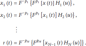
For more conventional signal distribution, the noise and the desired signal are in such a shape that we cannot find a single rotated coordinate system where we can completely eliminate the noise term from the signal. Thus, series of rotation of the coordinate system are needed and 3 may be generalized into a filter bank with consecutively changing orders:

$$\begin{array}{cc}& x_{\mathrm{1}}\left(t\right)=F^{-p_{\mathrm{1}}}\left\{F^{p_{\mathrm{1}}}\left[x\left(t\right)\right]H_{\mathrm{1}}\left(u\right)\right\},\\ x_{\mathrm{2}}\left(t\right)=F^{-p_{\mathrm{2}}}\left\{F^{p_{\mathrm{2}}}\left[x_{\mathrm{1}}\left(t\right)\right]H_{\mathrm{2}}\left(u\right)\right\},\\ ⋮\\ r\left(t\right)=F^{-p_N}\left\{F^{p_N}\left[x_{N-\mathrm{1}}\left(t\right)H_N\left(u\right)\right]\right\}.\end{array}$$

(6)

Furthermore, in the case where the $t\text{-}f$ distributions of noises and signals do not overlap in the $t\text{-}f$ plane, noises will be eliminated successfully by the filter designed by 6 as long as the transformation orders $p_1,p_2,\dots ,p_n$ are chosen properly. However, in the case of $t\text{-}f$ distributions overlapping, the filters may be selected in order to minimize the mean-square error.

3. The Determination of the Optimal Separating Lines on the Time-Frequency Plane

From the above analysis, it can be seen that the option of the separating line is nonuniqueness. Hence, how to find an optimal solution is the key to the filter design. In this paper, SVM classifiers, which often have superior recognition rates in comparison to other classification methods, are used to solve the parameters of the optimal separating lines in the $t\text{-}f$ plane. At first, the data model of the optimal classification problem is built by $t\text{-}f$ transformation. Then, in order to construct the training set, an image boundary extraction algorithm is adopted. After that, the parameters of the optimal separating line could be obtained by using SVM either in linear separability or in nonlinear separability.

3.1. Time-Frequency Image Representations

In order to locate signal and noise components in the $t\text{-}f$ plane accurately, the $t\text{-}f$ distribution of the observed signals should be achieved at first. The $t\text{-}f$ transformation in this paper should have a rotation relation with the FrFT, which is the essential foundation of the filter design in the u domain. It is known that the classical $t\text{-}f$ transformation such as the Gabor transform (GT), the WVD, and the ones derived from them such as the smoothing pseudo WVD (SPWVD) and the Gabor-Wigner transform (GWT) all satisfied the above property and their expressions are shown as follows:

$$\begin{array}{l}\text{GT:}\hspace{0.17em}\hspace{0.17em}{G}_s(t,f)={{\displaystyle \int }}_{-\infty }^{\infty }{e}^{-{\left(\tau -t\right)}^{\mathrm{2}}/\mathrm{2}}{e}^{-j\mathrm{2}\pi f\tau }s\left(\tau \right)d\tau ,\\ \text{WVD:}\hspace{0.17em}\hspace{0.17em}{W}_s(t,f)={{\displaystyle \int }}_{-\infty }^{+\infty }x(t+\frac{\tau }{\mathrm{2}})x^{*}(t-\frac{\tau }{\mathrm{2}})e^{-j\mathrm{2}\pi f\tau }d\tau ,\\ \text{SPWVD:}\hspace{0.17em}\hspace{0.17em}SP{W}_s(t,f)\\ \hspace{1em}={{\displaystyle \iint }}_{-\infty }^{+\infty }h\left(\tau \right)g\left(u\right)x\left(t-u+\frac{\tau }{\mathrm{2}}\right)x^{*}\\ \hspace{1em}\hspace{1em}\hspace{1em}\phantom{}\hspace{1em}·{\left(t-u+\frac{\tau }{\mathrm{2}}\right)}^{-j\mathrm{2}\pi f\tau }du\hspace{0.17em}d\tau ,\\ \text{GWT:}\hspace{0.17em}\hspace{0.17em}{C}_s\left(t,f\right)=G_s^{\mathrm{2.6}}\left(t,f\right)W_s^{\mathrm{0.6}}\left(t,f\right).\end{array}$$

(7)

The GT is considered as an example here to interpret the similarity between the $t\text{-}f$ plane and the 2D image. In the practical applications, the $t\text{-}f$ plane is represented in a Gabor coefficient matrix $X={\left(a_{mn}\right)}_{M\times N}$ which is obtained by the discrete GT for the samples of limited length signal and the element $a_{mn}$ ( $\left|a_{mn}\right|$ ) in the mth row and the nth column shows the distribution strengthen of observed signal at the point in the $t\text{-}f$ plane whose coordinates are ( $t_m,f_n$ ). Obviously, the $t\text{-}f$ plane is similar to a gray image so that each $t\text{-}f$ point corresponds to a pixel in the image and an $t\text{-}f$ image, which consists of three parts: signal areas, noise areas, and background, is obtained. Multidiscrete highlight energy concentration areas represent several signal and noises components that exist simultaneously and one of the most direct and effective way of separating these components is according to the edge of these highlight areas. As a result, the edges of these signals and noises, which could be detected by the boundary extraction technology, are suitable for the construction of the training set of SVM classifier.

3.2. Image Boundary Extraction in Time-Frequency Domain

As mentioned above, as a plain gray image, there are only several discrete highlight areas in the $t\text{-}f$ image and their edges are just some closed curves. Hence, by selecting the threshold reasonably, we can convert the gray image to its binary counterpart without losing useful information and the image boundaries could be obtained by edge extraction and thinning and smoothing algorithms, as shown in Figure 1(a). Then, all the edge pixels are coded in the binary image with integer numbers in sequence, from left to right, and then from top to bottom, so that pixel with small coordinate values could corresponds to a sole small integer number, as presented in Figure 1(b). After that, the given label number of each edge pixel with the numbers of the pixels in their eight neighborhoods is compared (the default label numbers of pixels which are not on the edge is zero) and the minimum value of these nine pixels is selected as the label number of the edge pixel, which is shown in Figure 1(c). However, though the label numbers of pixels that belong to the same edge are the same, there is no consequence among these labels of different edges. Hence, arrange these labels in sequential order and replace them by the sequence number in order to facilitate the edge selection. As can be seen, the edge labels are the numbers in the bracket of Figure 1(c).

Figure 1

The diagram of edge labeling (a) the binary image; (b) the label numbers of pixels; (c) the edge labels.

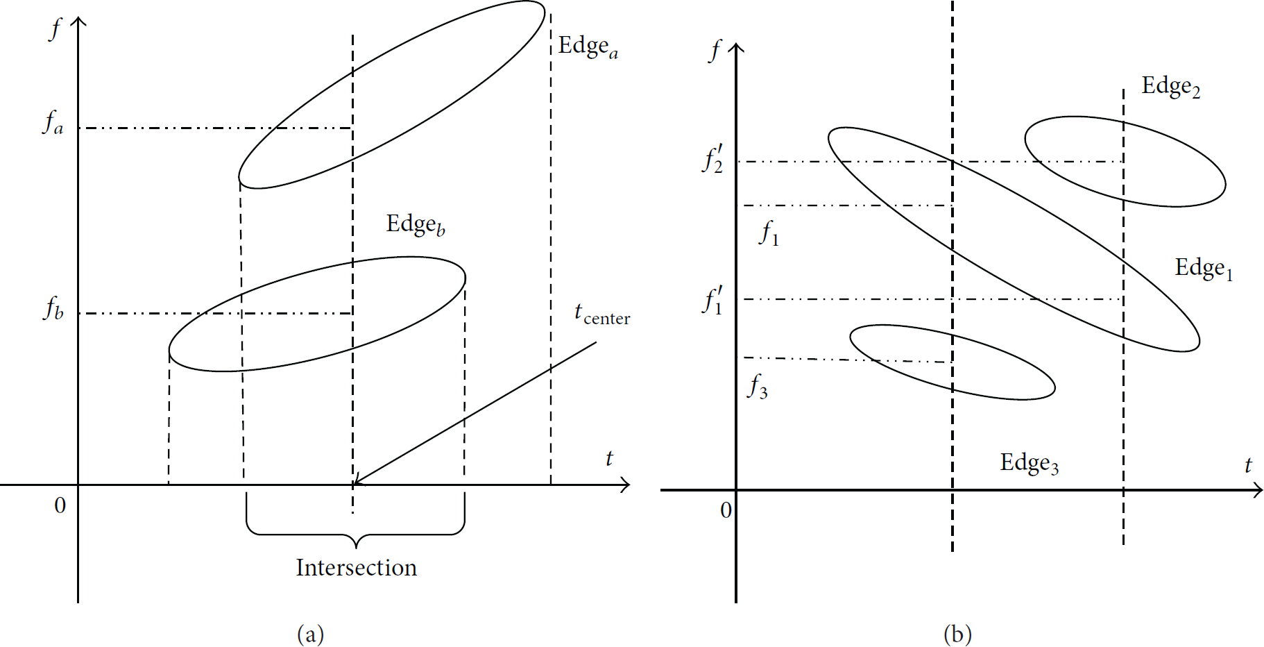
Considering the presence of false edges, sort all edges in descending order according to their length and select the first n edges where n is the total number of the noise and signal components because the false edges are always much shorter than actual edges. Then, the middle-value $t_{\text{center}}$ of the abscissa intersection of arbitrary two mutually coupled edges is calculated and the corresponding average f-values of these edges are obtained where the larger f-value corresponds to the larger label edge, as shown in Figure 2(a). The above operation is repeated until all edges are placed in order where an example is presented in Figure 2(b). Now, the adjacency of all n edges is obtained and there should exist separating lines between each two adjacent edges so that the edges on both sides of the separating line are constructed, the training set of the SVM classifier.

Figure 2

The diagram of adjacent edge selection. (a) the comparison between two coupled edges: because $f_a$ is larger than $f_b$ , the label of ${\text{Edge}}_a$ ( $L_a$ ) is larger than label of ${\text{Edge}}_b$ ( $L_b$ ); (b) ordering all edges: because $f_1>f_3$ , $f_2^{\prime }>f_1^{\prime }$ , so $L_1>L_3$ , $L_2>L_1$ , and the final order is $L_2>L_1>L_3$ and there are two separating lines, one is between $L_2$ and $L_1$ and the other one is between $L_3$ and $L_1$ .

3.3. The Parameters Determination of the Separating Line by SVM

The training set of SVM classifier is the following set of Q points:

$$\begin{array}{cc}& E=\{\left({\mathbf{x}}_q,c_q\right)\hspace{0.17em}|\hspace{0.17em}{\mathbf{x}}_q\in {\mathbf{R}}^{\mathrm{2}},\hspace{0.17em}\hspace{0.17em}{c}_q\in \left\{\mathrm{1},-\mathrm{1}\right\}\},\hspace{1em}q=\mathrm{1,2},\dots ,Q,\end{array}$$

(8)

where ${\mathbf{x}}_q$ is a 2D position vector representing the edge pixels in $t\text{-}f$ image obtained from the boundary extraction algorithm and $c_q$ indicates that the vector belongs to the different edges.

Hence, the training goal of the SVM classifier is to find an optimal separating line as in 9 so that the training set could satisfy the condition of correct classification as in 10 and the normalized margin $\mathrm{2}/‖\mathbf{w}‖$ is maximized. Consider

$$\begin{array}{cc}& f{\left(x\right)}_{\text{opt}}={\mathbf{w}}^T{\mathbf{x}}_q+w_{\mathrm{0}}^{\prime },\end{array}$$

(9)

$\begin{array}{cc}& c_q\left({\mathbf{w}}^T{\mathbf{x}}_q+w_{\mathrm{0}}^{\prime }\right)-\mathrm{1}\ge \mathrm{0},\hspace{1em}q=\mathrm{1,2},\dots ,Q.\end{array}$

(10)

The above problem is actually a convex quadratic programming which can be converted into its dual problem and be solved. N support vector $\{d_q\}$ and coefficients $\{a_q\}$ can be obtained from the SVM training and then we can use them to build the optimal support vector separating line equation.

In the case of linear separability, the optimal separating line is straight and defined by the following equation:

$$\begin{array}{cc}& f_l\left(x\right)={\displaystyle \sum }_{q=\mathrm{1}}^Q{c}_q{a}_q\left(x_q·x\right)+w_{\mathrm{0}}^{\prime },\end{array}$$

(11)

where $\left(x_q·x\right)$ is the dot product operation and the separating threshold $w_{\mathrm{0}}^{\prime }$ is the midvalue of any pair of support vector in different edges.

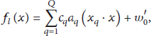
In the case of nonlinear separability, the inner production $K(x_q,x)$ of the support vector machine is needed instead of the dot product and Gaussian radial basis function is selected as the inner production in this paper so that the optimal separating line is a curve and the equation is

$$\begin{array}{cc}& f_c\left(x\right)={\displaystyle \sum }_{q=\mathrm{1}}^Q{c}_q{a}_{q}K\left(x_q,x\right)+w_{\mathrm{0}}^{\prime }.\end{array}$$

(12)

4. The Multiorder Fractional Filter Bank for Nonlinear Separability

It is obvious that, in the case of linear separability, the fractional filter as in 3 could be used directly so that, after getting the optimal separating line parameters by considering 4 and 11, the fractional filter can be constructed directly according to 5.

However, in the case of nonlinear separability, with the proper choice of SVM kernel function, an optimal separating curve is obtained which cannot assist FrFT filter design immediately. For this reason, a piecewise linear fitting algorithm may be used under a total least-square-error criterion where the curve is fitted to a set of linear segments connected end to end.

Provided that all M data points $(t,y_c(t))$ that belong to the separating curve $l_{\text{sep}\_c}$ have been known, the job is to solve the fitting function f:

$$\begin{array}{cc}& f=\frac{f_{n+\mathrm{1}}-f_n}{t_{n+\mathrm{1}}-t_n}\left(t-t_n\right)+f_n,\hspace{1em}{t}_n\le t\le t_{n+\mathrm{1}},\hspace{0.17em}\hspace{0.17em}n=\mathrm{1,2},\dots ,N,\end{array}$$

(13)

which satisfies

$$\begin{array}{cc}& {‖\delta ‖}^{\mathrm{2}}={\displaystyle \sum }_{m=\mathrm{1}}^M{\left[f_{\left(m\right)}\left(t\right)-y_{c\left(m\right)}\left(t\right)\right]}^{\mathrm{2}}=\min ,\end{array}$$

(14)

where $t_n$ and $f_n$ are the starting point and the inflection point of the nth segment and N is the segment number.

It is evident that f is more close to $f_c(x)$ and the separation effect of signal and noise is better with the increasing N. However, with the continuous increase of N, the order of filter bank and the degree of operation of FrFT also increase that would lead to high algorithm complexity. Furthermore, the discretization errors are accumulated in the repeated applications of DFrFT. As a consequence, the reasonable selection of N is an important impact on the performance of the filter and after that the parameters $t_n$ and $f_n$ could be determined by 14 and the filter of noise could be achieved by ( $N+1$ ) times FrFT and N times multiplicative filter by the serial filter bank in 6.

A more efficient parallel filter bank is proposed in this paper. At first, according to the fitting result, divide the observed signals in the time domain which may be divided into N parts where each part is corresponding to a segment of the fitted polyline; that is,

$$\begin{array}{l}x\left(t\right)={\displaystyle \sum }_{n=\mathrm{1}}^N{x}_n\left(t\right),\\ x_n\left(t\right)=x\left(t\right),\hspace{1em}{t}_n\le t<t_{n+\mathrm{1}},\hspace{1em}{x}_n\left(t\right)=\mathrm{0},\hspace{1em}\text{others}.\end{array}$$

(15)

Then, after determination of the transformation order and transfer function of each sub-filter, each fitting segment $x_n(t)$ may be filtered separately and the output is superimposed as the ultimate recovered signal $r(t)$ ; that is,

$$\begin{array}{cc}& r\left(t\right)={\displaystyle \sum }_{n=\mathrm{1}}^N{F}^{-p_n}\left\{F^{-p_n}\left[x_n\left(t\right)\right]H_n\left(u\right)\right\}.\end{array}$$

(16)

5. Application: Cross-Term Elimination in Wigner Distribution

The Wigner distribution function is succinct which satisfies many good mathematics properties and one of which is the excellence of $t\text{-}f$ focusing property, whereas, there is a problem for the WD; that is, “the cross-term problem.” This problem makes it difficult to distinguish between signal parts, noise parts, and the cross-term part of the WD so that WD is improper for the cases where the signal consists of several $t\text{-}f$ components.

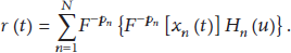
Pei and Ding presented a method to detect and eliminate the WD cross-term based on the $t\text{-}f$ rotation characteristic of FrFT which could obtain the optimal autoterm resolution even that there are overlapping areas between the autoterms and the cross-terms [15]. However, it is an iteration-search algorithm which has a complexity computation and the inherent serial structure is hard to hardware implementation. Here, an algorithm based on this factional filter is proposed and the flowchart is shown as Figure 3. This method could completely eliminate the cross-term in WD and the time-frequency distribution that we get in the end high resolution and good readability which could also work well when autoterms and cross-terms overlap. Furthermore, the lower computation and more efficient parallel structure may be more easily implemented at engineering. The detailed procedure is as follows.

• (1)

The observed signal is transformed by GT and a blur $t\text{-}f$ image without cross-terms is shown in the $t\text{-}f$ plane containing multidiscrete highlight energy concentration areas which represent signal or noise components.

(2)

The obtained GT gray image is converted to its binary counterpart by the efficient threshold selection method and then the image boundary extraction technology is used to select the edges of signal and noise areas which construct the training set of SVM classifier.

(3)

The different areas in the $t\text{-}f$ image are classified and the parameters of optimal separating lines are determined by SVM. If there are more than two components in the observed signal, that is, $M>2$ , the one-versus-rest SVMs should be constructed and the areas of different components are separated gradually.

(4)

According to the optimal transformation order and the transfer function of the filter (bank) which are determined by the parameters of the optimal classified line function (or functions), each signal (or noise) component in $t\text{-}f$ plane and then in t domain could be obtained.

(5)

Each filtered component is individually transformed in the $t\text{-}f$ plane again.

(6)

All these $t\text{-}f$ distribution outputs are added together in the $t\text{-}f$ plane, and a high-clarity $t\text{-}f$ image without cross-terms is obtained.

Figure 3

The flowchart of the WD cross-term elimination algorithm.

Furthermore, the proposed fractional filter could be used in many other applications besides cross-term elimination in Wigner distribution. For example, it can be also applied in the research on the moving targets detection and imaging by airborne synthetic aperture radar which needs further research.

6. Simulation

6.1. The Selection of Time-Frequency Distribution

An observed signal $x(t)$ as in 17 is considered as follows:

$$\begin{array}{l}x\left(t\right)=s\left(t\right)+n\left(t\right)=e^{-t^{\mathrm{2}}/\mathrm{4}}{e}^{j\pi \left(\mathrm{8}{t}^{\mathrm{2}}+\mathrm{70}t\right)}+e^{-t^{\mathrm{2}}/\mathrm{4}}{e}^{j\pi \left(\mathrm{8}{t}^{\mathrm{2}}+\mathrm{40}t\right)},\end{array}$$

(17)

where $s(t)$ is a Gaussian amplitude modulated linear frequency modulated (LFM) signal with the additive noise $n(t)$ . The observation time is from −2 s to 2 s and the sampling rate $f_s$ is 100 Hz. WVD, GT, SPWVD, and GWT of $x(t)$ are shown separately in Figures 4(a)–4(d). It is obvious that the signal and noise present coupling either in the time domain or the frequency domain, though they have different $t\text{-}f$ focusing properties under different $t\text{-}f$ transforms.

Figure 4

The time-frequency distribution of the observed signal. (a) WD; (b) GT; (c) SPWVD; (d) GWT.

The comparison of fractional filter performance under different $t\text{-}f$ transforms is shown in Table 1, where IF is the SNR improvement factor and MSE is the mean square error of recovered signal; that is,

$$\begin{array}{cc}& \text{IF}=\frac{\text{SN}{\text{R}}_{\text{out}}}{\text{SN}{\text{R}}_{\text{IN}}},\\ \text{MSE}=\frac{\int {\left|r\left(t\right)-s\left(t\right)\right|}^{\mathrm{2}}dt}{\int {\left|s\left(t\right)\right|}^{\mathrm{2}}dt}.\end{array}$$

(18)

Table 1

$t\text{-}f$ filter performances versus different $t\text{-}f$ transforms.

	MSE (%)	IF (dB)	Training sample number of SVM
WVD	0.1083	29.6528	334
GT	0.1087	29.6382	394
SPWVD	0.1084	29.6496	396
GWT	0.1083	29.6531	327

Under these four classic $t\text{-}f$ transforms, it can be seen that, though the $t\text{-}f$ images and the boundaries of components are different, all the filters are able to recovery the signal successfully so that the fractional filter design method proposed in this paper is not limited to any particular $t\text{-}f$ transformation. When WVD or GWT is adopted, the fewer training sample number of SVM and a little better filtering effect are obtained. However, the cross-term in WVD could be avoided by using the method proposed in Section 5 but may increase the calculation. Hence, GWT will be adopted in the following experiments.

6.2. In the Case of Linear Separability

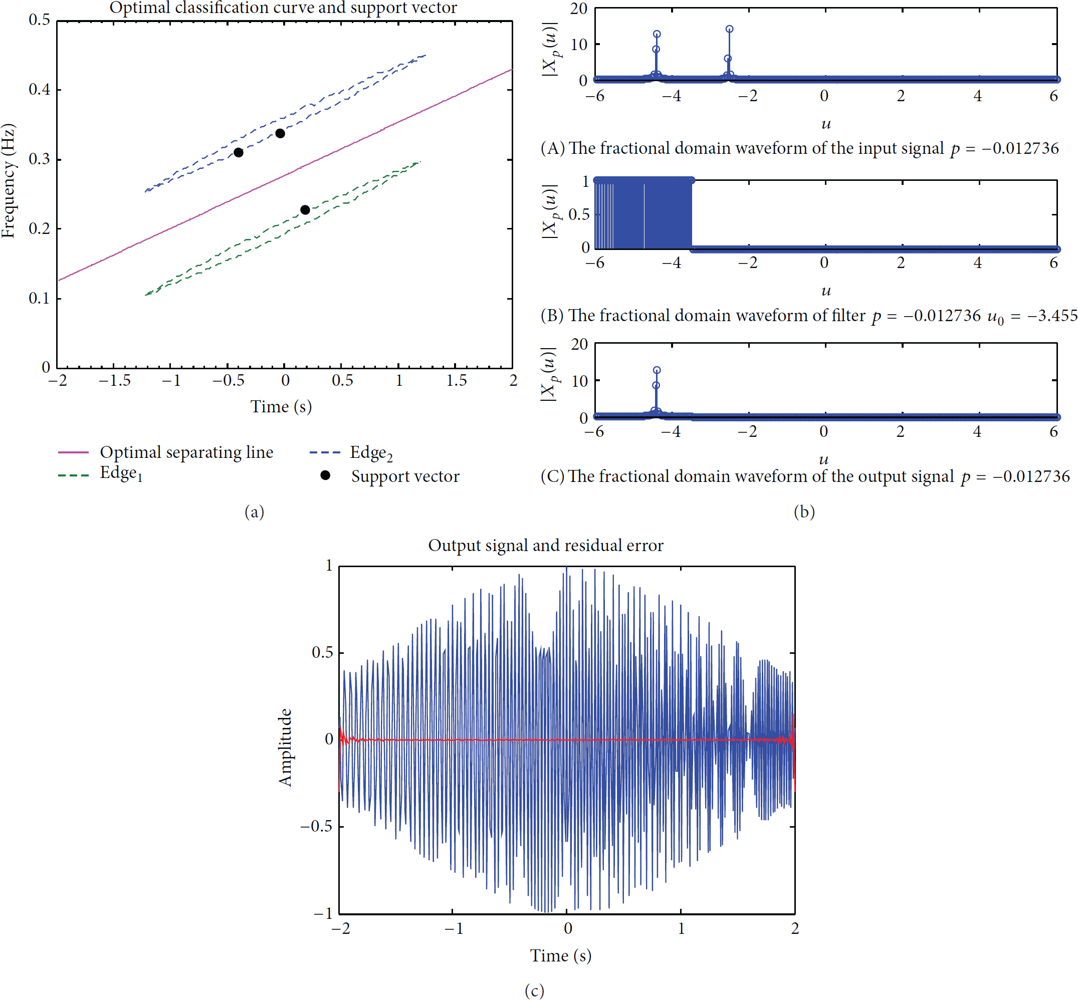
The input signal $x(t)$ and the GWT of $x(t)$ are shown in 17 and Figure 4(d). Through the boundary extraction algorithm, the edges of signal and noise can be selected as the SVM training set which are dashed lines in Figure 5(a). Based on these edges, the support vector and optimal separating line are obtained, which are shown in Figure 5(a) with black dots and solid line, and the separating line equation is l: $f(x)=0.0795x+0.2765$ . Figure 5(b) shows the process of filter in the u domain where parameters of the fractional filter are $p=0.012736$ and $u_0=-3.455$ , and the recovered signal and residual error are shown in Figure 5(c). As can be seen from the above results, the noise can be filtered effectively by using our design method in the case of linear separability.

Figure 5

The filtering process: (a) optimal separating line and support vector; (b) filtering in fractional domain; (c) recovered signal and recovered error.

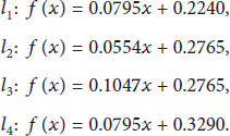
In order to evaluate the influence of the filter performance from the optimal characteristic of separating line, four typical nonoptimal separating lines are constructed as shown in Figure 6 and the equations are

$$\begin{array}{l}{l}_{\mathrm{1}}\text{:}\hspace{0.17em}\hspace{0.17em}f\left(x\right)=\mathrm{0.0795}x+\mathrm{0.2240},\\ l_{\mathrm{2}}\text{:}\hspace{0.17em}\hspace{0.17em}f\left(x\right)=\mathrm{0.0554}x+\mathrm{0.2765},\\ l_{\mathrm{3}}\text{:}\hspace{0.17em}\hspace{0.17em}f\left(x\right)=\mathrm{0.1047}x+\mathrm{0.2765},\\ l_{\mathrm{4}}\text{:}\hspace{0.17em}\hspace{0.17em}f\left(x\right)=\mathrm{0.0795}x+\mathrm{0.3290}.\end{array}$$

(19)

Figure 6

Four typical nonoptimal separating lines.

According to these four separating lines, fractional filters are constructed and the filter performances are shown in Table 2. It can be seen that the performance of the filter designed by SVM is better than that based on other separating lines because the truncation of the observed signal in the time domain and the picket fence effect of discrete spectral analysis cause the energy leakage of signals and noises to the entire $t\text{-}f$ plane, while the SVM classifier maximizes the margin in order to separate the signals and noises in the $t\text{-}f$ domain to the most degree.

Table 2

$t\text{-}f$ filter performances versus different separating lines.

Operating line	l	$$l_1$$	$$l_2$$	$$l_3$$	$$l_4$$
MSE (%)	0.1083	0.1403	0.1715	0.1724	0.2158
IF (dB)	29.6531	28.5298	27.6558	27.6362	26.6720

6.3. In the Case of Nonlinear Separability

In this case, the observed signal $x(t)$ consisted of a quadratic frequency modulated signal $s(t)$ with noise $n(t)$ :

$$\begin{array}{l}x\left(t\right)=s\left(t\right)+n\left(t\right)=e^{-t^{\mathrm{2}}/\mathrm{100}}{e}^{j·\mathrm{2}\pi \left(\mathrm{0.023}{t}^{\mathrm{3}}+\mathrm{4.5}t\right)}\\ +e^{-t^{\mathrm{2}}/\mathrm{100}}{e}^{j·\mathrm{2}\pi \left(\mathrm{0.01}{t}^{\mathrm{3}}+\mathrm{2}t\right)}.\end{array}$$

(20)

The observation time is from −10 s to 10 s and the sampling rate $f_s$ is 30 Hz. Figure 7(a) shows the GWT of $x(t)$ where the two components in the $t\text{-}f$ plane could not be separated by a straight line and the optimal separating curve is shown in Figure 7(b). As mentioned in Section 4, the curve should be fitted to a set of linear segments and the segment number N is a key to design the fractional filter bank. The value of coefficient of determination $R^2$ is adopted to measure the goodness of fit which is defined as follows:

$$\begin{array}{cc}& R^{\mathrm{2}}=\mathrm{1}-\frac{S{S}_{\mathrm{err}}}{S{S}_{\text{tot}}}=\mathrm{1}-\frac{{\sum }_{m=\mathrm{1}}^M{\left[y_{c\left(m\right)}-f_{\left(m\right)}\right]}^{\mathrm{2}}}{{\sum }_{m=\mathrm{1}}^M{\left[y_{c\left(m\right)}-{\bar{y}}_{c\left(m\right)}\right]}^{\mathrm{2}}},\end{array}$$

(21)

where $S{S}_{\mathrm{err}}$ is the residual sum of squares (RSS), $S{S}_{\mathrm{err}}$ is the total sum of squares (TSS), and $y_{c(m)}$ , $f_{(m)}$ , and ${\bar{y}}_{c(m)}$ are the data of the optimal separating curve, the fitting data, and the average of $y_{c(m)}$ , respectively.

Figure 7

Filtering experiments in the case of nonlinear separability. (a) GWT of $x(t)$ ; (b) the optimal classification curve and support vector; (c) 4th-order fitting of SVM separating line; (d) recovered signal and recovered error.

Table 3 shows the value of $R^2$ versus different segment number N. It can be seen that when $N=4$ , the fitting linear segments have a very high fitting precision, while $N=3$ already satisfies most practical cases. The 4th-order fitting of SVM separating line is shown in Figure 7(c) and the fitting equation is

$$\begin{array}{cc}& f\left(x\right)=\left\{\begin{array}{cc}-\mathrm{0.0218}x+\mathrm{0.0277},\hfill & -\mathrm{10}\le x<-\mathrm{5.2069},\hfill \\ -\mathrm{0.0071}x+\mathrm{0.1041},\hfill & -\mathrm{5.2069}\le x<\mathrm{0.0577},\hfill \\ \mathrm{0.0073}x+\mathrm{0.1032},\hfill & \mathrm{0.0577}\le x<\mathrm{5.4024},\hfill \\ \mathrm{0.0223}x-\mathrm{0.0222},\hfill & \mathrm{5.4024}\le x\le \mathrm{10}.\hfill \end{array}\right.\end{array}$$

(22)

Table 3

The value of $R^2$ versus different segment number N.

N	1	2	3	4	5	6	7
$$R^2$$	0.0001	0.9301	0.9872	0.9958	0.9975	0.9981	0.9987

Calculate IF and $\text{MSE}$ with $N=4$ , and the result is $\text{IF}=25$ .5421 dB, $\text{MSE}=0.1828\%$ . The recovered signal and residual error are shown in Figure 7(d). As can be observed in the above results, the proposed algorithm still achieves an effective noise filtering in the case of nonlinear separability, while the performance degradation caused by the errors of piecewise linear fitting and the discrete multiorder filter bank cannot be helped.

6.4. Cross-Term Elimination in Wigner Distribution

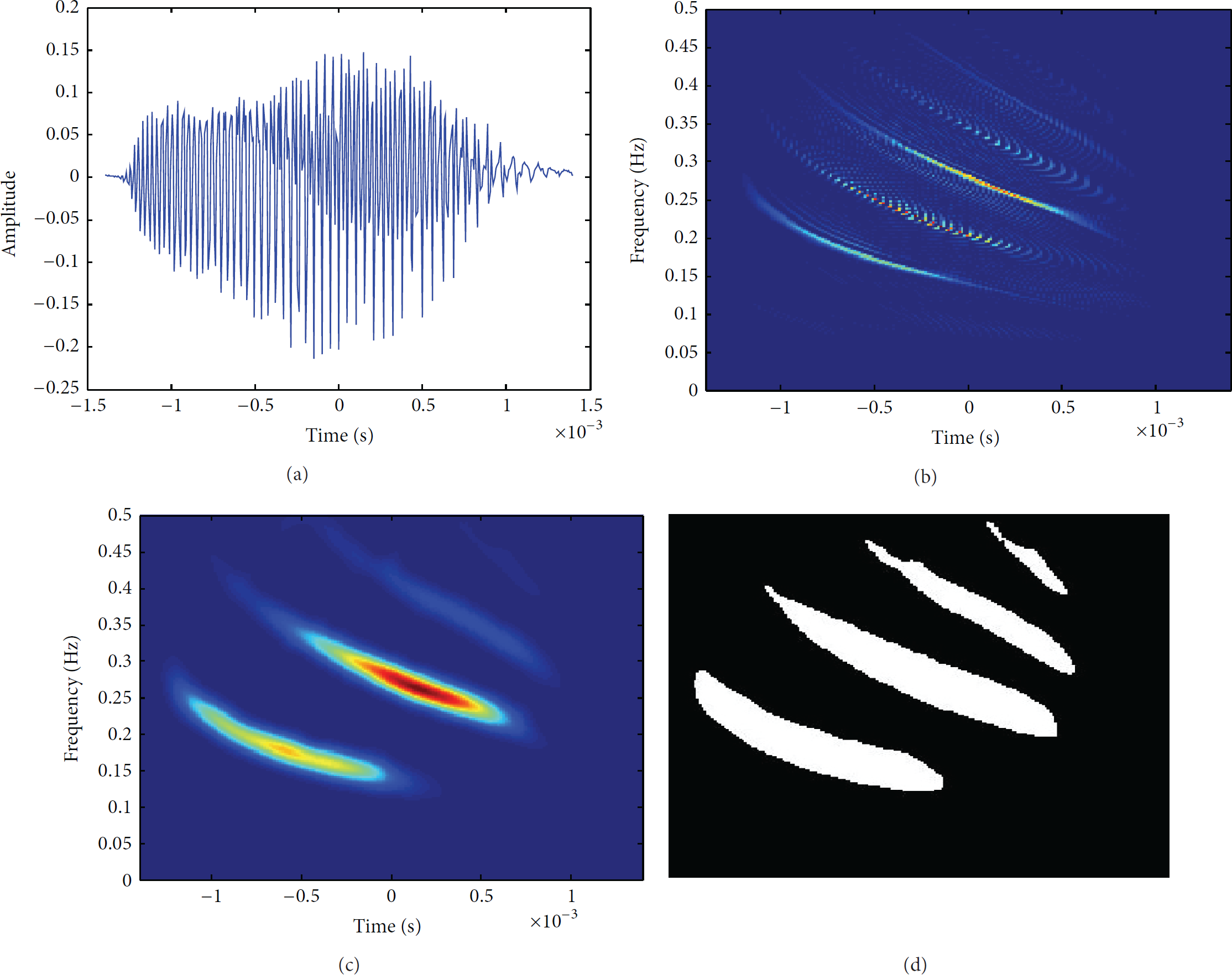
The observed signal $x(t)$ is the digitized echolocation pulse emitted by the large brown bat, Eptesicus fuscus. There are 400 samples and the sampling period is 7 ms [14]. The time domain waveform is given in Figure 8(a).

Figure 8

(a) The time domain waveform of $x(t)$ ; (b) the WVD of $x(t)$ ; (c) Gabor of $x(t)$ ; (d) the binary image of $x(t)$ .

As can be seen from Figure 8(b), there are many cross-terms in the WVD of $x(t)$ and the difference between the intensity of each component is large where the weak components are submerged by the strong components and cross-terms so that the readability of the $t\text{-}f$ image is poor. The Gabor of $x(t)$ has no cross-term though the image is blurring, which is shown in Figure 8(c). The threshold is determined by the characteristics of the $t\text{-}f$ image and the binary image is shown in Figure 8(d). It is obvious that there are four different components in the binary image so that they could be separated individually by our fractional filter bank. The optimal separating lines and the filtering process are shown in Figure 9.

Figure 9

The support vector and the optimal separating line. (a) $f(x)=-92.214x+0.2094$ ; (b) $f(x)=-146.07x+0.4701$ ; (c) $f(x)=-128.89x+0.3558$ .

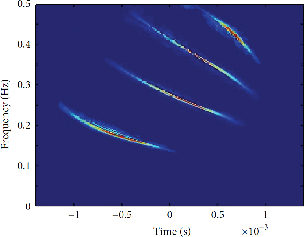
The GWT of all single components, which is obtained from filtering one by one, is calculated and superimposed so that a clear image without cross-term is achieved as shown in Figure 10. It can be seen that our design method can avoid the cross-term completely and not affect the quality of the autoterms. Meanwhile, it is effective even in the case of overlap between the autoterms and the cross-terms. Furthermore, the $t\text{-}f$ image is more readable because the weak components are strengthened in the conversion process from the gray image to the binary image.

Figure 10

The clear $t\text{-}f$ image of $x(t)$ without cross-term.

7. Conclusion

A novel general design of fractional filter is proposed in order to realize the lossless recovery of nonstationary signal in complicated noise environment. The estimation procedures for the parameters of the optimal separating lines in the case of linear separability and those of the optimal separating curves in the case of nonlinear separability in the $t\text{-}f$ plane are given in detail and the specific design methods in both of these two cases are presented. This design is versatility and can ensure the optimal performance of the filter without any statistic priori knowledge. Simulation results show that it still works well even in the case of strong coupling between the signal and noise and do not depend on the selected $t\text{-}f$ transformation. Furthermore, our fractional filter can realize the effective elimination of the cross-term in WD and $t\text{-}f$ image rich in detail can be achieved.