
Abstract
Aiming at solving the problem of low accuracy in traditional distance vector-hop (DV-hop) algorithm used for wireless sensor networks node location, two refined localization algorithms, that is, hyperbolic-DV-hop localization algorithm and improved weighted centroid DV-hop localization algorithm (IWC-DV-hop), are proposed in this paper. Instead of taking the average HopSize of BeaconNode nearest to the UnknownNode, hyperbolic-DV-hop algorithm chooses the average of average HopSizes of all BeaconNodes, as the average HopSize of the UnknownNode. The ML localization algorithm is also replaced by hyperbolic location algorithm. IWC-DV-hop algorithm improves the accuracy by selecting appropriate BeaconNodes and replacing ML localization with centroid localization. And a weighted scheme is used in IWC-DV-hop so that the influence of different anchors is taken into consideration. Simulations have been conducted to prove that the accuracy is improved by both of the two algorithms and IWC-DV-hop is the best choice.
1. Introduction
Wireless sensor network (WSN) is an increasingly important technology attracting considerable research interest. WSNs consist of thousands of nodes with built-in sensors which can collect a variety of information from surrounding environment. Localization is one of the most important problems in WSNs, for position information is needed in all kinds of situations [1]. In environmental monitoring applications such as bush fire surveillance, water quality monitoring, and precision agriculture, the measurement data are meaningless without knowing the location from where the data are obtained. Moreover, location estimation may enable a myriad of applications such as inventory management, intrusion detection, road traffic monitoring, health monitoring, reconnaissance, and surveillance. Sensor network localization algorithms estimate the locations of sensors with initially unknown location information by using knowledge of the absolute positions of a few sensors and intersensor measurements such as distance and bearing measurements [2]. GPS is widely used for localization, but it is impossible for WSNs to be used considering the cost limitation. So we need some special localization algorithm for WSNs.
Currently, there are many kinds of self-localization algorithms [3], which can be divided into two categories, that is, range-based and range-free [4].
Range-based algorithms use absolute point-to-point distance or angle information to calculate distance between neighbouring sensors [5]. Although the use of range measurements results in a fine-grained localization scheme, range-based algorithms require the sensor to contain additional hardware to make range measurements. There are many common range-based localization algorithms such as received signal strength indicator (RSSI) [6], time of arrival (TOA) [7], time difference of arrival (TDOA) [8], and angle of arrival (AOA) [9].
Range-free algorithms do not need absolute range information. The accuracy is much lower than the range-based but it can still satisfy many applications’ requirements. Hardware requirement of range-free algorithms is little; it does not need actual measurements of physical properties like radio signal strengths, angle of arrival of signal, and distance, so the range-free algorithms are more economical, cost-effective, and feasible for the large-scale wireless sensor networks. There are many range-free localization algorithms, such as centroid algorithm [10], DV-hop [11, 12], amorphous [13], APIT [14], and MDS-MAP [15, 16].
WSN devices have a hardware limitation that is why solutions of range-free localization are being pursued as a cost-effective method compared to other more expensive range-based approaches [17]. In this paper we focus on DV-hop, one of the range-free localization algorithms.
Extensive research has been done on the application of DV-hop algorithm since the algorithm was first proposed by Niculescu and Nath in 2001 [6, 7]. It is still very popular due to its simplicity, cost-effectiveness, and robustness. Therefore researchers keep working on its improvement.
In [18], Dulman and Havinga discussed the influence of the underlying random topology, and based on that they derived a distance estimation function of the hop count by which two nodes are separated and characterized the precision of these estimations. And they obtained the improvement of roughly 26% for DV-hop localization algorithm in position accuracy.
Checkout DV-hop algorithm and selective 3-anchor DV-hop algorithm were proposed by Gui et al. A calculation step, called checkout step, was added to DV-hop in checkout DV-hop [19]. In selective 3-anchor DV-hop algorithm, the normal node first selects any three anchors to form a 3-anchor group; then it calculates the candidate position based on each 3-anchor group, and finally according to the relation between candidate positions and the minimum hop counts to anchors, the normal node chooses the best candidate position [20].
DV-hop + Lastdist algorithm was proposed by Zhang et al. in [21]. A distance variable of final hop was added to the DV-hop communication message. The distance from the node to the anchor node can properly reduce the error distance caused by the final hop.
WD-DV-hop was proposed by Lin et al. in [22]. The centralized and distributed calculation method is replaced by a weighted calculation method. The distance between unknown nodes and anchor nodes is calculated by a method, in which the average one-hop distance of each anchor node multiplies by hops count between unknown nodes and anchor node.
There are also some researchers working on centroid localization algorithm. In [23] Deng et al. applied his improved centroid localization algorithm in WSN. He proposed a centroid algorithm with selected anchor node localization algorithm (SA-Centroid) for WSNs. The triangle centroid and polygon centroid were used and the method of selecting nearest anchor node was adopted. However, the SA-Centroid is complex and the amount of calculation is huge. Furthermore the accuracy improvement is limited. Based on the related work above, we proposed our DV-hop algorithm, which is simpler and provides better localization accuracy.
The rest of this paper is organized as follows. In Section 2, we briefly review two other researchers’ study on DV-hop's improvement which we have realized. In Section 3, original DV-hop localization algorithm is briefly introduced. In Section 4, we introduce how we refine DV-hop, and the simulation results are illustrated in Section 5. We also compare and analyze the difference between original DV-hop and our two algorithms, as well as the difference between our two algorithms and other improved DV-hop algorithms. Finally, we present our conclusions in Section 6.
2. Related Works
In [24], Li et al. proposed an improved DV-hop algorithm, named weighted DV-hop algorithm (WDV-hop). Jian Li's algorithm is derived from DV-hop algorithm and uses weight of anchors to improve localization accuracy without any additional hardware device. Jian Li's algorithm gives every anchor a weight which reflects the effects of anchor. In Jian Li's algorithm an unknown node computes the hop-size based on all the hop-size values it receives from the anchors, instead of just taking the first received hop-size value as in original DV-hop algorithm. Using this strategy, the position of unknown nodes is calculated by using weighted least square method.
In [25], Zhang et al. analyse the drawback of DV-hop and centroid location algorithm and proposed a new weighted centroid algorithm based on DV-hop, named weighted centroid localization algorithm (WCL). Their algorithm uses weight of anchors to improve accuracy. Every anchor node is weighted by a value reflecting the effect of the anchor node on the unknown node.
We have realized these two algorithms by programming with MATLAB so that we can compare our proposed algorithms with them from lots of aspects. The comparison and analysis will be made after we introduce our algorithms in following sections.
3. Theoretical Background
In this paper, we focus on static networks, where nodes do not move, since this is already a challenging condition for distributed localization. We assume that some anchor nodes, named BeaconNode, have a priori knowledge of their own positions. Note that anchor nodes have the same capabilities (processing, communication, energy consumption, etc.) as all other sensor nodes with unknown positions, which are named UnknownNode.
3.1. DV-Hop Localization Algorithm
The traditional DV-hop algorithm was developed by Niculescu and Nath [6, 7]. It can be summarized as in the following three steps.
3.1.1. Finding the Minimum HopCount
In the first step, all BeaconNodes broadcast beacon messages to other nodes; the format of the beacon message is
3.1.2. Calculation of the Distance between BeaconNodes and UnknownNodes
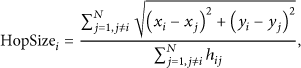
In the second step, the BeaconNodes get minimum HopCount value to other BeaconNodes according to the result in the first step. Then it can estimate average HopSize to other BeaconNodes on the basis of the minimum HopCount and the distance between BeaconNodes. The
3.1.3. Calculation of Estimated Location
In the third step, the UnknownNode can calculate their locations by maximum likelihood (ML) estimation [26] or trilateration. In this paper we choose ML estimation and it will be introduced in the next section.
3.2. Maximum Likelihood Estimation
ML estimation is a good way to calculate UnknownNodes’ locations [4, 5, 27, 28]. With its help, we can obtain the following set of the equations:


3.3. Centroid Localization Algorithm
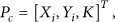
This section is devoted to the centroid algorithm. It is the most basic schemes, and it comprises three stages. First, BeaconNodes broadcast the localization reference to its neighbourhoods. In the second stage, the UnknownNodes receive and restore the information transmitted by at least three different BeaconNodes and then, classical arithmetic mean is employed to calculate the position of UnknownNode. Each UnknownNode maintains a table {beacon's id, position of the beacon
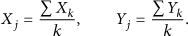
Figure 1 shows the detailed interpretation of the centroid algorithm. In centroid algorithm based positioning, the UnknownNode's estimation coordinate is the centroid of the polygon formed by BeaconNodes. Suppose that there are five BeaconNodes around the UnknownNodes


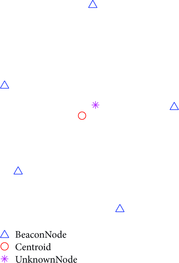
The concept of centroid algorithm.
4. Improvement of DV-Hop Localization Algorithm
In this section, we present two enhanced DV-hop algorithms, that is, hyperbolic-DV-hop localization algorithm and IWC-DV-hop localization algorithm. The original DV-hop takes the average HopSize of BeaconNode nearest to the UnknownNode, which is believed to be the reason leading to large errors. So we replace it with the average of average HopSizes of all BeaconNodes, as the average HopSize of the UnknownNode. The ML localization algorithm is replaced by Hyperbolic location algorithm, which has better performance results. In IWC-DV-hop algorithm, centroid algorithm is combined with DV-hop algorithm, and a weighted scheme is used in IWC-DV-hop so that the influence of different anchors is taken into consideration.
4.1. Our Hyperbolic-DV-Hop Localization Algorithm
After a thorough study of the principle of original DV-hop localization algorithm, we found that the errors of original DV-hop localization algorithm are caused by HopCounts, averaging HopSizes, and localization algorithm. So we managed to improve it through working on the last two steps, that is, the way to calculate distance between BeaconNode and UnknownNode and the localization algorithm.
4.1.1. Refinement on Second Step—Distance Estimation
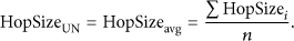
As what we have introduced above, UnknownNodes, in original DV-hop algorithm, take the average HopSize of its nearest BeaconNode as their own average HopSize. But the nodes in the WSN are disposed stochastically, which means the path between nodes may be not straight, which is the reason why the average HopSizes are always bigger than the actual value.
When the distance between UnknownNode and BeaconNode is calculated using the average HopSize, the error is always large. The nearest BeaconNode is unique and cannot be used to represent the whole BeaconNodes. Since ML in the third step will make use of the distance between UnknownNodes and every BeaconNode, it is a good way to take the average HopSize of all BeaconNodes to replace that of the nearest BeaconNode for UnknownNodes.
We calculate the average HopSizes of all BeaconNodes by

4.1.2. Refinement on Third Step—Location Algorithm
In the original DV-hop algorithm, ML or trilateration is used for physical distances estimations. In this paper, we use hyperbolic location algorithm [29, 30] to replace ML.
We derive the following expression:

Set


4.2. Our Improved Weighted Centroid DV-Hop Localization Algorithm
The accuracy improvement of Hyperbolic-DV-hop localization algorithm is still limited, so we have further proposed our improved weighted centroid DV-hop localization algorithm. Firstly, we simply replace the hyperbolic algorithm with centroid algorithm. Secondly, we analyse the reason leading to errors and then offer our solutions which turn out to improve the accuracy.
4.2.1. Refinement on the Third Step—Using Centroid Algorithm to Calculate the UnknownNodes’ Location
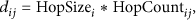
In the second step in original DV-hop algorithm, we can get the distance,
4.2.2. Further Analyses of the Reason for Error in DV-Hop
We have discussed one of the reasons why the error exists in original DV-hop in Section 4.1; that is, the original DV-hop takes the average HopSize of BeaconNode nearest to the UnknownNode. We replace it with the average of average HopSizes of all BeaconNodes, as the average HopSize of the UnknownNode. But the improvement of accuracy is limited. After further analysing the DV-hop algorithm, we found that error can be further reduced by adopting a new method.
In the second step of the original DV-hop, UnknownNode uses 2 to calculate the distance between itself and BeaconNodes. The distance can also be calculated by multiplying BeaconNodes’ HopSize by HopCount from another perspective. In other words, the HopSize of UnknownNodes is not necessary anymore. That means we can cut out one little step from the second step of DV-hop.
4.2.3. Refinement on the Second Step of DV-Hop
The HopSize of UnknownNode is not needed anymore and the step to calculate the HopSize of UnknownNode is cut out. The

The accuracy will be improved since the total number of steps for localization is decreased. From mathematical point of view, the calculation result will be less accurate in the case where an estimated value is calculated (added, subtracted, multiplied, divided, etc.) for
4.2.4. Further Analyses of the Reason for Error in Centroid Algorithm
In the centroid algorithm, the unknown node's estimation coordinate is the centroid of the polygon formed by BeaconNodes. And centroid algorithm cannot reflect the influence of the distance between BeaconNodes and UnknownNodes. In fact, the BeaconNodes which are closer to the UnknownNode will have a greater impact on the UnknownNode. Different BeaconNodes have different effect on the UnknownNode, considering the distance between them. But the centroid algorithm treats them as the same kind of node. In order to embody the effect of BeaconNodes which have different distance on the accuracy calculation, our improved weighted centroid DV-hop (IWC-DV-hop) algorithm is proposed.
4.2.5. Refinement on the Centroid Algorithm
As what 2 and 21 have showed, distance between BeaconNodes and UnknownNodes has a direct correlation with HopCounts. So the effect of distance on accuracy can be replaced by HopCounts. Then we can calculate the location of UnknownNodes by
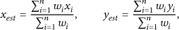
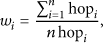
Another advantage with our improvement to the original centroid algorithm is that without threshold the weighted solution can make full use of all BeaconNodes available. While only those BeaconNodes whose
5. Simulation and Performance Comparison
We compare the performance of different locating methods by evaluating the average location error for each algorithm. The performance comparisons are conducted using a simulator developed with MATLAB R2013a, and all the nodes are deployed in a 500 m * 500 m area.
The comparison with other two researchers’ algorithms has also been made in this section. We have realized their algorithms by programming according to their description in [24, 25].
5.1. Varying the BeaconNode Ratio
Firstly we compare the performance of three localization algorithms with different BeaconNode ratios. Suppose the number of all nodes is 800, and the communication radius of BeaconNode is 100 m. We calculated the average of results of 50 simulations and set the average as the error ratio. Gradually, we increased the ratio of BeaconNode and get the different results in different situations.
The performance comparison with 3 different localization algorithms is shown in Figure 2. The upper line shows the error ratio of original DV-hop algorithm varies with the increase of the BeaconNode ratio, while the middle line shows the error ratio of hyperbolic-DV-hop algorithm and the lower line shows the error ratio of our IWC-DV-hop. It is obvious to observe that our IWC-DV-hop algorithm is much superior to the other two. In fact, the accuracy improvement of our hyperbolic-DV-hop over the original DV-hop is 8.2%, while our IWC-DV-hop over the original DV-hop is 63%.

Comparison with different BeaconNode ratios.
Figure 3 shows the comparison between our hyperbolic-DV-hop algorithm, our IWC-DV-hop algorithm, Jian Li's WDV-hop algorithm in [24], and Bingjiao Zhang's WCL algorithm in [25]. Overall, it is obvious that our IWC-DV-hop algorithm performs best with the least error ratio. We can also conclude that our proposed two algorithms are more stable, for their fluctuation range is smaller with the variety of BeaconNode ratio than that of Jian Li's WDV-hop algorithm and Binjjiao Zhang's WCL algorithm. In addition, the environment with low density of BeaconNodes is simulated and compared. The result shows that our IWC-DV-hop algorithm still has the best accuracy and is qualified for this kind of environment.

Comparison with different BeaconNode ratios.
5.2. Varying Node Number
When we compare the performance of three localization algorithms with different nodes number, we set the BeaconNode ratio to 50% and communication radius to 100 m. We calculated the average of results from 50 simulation experiments and set the average as the error ratio. Furthermore, we increased nodes number from 300 to 800 to get the different results in different situations.
Figure 4 illustrates the contrast with three different algorithms with different nodes number. The upper line shows the error ratio of original DV-hop algorithm varies with the increase of the nodes number, while the middle line shows the error ratio of hyperbolic-DV-hop algorithm and the lower line shows the error ratio of our IWC-DV-hop. We observe that, to a certain extent, the hyperbolic algorithm improves the accuracy, while the IWC-DV-hop algorithm improves the accuracy on a much larger scale. The accuracy improvement of our hyperbolic-DV-hop over the original DV-hop is 10.3%, while our IWC-DV-hop over the original DV-hop is 59%.

Comparison with different node number.
Figure 5 shows the relationship between error ratio and node number. In this simulation, we compare the accuracy of our proposed hyperbolic-DV-hop, our proposed IWC-DV-hop algorithm, Jian Li's WDV-hop algorithm in [24], and Bingjiao Zhang's WCL algorithm in [25]. This simulation result has proven the validity of IWC-DV-hop, since it always has the least error ratio and fluctuation.

Comparison with different node number.
5.3. Varying Communication Radius
In this scenario, we investigate the impact of increasing communication radius of BeaconNodes. The BeaconNode ratio is set as 50%, and node number is 800. We calculated the average of results of 50 simulations and set the average as the error ratio. We construct the performance comparison by artificially increasing the communication radius of BeaconNode with 10 m, and the result is plotted in Figures 6 and 7.
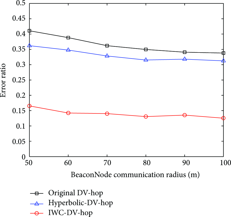
Comparison with different BeaconNode communication radii.

Comparison with different BeaconNode communication radii.
As what has been introduced above, the upper line shows the error ratio of original DV-hop algorithm varies with the increase of the communication radius, while the middle line shows the error ratio of hyperbolic-DV-hop algorithm and the lower line shows the error ratio of our IWC-DV-hop. We note that the accuracy is greatly improved by IWC-DV-hop, and the hyperbolic algorithm also works better than the original DV-hop. According to our records, the accuracy improvement of our hyperbolic-DV-hop over the original DV-hop is 9.3%, while our IWC-DV-hop over the original DV-hop is 62%.
Figure 7 indicates that, in general, the accuracy of our IWC-DV-hop is much better than Jian Li's WDV-hop algorithm and Bingjiao Zhang's WCL algorithm. It is worth mentioning that Jian Li's algorithm has better accuracy than our hyperbolic-DV-hop algorithm when the BeaconNode communication radius is larger than 60 m, but our hyperbolic-DV-hop algorithm performs better in those environments, the communication radius is small. We can conclude that the change in BeaconNode communication radius had minimal impact on performance, which means our two proposed algorithms have better stability.
6. Conclusions
Localization problem is one of the most important and different problems for WSNs. After a detailed study of positioning problem of wireless sensor network node location, two refined distance vector-hop (DV-hop) localization algorithms, hyperbolic-DV-hop localization algorithm and IWC-DV-hop localization algorithm, are proposed in this paper. Compared to the original DV-hop algorithm, the accuracy is improved by both algorithms, between which IWC-DV-hop performs even better. Our hyperbolic-DV-hop algorithm provides better accuracy than the original DV-hop algorithm because it chooses the average of average HopSizes of all BeaconNodes as the average HopSize of the UnknownNode instead of taking the average HopSize of BeaconNode nearest to the UnknownNode. It also replaces the ML localization algorithm with hyperbolic location algorithm with better performance results. Our IWC-DV-hop algorithm improves the accuracy by selecting appropriate BeaconNodes and replacing ML localization with centroid localization. A weight scheme has also been proposed to improve the accuracy by taking the influence of different BeaconNodes into consideration. Then we run simulations to compare the performance of different localization algorithms with different parameters. The results of simulations show that both our hyperbolic-DV-hop algorithm and IWC-DV-hop are much better than DV-hop localization algorithm. In addition, comparing to other localization algorithms for WSNs or other refined algorithms based on DV-hop, our IWC-DV still performs excellently. According to our simulations, our IWC-DV algorithm not only has a much better precision but also performs much more steadily no matter how the parameters change.
In the future, we will be interested in refining our localization algorithms even further and try to use it in the 3D situations. Some test-bed can also be constructed to allow us to compare real results with those simulation results.
Footnotes
Conflict of Interests
The authors declare that there is no conflict of interests regarding the publication of this paper.
Acknowledgments
This work is supported by National Training Program of Innovation and Entrepreneurship for Undergraduates (201410058046), National Nature Science Foundation of China (61272006), and Tianjin Higher Education Fund for Science and Technology Development under Grant no. 20110808.