Sage Journals: Discover world-class research

Abstract

Detecting abnormal events in multimedia sensor networks (MSNs) plays an increasingly essential role in our lives. Once video cameras cannot work (e.g., the sightline is blocked), audio sensor can provide us with critical information (e.g., in detecting the sound of gun-shot in the rainforest or the sound of car accident on a busy road). Audio sensors also have price advantage. Detecting abnormal audio events in complicated background environment is a very difficult problem; only few previous researches could offer good solution. In this paper, we proposed a novel method to detect the unexpected audio elements in multimedia sensor networks. Firstly, we collect enough normal audio elements and then use statistical learning method to train them offline. On the basis of these models, we establish a background pool by prior knowledge. The background pool contains expected audio effects. Finally, we decide whether an audio event is unexpected by comparing it with the background pool. In this way, we reduce the complexity of online training while ensuring the detection accuracy. We designed some experiments to verify the effectiveness of the proposed method. In conclusion, the experiments show that the proposed algorithm can achieve satisfying results.

1. Introduction

Nowadays, multimedia sensor networks (MSNs) become increasingly popular and important in our everyday lives [1, 2]. We can detect traffic accidents on a bustling road or wild hunting in rainforest by deploying video cameras or audio sensors.

Most monitoring systems utilize video cameras to detect abnormal events such as traffic accident or fire in forest [3]. However, video cameras cannot work well in some special situations, especially without sufficient light or when the sightline is blocked. Under these circumstances, audio sensors can provide us with sufficient information to make up for the lack of video sensors. It is becoming increasingly critical to use audio sensors to improve the effectiveness for monitoring systems, especially when video cameras cannot work effectively (e.g., the sightline is blocked). Audio sensors also have price advantage. Our research aims to utilize the acoustic clues as complementary information to automatically discover and analyze abnormal situations. Our goal is to make full use of audio cues, so as to access accurate detection and analysis of abnormal events.

Audio based surveillance system has been studied for many years. In [4] the authors designed a novel method to detect human coughing in the office. In [5], the authors used a SVM-based method to build an office monitoring system. This system can detect some impulsive sound such as door alarm and crying. In [6], the authors designed a HMM-based method to detect some special audio elements such as gun-shot and car-crashing. However, in some special monitoring systems (e.g., in the forest monitoring system), there is no need to distinguish gun-shot from animal scream; it is necessary to judge whether the event is expected to happen at a specific time and a specific location. Only few researches paid attention to define the background sounds and use them to detect some target audio effects [7, 8]. However, these researches are usually designed for some relatively quiet environments, such as office buildings, and thus cannot be directly used in noisy forest environment.

In summary, in order to detect abnormal audio events in complicated environment, it is critical to build a very large model for expected events, which require a large number of training samples and a considerable amount of computing power consumption. In this paper, we establish a comprehensive background pool to cover all the expected sounds. And then, we decide whether an audio event is unexpected by comparing it with the background pool. In order to get the model of the background pool, we first collect enough training samples for each expected audio effect and train them separately by using HMM. By doing so, we set the transition probabilities between these expected audio effects by some prior knowledge. By this way, we have established a hierarchical model, background pool model, to detect the unexpected audio effect. The advantage of this approach lies in the fact that we can reduce the costs of online training through training each basic audio effect model offline. In all, this method has better flexibility and scalability; that is, when the monitoring environment changes, there is no need to retrain the background model; we only need to add some new basic models into the background pool or remove some from the pool.

The rest of this paper is organized as follows. In Section 2, we describe the system architecture briefly. Section 3 presents the feature extraction method. In Section 4, we introduce how to build the model of the background pool. In Section 5, we present the abnormal event detection process. In Section 6, we show the experimental results. In the end, we conclude the paper and discuss the future works in Section 7.

2. Framework Overview

As is shown in Figure 1, the abnormal event detection system can be divided into two important parts, offline training process and online testing process. In the offline training process, we first collect enough training samples for each expected audio element and use HMM to train them offline. And then, the relationship among basic audio elements is determined by prior knowledge. In the online testing process, the audio sensor nodes capture the environmental information and extract the audio features. And then similarity degree between the audio signal and the background pool is calculated by the Viterbi algorithm. Finally, the cluster head fuses the information in its cluster and makes final decision.

Figure 1

The architecture of the abnormal event detection system.

3. Feature Extraction

Feature extraction plays a fundamental but essential role in pattern recognition, which determines the accuracy of the recognition results directly. Many audio features have been effective in previous research on audio classification [9, 10], for example, short-term energy and short-time zero-crossing rate. Since it can simulate human auditory system, mel-frequency cepstral coefficients (MFCCs) have been widely used in audio classification system in recent years. As is suggested in [11], eight-order mel-frequency cepstral coefficients (MFCCs) are selected for the proposed method. MFCCs are the mathematical coefficients for MFC and can be extracted as follows.

Step 1 (frame blocking).

In this step, we blocked the continuous audio signal into several frames; each frame is composed of N samples. The adjacent frames have T overlapping samples. Obviously, $T < N$ . According to some previous research, we set $N = 256$ and $T = 100$ .

Step 2 (windowing).

In this step, we reduce the discontinuities in the junction of two frames by windowing. Suppose defining $x (n)$ as the original signal for each audio frame, $w (n)$ is the window function, and the signal for each frame after windowing is as follows:

\begin{matrix} y (n) = x (n) w (n), 0 \leq n \leq N - 1 . \end{matrix}

(1)

Step 3 (fast Fourier transform).

In this step, we carry out a fast Fourier transform on the signal after windowing. That is to say, we convert the frames from the time domain to the frequency domain. The signal after fast Fourier transform is as follows:

\begin{matrix} Y_{n} = \sum_{k = 0}^{N - 1} y_{k} e^{- 2 π j k n / N}, n = 0,1, 2, \dots, N - 1 . \end{matrix}

(2)

Step 4 (mel-frequency wrapping).

In this step, we simulate the human auditory system by a filter bank. As is shown in Figure 2, the filter bank has a triangular band-pass frequency response, and the spacing is determined by a constant mel-frequency interval. Suppose that the number of mel spectrum coefficients is K, and according to previous research we set $K = 20$ .

Figure 2

The MFCCs extraction process.

Step 5 (discrete cosine transform).

In this step, we convert the log mel spectrum from the frequency domain back to the time domain (MFCC) using the discrete cosine transform (DCT). We denote the mel power spectrum coefficients to be the result of the last step $S_{k}$ , $k = 1,2, \dots, K$ , and then the MFCC's ( $c_{n}$ ) can be calculated as follows:

\begin{matrix} c = \sum_{k = 1}^{K} \log S_{k} \cos [n (k - \frac{1}{2}) \frac{π}{K}] . \end{matrix}

(3)

4. Background Pool Modeling

In the complicated monitoring environment, multiple audio elements may occur at the same time. How to build models is an important issue in detecting abnormal audio events. It is rather easy to use ICA (Independent Component Analysis) to separate different types of audio effects as in some controlled environment, such as movies. However, when it comes to the real scene, such as in a noisy rainforest, it is difficult to do so. What is more, because millions of data are required, building a huge model is so difficult that people have rarely achieved satisfying results based on that up to now. As a result, a background pool has been built, in which we train the basic effects, respectively, so as to observe the expected event. And then, we set transition probabilities among these elements according to some specific rules. This solution can help us effectively train those elements separately. In addition, this method has better flexibility and scalability. That is to say, although the monitoring environment changes, there is no need to retrain the background model; what is needed is to add some new basic models into the background pool or remove some from the pool; no extra training is needed.

4.1. Basic Audio Element Modeling

As is known to all, many previous researches on audio classification have been done to prove the effectiveness of Hidden Markov Model (HMM) [6, 9]. In this paper, we utilize HMM to train the signal audio effects. The model for ith basic audio element ( $B E_{i}$ ) in the background pool is defined as follows:

\begin{matrix} H_{i} = (S_{i}, V_{i}, A_{i}, B_{i}, Π_{i}) . \end{matrix}

(4)

(i)

$S_{i}$ is the state set, $S_{i} = {S_{i 1}, S_{i 2}, \dots, S_{i N_{i}}}$ , where $N_{i}$ stands for the number of states in ith basic element model ( $B E_{i}$ ).

(ii)

$V_{i}$ is the possible observed results for ith basic element model ( $B E_{i}$ ), $V_{i} = {V_{i 1}, V_{i 2}, \dots, V_{i M_{i}}}$ , and $M_{i}$ denotes the number of distinct observation symbols.

(iii)

$A_{i}$ is the transition probability distribution matrix between the states.

(iv)

$B_{i}$ is the observation probability distribution matrix for ith model.

(v)

$Π_{i}$ is the initial state probability vector. According to some previous works [6], the initial state probabilities are set to be equal; that is,

\begin{matrix} P (S_{i 1}) = P (S_{i 2}) = \dots = P (S_{i N_{i}}) = \frac{1}{N_{i}} . \end{matrix}

(5)

How to set the number of hidden states in the models directly determines the detection accuracy. On the one hand, the model states should be sufficient to describe acoustical characteristics. On the other hand, a large number of states may increase the complexity of the training and testing process. In this paper, we did a large number of experiments to balance the energy consumption and the detection accuracy and then set an appropriate model size for each basic audio element.

In this paper, we apply our proposed method to the noisy forest monitoring system, where 9 basic audio effects are collected to represent the background sound in the forest environment, namely, the crying of animals, chirping of insect, sound of water, sound of wind, sound of rain, sound of footstep, sound of inciting wings, and other backgrounds. The model size of each basic element is shown in Table 1. The result is reasonable because a large number of experiments are used to verify its effectiveness.

Table 1

The model size for the 9 chosen basic audio elements.

Basic audio element	Number of states
Crying of animals	3
Crying of birds	3
Chirping of insects	3
Sound of water	4
Sound of wind	3
Sound of rain	6
Sound of footstep	3
Sound of inciting wings	4
Other noises	3

For each basic audio element, we collect about 50–70 short clips as the training samples. We extract the MFCCs for each audio clip, and then the extracted MFCCs vectors are used as the input observations for the HMMs. According to some previous works [6], the Baum-Welch algorithm is then applied to estimate the transition probabilities between states and the observation probabilities in each state. After that, we have built the model for each basic audio element.

4.2. Background Pool Model

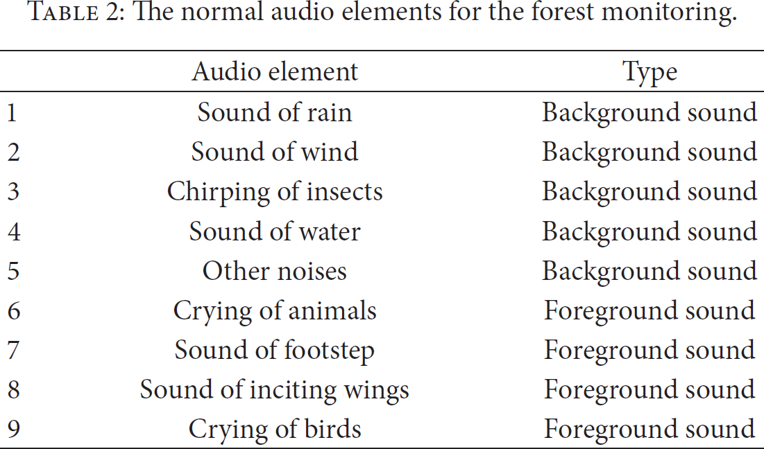
As is described above, the background pool is composed of several expected basic audio elements. For instance, in the forest environment, the background is often composed of the sound of rain, footstep, inciting wings, and so on. In many previous researches, researchers divided the audio signal into foreground sound and background sound. In this paper, we consider the basic audio elements that usually occur as the background sound and the audio elements that seldom occur as the foreground sound. For instance, in the forest environment, the sound of wind and water usually occurs, while the crying of animal rarely appears. We introduce a background pool to store all of the expected audio elements, and the background pool consists of the background sound and the foreground sound. The background pool will change in accordance with different monitoring environments.

For a given background pool P, let F be the set of foreground elements and let B be the set of background elements:

\begin{matrix} F = \{B E_{F 1}, B E_{F 1}, \dots, B E_{F N}\}, \\ B = \{B E_{B 1}, B E_{B 1}, \dots, B E_{B N}\}, \end{matrix}

(6)

where

B E_{F i}

is ith audio element in the foreground set and

B E_{B j}

is jth audio element in the background set. We have

\begin{matrix} F \cap B = ⌀ . \end{matrix}

(7)

Then, the background pool model is defined as follows:

\begin{matrix} P = (F, B, E), \end{matrix}

(8)

where

E = {〈B E_{i}, B E_{j}〉 | B E_{i}, B E_{j} \in F \cup B and p_{i j}}

, where

p_{i j}

is the transition probability from

B E_{i}

B E_{j}

. Then, we will discuss how to get the value

p_{i j}

in detail.

In the forest monitor system, we built a background pool based on 9 basic elements (see Table 2).

Table 2

The normal audio elements for the forest monitoring.

	Audio element	Type
1	Sound of rain	Background sound
2	Sound of wind	Background sound
3	Chirping of insects	Background sound
4	Sound of water	Background sound
5	Other noises	Background sound
6	Crying of animals	Foreground sound
7	Sound of footstep	Foreground sound
8	Sound of inciting wings	Foreground sound
9	Crying of birds	Foreground sound

We assume the following: (1)

An element in the background set can transfer to other background elements and the elements in the foreground set.

(2)

An element in the foreground set can only transfer to itself and the elements in the background.

Given a basic audio element 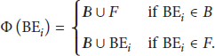$B E_{i}$ , we define its subsequent set, $Φ (B E_{i})$ , as a set of all the basic audio elements which $B E_{i}$ can transfer to; that is,

\begin{matrix} Φ (B E_{i}) = \{\begin{cases} B \cup F & if B E_{i} \in B \\ B \cup B E_{i} & if B E_{i} \in F . \end{cases} \end{matrix}

(9)

In order to reduce the complexity of training the transition probabilities, for a given basic audio element $B E_{i}$ , $\forall B E_{j} \in Φ (B E_{i})$ , the transition probability from $B E_{i}$ to $B E_{j}$ can be set as follows:

\begin{matrix} p_{i j} = \{\begin{cases} \frac{1}{|Φ (B E_{i})|} & if B E_{j} \in B \\ \frac{1}{|Φ (B E_{i})| \cdot |F \cup B|} & if B E_{j} \in F . \end{cases} \end{matrix}

(10)

In the end, we connect the audio effect models by some specific rules to build the model for the background pool.

5. Abnormal Audio Event Detection

In the online testing stage, each sensor collects audio signal in its own perception area. Firstly, the basic audio features energy and zero-crossing rate are extracted to analyze whether it is silent. If it is not a silent clip, the audio clip will be estimated by the background pool set; thus the log-likelihood value will be calculated. According to previous research, we use the Viterbi algorithm to compute the similarity of each audio clip and the background pool. Then each sensor transmits the current log-likelihood value to the cluster head.

Consider a cluster with N sensor node. The cluster head will fuse the collected information in its cluster as follows:

\begin{matrix} f = \sum_{i = 1}^{N} α_{i} \cdot s_{i}, \end{matrix}

(11)

where

s_{i}

denotes the log-likelihood value transmitted from ith audio sensor node and

α_{i}

is the weight of ith audio sensor. Obviously, the weight of each sensor node is determined jointly by many factors such as the distance from the key location, satisfying

\begin{matrix} \sum_{k = 1}^{N} α_{k} = 1 . \end{matrix}

(12)

In this paper, we set the weight value according to the instant short-term energy and the average short-term energy for each audio sensor node. Suppose that $E_{i I}$ denotes the instant short-term energy for ith audio sensor and $E_{k A}$ denotes the average short-term energy for ith audio sensor; then the relative energy change rate can be gained as follows:

\begin{matrix} R_{i} = \frac{|E_{i I} - E_{i A}|}{E_{i A}} . \end{matrix}

(13)

Generally, the closer ith node is apart from the instant audio event, the higher $R_{i}$ will be got. In this paper, the average short-term energy is regularly updated.

The weight value of the ith can be got as follows:

\begin{matrix} w_{i} = \frac{R_{i}}{\sum_{k = 1}^{n} R_{k}} . \end{matrix}

(14)

And then we will discuss how to determine whether there is an abnormal event based on the fused log-likelihood. In some previous research, researchers set a threshold to detect the abnormal event. That is to say, when the similarity between an audio clip and the background pool set gets close, the audio clip will be considered as normal sound, and vice versa. However, in the complicated environment monitoring, the background changes from time to time; thus it is hard to determine a threshold to adapt to dynamic monitoring requirements. Moreover, in monitoring systems, different missed detection will lead to different risk. Based on the above analysis, we make the final conclusion based on the minimum risk Bayesian decision theory.

Let x be observed audio clip; f is the fused log-likelihood value; we define the following:

$w_{1}$ : x is a normal audio event.

$w_{2}$ : x is an abnormal audio event.

$α_{1}$ : make the decision that x is a normal audio event.

$α_{2}$ : make the decision that x is an abnormal audio event.

Let $λ (j, k)$ be the risk factor for making the decision of $α_{k}$ while the fact is $w_{j}$ . In this paper, we define the risk decision ratio as $R = λ (1,2) : λ (2,1)$ , and this value should be set through a lot of experiments.

Then, we calculate the risk value for making the decisions $α_{1}$ and $α_{2}$ , respectively, according to [8]. Suppose that $R_{1}$ denotes the risk for making the decision $α_{1}$ and $R_{2}$ denotes the risk for making the decision $α_{2}$ . Then we make the conclusion as follows: (i)

The current audio clip is normal if $R_{1} / R_{2} \leq 1 .$

(ii)

The current audio clip is abnormal if $R_{1} / R_{2} > 1$ .

6. Experiments

In order to evaluate the performance of the proposed method, we deploy the algorithm in an audio wireless sensor network. As is shown in Figure 3, the selected cluster has 8 sensor nodes and one cluster head. In the experiment, we use a PC as the cluster head and the nodes transmit messages through the ZigBee wireless communication protocol.

Figure 3

The structure for a selected cluster in the audio sensor network.

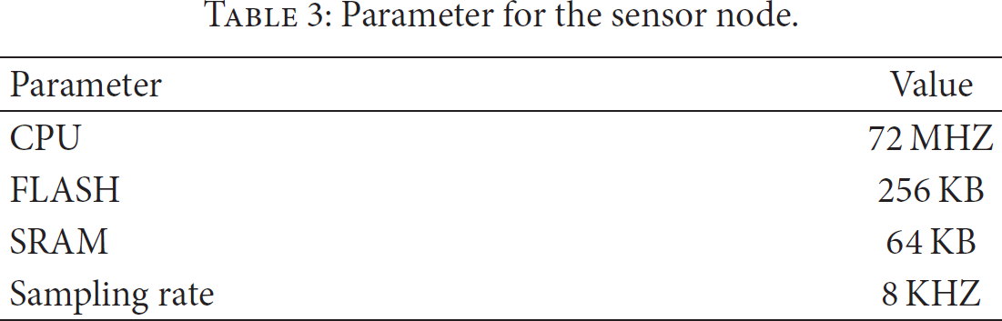
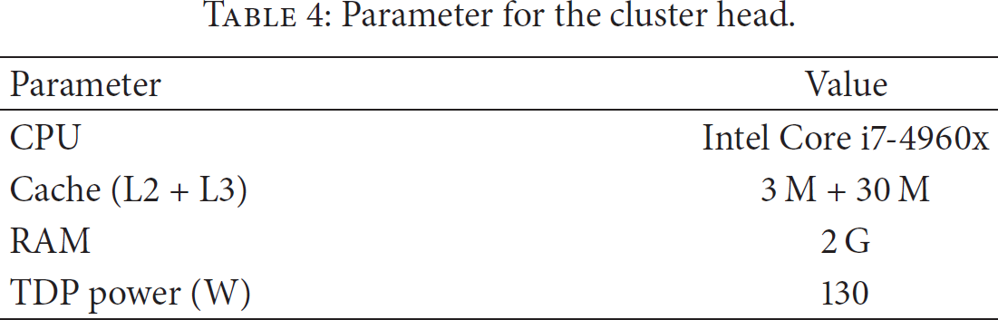
The detailed parameters of the sensor nodes and the cluster head are described in Tables 3 and 4.

Table 3

Parameter for the sensor node.

Parameter	Value
CPU	72 MHZ
FLASH	256 KB
SRAM	64 KB
Sampling rate	8 KHZ

Table 4

Parameter for the cluster head.

Parameter	Value
CPU	Intel Core i7-4960x
Cache (L2 + L3)	3 M + 30 M
RAM	2 G
TDP power (W)	130

6.1. Evaluation of the Background Pool Model

In this section, we choose 4 different types of abnormal audio elements to evaluate the performance of the background pool model (BGP), namely, engine, animal screams, gun-shot, and tapping sound of sticks. The expected data are collected from some documentary films such as “Animal Legend,” “Animal World,” and “Wonderful Broadcasting: Battle for survival The Animals' Guide to Survival.” The abnormal data are collected from some documentary films and action movies. In this experiment, we compare the proposed method with both SVM-based method and HMM-based method. The SVM-based method is introduced in [5], and the Gaussian radial basis function is used as the kernel function. The HMM-based method is introduced in [6], which has been widely used in creating keywords thus to be retrieved in movies. According to [6], the state number for each abnormal audio is set in Table 5.

Table 5

The model size for the 4 chosen abnormal audio events.

Basic audio element	Number of states
Engine	5
Animal screams	3
Gun-shot	3
Tapping sound of sticks	4

For each target abnormal audio event, we use the precision and recall to evaluate its detection accuracy:

\begin{matrix} precision = \frac{n_{c}}{n_{r}}, \\ recall = \frac{n_{c}}{n_{t}}, \end{matrix}

(15)

where

n_{c}

represent the number of audio frames detected correctly,

n_{r}

represents the number of all the audio frames determined as the specified audio type, and

n_{t}

is the total number of frames for the specified audio type in truth. The experiment results are shown in Figure 4.

Figure 4

The detection accuracy for three methods.

From Figure 4, we can see that, because of the complexity of the noisy forest monitoring environments, most previous works need a large number of training samples to ensure the accuracy of the detection. When the number of training samples reduces, the detection accuracy for HMM-based method and the SVM-based method reduces dramatically. By using the proposed background, we can reduce the complexity of the online training while ensuring the detection accuracy. In addition, this method has better flexibility and scalability. That is, when the monitoring environment changes, we do not need to retrain the background model; we only need to add some new basic models to the background pool or remove some from the pool.

6.2. Evaluation of the Decision Algorithm

As described in Section 5, how to set the risk decision ratio is very important in detecting the abnormal event, which directly determines the detection accuracy. In the experiments, we choose 4 different types of abnormal audio elements to choose the suitable risk decision ratio; they are engine, animal screams, gun-shot, and tapping sound of sticks. Then, we change the risk decision ratio R from 1 to 30 to show how the value affects the detection results (when $R = 1$ , the Bayesian-base method is equal to the threshold based method).

We can see in Figure 5 that as the risk decision ratio grows from 1 to 20, the detection recall is obviously increased. The reason lies in the fact that in the complicated monitoring environment several audio elements may occur at the same time; abnormal audio elements are usually mixed into the background noise. Take the sound of gun-shot, for example; since the duration of gun-shot is very short, the sampling window containing the sound of gun-shot may consist of at least two types of audio elements. By using the threshold based method, the sampling window is easy to be considered as other audio elements, while, by using Bayesian decision based method, we significantly improve the detection recall for abnormal audio events. However, when the risk decision ratio increases to a certain extent, the improvement of the recall is not obvious. In addition, the increase of the risk decision ratio will also affect the detection precision, especially when the value ranges to more than 25. We can see that better detection accuracy could be accessed when the risk decision ratio is set ranging from 10 to 20.

Figure 5

The evaluation of the risk decision ratio.

6.3. Evaluation of the Flexibility and the Scalability

In order to detect the abnormal audio events, there are two most common methods, modeling for the normal environment or modeling for the abnormal audio events. Then we compare the proposed method with these two methods when the monitoring environment or the monitoring tasks change. The comparing results are shown in Table 6.

Table 6

The comparison of the three methods when the monitoring environment or the monitoring tasks change.

	Environment changes	Abnormal events change
Environment-modeling	(i) Collecting enough samples and retraining the background model (ii) Need for a lot of time to collect the training samples (iii) The model is hard to converge in the complex environment	No extra work

Abnormal-modeling	No extra work	(i) Collecting enough samples and training models for the abnormal audio events (ii) Difficulty in dealing with the unexpected abnormal events

Our method	(i) Adding some new basic models to the background pool or removing some from the pool (ii) Changing the transition probabilities (iii) No extra training is needed	No extra work

When the background changes, environment-modeling method needs to collect enough samples and retain the background model to achieve satisfying detection accuracy; it will waste a lot of time. What is more, when the environment is complex, the model is very difficult to converge. By using the proposed method, only the transition probabilities need to be redefined, without any extra system retraining.

When the abnormal events change, abnormal-modeling method needs to collect enough samples for the abnormal audio events. The detection accuracy relies on the completeness of training samples. However, it is difficult to collect enough samples for the unexpected abnormal events in a short time. The proposed method will not be affected by this change.

7. Conclusions

In this paper, we propose a novel method to detect the abnormal audio event for complicated environment monitoring by using audio sensor networks. Firstly, we collect enough normal audio elements and use statistical learning method to train them offline. On the basis of these models, we establish a background pool by prior knowledge. The background pool contains expected audio effects. Finally we decide whether an audio event is unexpected by comparing it with the background pool. In this way, we reduce the complexity of the online training while ensuring the detection accuracy. We designed some experiments to verify the effectiveness of the proposed method, and the experiments show that the proposed algorithm can work well in the complex monitoring system.

Footnotes

Conflict of Interests

The authors declare that there is no conflict of interests regarding the publication of this paper.

Acknowledgment

This work is supported by the National Natural Science Foundation of China (Grant no. 61302087).

References

Apostolopoulos

J. G.

Chou

P. A.

Culbertson

Kalker

Trott

M. D.

Wee

The road to immersive communication

IEEE Journals & Magazines 2014 100 4 974 990

Edwar Murti

M. A.

Implementation and analysis of remote sensing payload nanosattelite for deforestation monitoring in Indonesian forest

Proceedings of the 6th International Conference on Recent Advances in Space Technologies (RAST '13)

June 2013

Istanbul, Turkey

IEEE

185 189

10.1109/rast.2013.6581197

2-s2.0-84883875861

Naikal

Yang

A. Y.

Sastry

S. S.

Towards an efficient distributed object recognition system in wireless smart camera networks

Proceedings of the 13th Conference on Information Fusion (Fusion '10)

July 2010

1 8

2-s2.0-79952420431

Cobos

Perez-Solano

J. J.

Felici-Castell

Segura

Navarro

J. M.

Cumulative-sum-based localization of sound events in low-cost wireless acoustic sensor networks

IEEE/ACM Transactions on Speech and Language Processing 2014 22 12 1792 1802

10.1109/taslp.2014.2351132

2-s2.0-84921822883

Kucukbay

S. E.

Sert

Audio-based event detection in office live environments using optimized MFCC-SVM approach

Proceedings of the IEEE International Conference on Semantic Computing (ICSC '15)

Feburary 2015

Anaheim, Calif, USA

475 480

10.1109/icosc.2015.7050855

Sandhan

Sonowal

Choi

J. Y.

Audio bank: a high-level acoustic signal representation for audio event recognition

Proceedings of the 14th International Conference on Control, Automation and Systems (ICCAS '14)

October 2014

Seoul, Republic of Korea

IEEE

82 87

10.1109/iccas.2014.6987963

2-s2.0-84920141312

Malik

Acoustic environment identification and its applications to audio forensics

IEEE Transactions on Information Forensics and Security 2013 8 11 1827 1837

10.1109/TIFS.2013.2280888

2-s2.0-84887057930

Choi

Rho

Han

D. K.

Selective background adaptation based abnormal acoustic event recognition for audio surveillance

Proceedings of the IEEE 9th International Conference on Advanced Video and Signal-Based Surveillance (AVSS '12)

September 2012

118 123

10.1109/avss.2012.65

2-s2.0-84868230248

Kolozali

Ş.

Barthet

Fazekas

Sandler

Automatic ontology generation for musical instruments based on audio analysis

IEEE Transactions on Audio, Speech and Language Processing 2013 21 10 2201 2220

10.1109/tasl.2013.2263801

2-s2.0-84881100438

10.

Umapathy

Krishnan

Jimaa

Multigroup classification of audio signals using time-frequency parameters

IEEE Transactions on Multimedia 2005 7 2 308 315

10.1109/tmm.2005.843363

2-s2.0-16244420091

11.

Henriquez

Alonso

J. B.

Ferrer

M. A.

Travieso

C. M.

Review of automatic fault diagnosis systems using audio and vibration signals

IEEE Transactions on Systems, Man, and Cybernetics: Systems 2014 44 5 642 652

10.1109/TSMCC.2013.2257752

2-s2.0-84899744851

Abnormal Event Detection Method in Multimedia Sensor Networks

Abstract

1. Introduction

2. Framework Overview

3. Feature Extraction

Step 1 (frame blocking).

Step 2 (windowing).

Step 3 (fast Fourier transform).

Step 4 (mel-frequency wrapping).

Step 5 (discrete cosine transform).

4. Background Pool Modeling

4.1. Basic Audio Element Modeling

4.2. Background Pool Model

5. Abnormal Audio Event Detection

6. Experiments

6.1. Evaluation of the Background Pool Model

6.2. Evaluation of the Decision Algorithm

6.3. Evaluation of the Flexibility and the Scalability

7. Conclusions

Footnotes

Conflict of Interests

Acknowledgment

References