Delay and Lifetime Performance of Underwater Wireless Sensor Networks with Mobile Element Based Data Collection

Abstract

Underwater Wireless Sensor Networks (UWSNs) may be easily partitioned due to resource constraints and sparse deployment, and such UWSNs need to be treated as Delay/Disruption Tolerant Networks (DTN). The principal objective of DTN routing is to maximize the possibility of eventual data delivery, which can be achieved only at the cost of high energy consumption and/or increased message latency. The energy efficiency and network lifetime are more important than data collection latency for certain underwater applications. We consider energy-efficient data collection using mobile elements, which is suitable for long-term sensing applications that are not time-critical. Using different analytical models, we investigate energy efficiency, network lifetime, packet delivery ratio, and message latency in a mobility-assisted data collection framework for UWSNs. The analytical models are validated with the experimental setup developed using the NS-2 based Aqua-Sim simulator. The results demonstrate that the proposed framework shows superior performance in terms of energy efficiency, network lifetime, and packet delivery ratio at the cost of increased message latency. The analytical models for delay performance are compared to see that the polling model is more effective in modelling the mobility-assisted data collection framework for UWSNs and more flexible in implementing different service policies.

1. Introduction

An underwater sensor network is made up of a group of many autonomous sensor nodes and vehicles deployed underwater and networked via acoustic links, performing collaborating tasks. They enhance our ability to observe and predict the ocean by enabling many applications such as oceanographic data collection, pollution monitoring, offshore exploration, disaster prevention, assisted navigation, and tactical surveillance. The underlying physical layer technology used in UWSNs is acoustic communication, since electromagnetic waves and optical signals are unsuitable due to high attenuation and scattering, respectively, in the underwater environment. UWSNs differ significantly from terrestrial sensor networks in several aspects: low and distance-dependent bandwidth, high latency, node mobility, high error probability, frequency dependent transmission range, 3-dimensional space, and so on [1]. The available bandwidth is of the order of 10 kHz at a few kilometres and the propagation speed is only around 1500 m/s.

The high cost of deploying and/or redeploying underwater equipment makes the issue of energy saving/efficiency a critical one for UWSNs. Underwater sensors are expensive, partially because of their more complex transceivers, and the ocean area that needs to be sensed is quite large. Hence, UWSN deployment can be much sparser compared with terrestrial sensor networks. In addition, the network may be easily partitioned due to node mobility, harsh environment, sparse deployment, and resource constraints. Such networks may never have an end-to-end contemporaneous path and traditional routing protocols are not practical since packets will be dropped when no routes are available. Hence, sparse and/or disconnected UWSNs are to be treated as ICNs or DTNs, but the conventional multicopy DTN approaches are not suitable due to resource constraints.

Three approaches have been reported for data collection in Wireless Sensor Networks [2], and they can be used in UWSNs also: (i) base station approach which uses direct communication between the sensor node and the sink, (ii) ad hoc network which uses a multihop path from the source to the sink, and (iii) mobility-assisted approach which makes use of mobile elements and the store-carry-forward concept for data collection. The first approach provides fast delivery but suffers from reduced life time of sensors due to relatively high communication energy. The ad hoc multihop network reduces the transmit power requirement and achieves medium delay but suffers from the “hot spot” problem near the sink and necessitates an end-to-end contemporaneous path between the source and the sink. Identifying the opportunities and challenges associated with the use of mobility-assisted approach for application-oriented periodic data collection in the harsh underwater environment and quantifying the resulting change in network performance constitute the focus of this paper.

We investigate the effectiveness of the mobile sink (MS) based architecture for continuous monitoring and offline data collection in sparse underwater acoustic sensor networks. We consider delay-tolerant deep water applications and use static two-dimensional UWSNs for ocean bottom monitoring. Analytical models for evaluating message delay, sensor buffer occupancy, Packet Delivery Ratio, node energy consumption, and network lifetime are presented. Three different analytical models using queueing theoretic approaches are used to evaluate and predict the delay performance: bulk service queue, $\text{M}/\text{G}/\mathrm{1}$ queue with vacation, and polling. A comparison of these delay models and the validation/comparison of the analytical results with the simulation results are also presented. A significant contribution of our work is the development of an analytical model for network lifetime improvement factor achieved by employing mobility-assisted data collection in UWSNs, taking into account all the peculiarities of the underwater channel and propagation. Another major contribution is the identification of the appropriate delay model to be used, based on the service policy of the mobile sink, which, in turn depends on the requirements of the application. Yet another contribution is the investigation of the impact of MS trajectories on the network performance. The analytical models are validated using simulation models developed in Aqua-Sim [3], an NS-2 [4] based network simulator developed by the University of Connecticut. By incorporating the DTN concepts and polling schemes into Aqua-Sim, an improved NS-2 based simulation model for application-oriented and energy-efficient data collection in underwater environment is made available, which we hope will widen the facility for further research in this area.

The remainder of this paper is organized as follows: Section 2 summarizes the related work. Proposed MS-based data collection framework is presented in Section 3. Analytical models for node energy consumption, network lifetime and delay performance are presented in Section 4. Section 5 presents the analytical and simulation results, followed by a discussion and comparison of delay models in Section 6. Finally, the paper is concluded in Section 7.

2. Related Work

The main research challenges in this area are identified in [1], mainly concentrating on hardware and protocol issues and a cross-layer design approach is highly advocated in it. In spite of the significant work envisioning novel applications and high-level architectures, not much research has addressed the design of supporting communication and networking protocols. Most original contributions have focused on acoustic modem design. Recently, several routing protocols have been developed for underwater sensor networks, most of them suitable only for connected networks. A detailed review and comparison of different routing techniques for UWSNs is given in [5]. Vector-based forwarding (VBF) is a typical geographical routing protocol [6] and hop-by-hop vector-based forwarding (HH-VBF) [7] is its more energy-efficient version. Both VBF and HH-VBF take care of node mobility, but they require the network to be connected and the energy overhead is quite high. Distributed routing algorithms for delay-sensitive and delay-insensitive applications are proposed in [8]. Cui et al. [9] present the interesting paradigm of mobile UWSN, that is, networks where the underwater sensors move because of water currents. Two interesting architectures are investigated, one for long-term nontime-critical applications (e.g., oceanography and pollution detection) and the other for short-term time-critical explorations (e.g., disaster prevention and military surveillance). Energy analysis of routing protocols for UWSNs is presented in [10] and energy-efficient routing schemes for UWSNs have been discussed in [11]. The key parameters that affect the lifetime of Wireless Sensor Networks have been identified in [12] and the use of AUVs to prolong lifetime in UWSN is discussed in [13].

Recently, considerable effort has been devoted to developing architectures and routing algorithms for DTNs [14, 15], characterized by frequent partitions and potentially long message delivery delays. A survey of routing in ICNs and DTNs is presented in [16]. Shah et al. [2] have presented a three-tier architecture based on mobility to address the problem of energy-efficient data collection in a terrestrial sensor network. For the same architecture, an enhanced analytical model has been presented in [17]. The current state-of-the-art solutions in underwater DTNs is presented in [18]. An adaptive routing protocol has been proposed in [19] for UWSN, considering it as a DTN. In order to increase the energy efficiency in resource constrained underwater environment, a delay-tolerant data dolphin (DDD) scheme is presented in [20]. A survey of data collection in Wireless Sensor Networks with mobile elements has been done in [21]. Use of Mobile Data Collectors (MDC) for reliable and energy-efficient data collection in sparse sensor networks is studied in [22]. A message ferrying approach for data delivery in sparse mobile ad hoc networks is presented in [23] and controlling the mobility of multiple data transport ferries in a DTN is discussed in [24]. The use of controllably mobile elements to reduce the energy consumption for communication and thus to increase useful network life time has been discussed in [25]. The usage of message ferries in ad hoc networks is considered in [26] and the design of message ferry route for sparse ad hoc networks with nodes having arbitrary movement is presented in [27]. AUV-aided routing for UWSNs is discussed in [28, 29], and the performance of DTN routing protocols for UWSNs is analyzed in [30].

To analytically evaluate the latency performance of data collection, the data collection process with a single mobile sink is modelled as an $\text{M}/\text{G}/\mathrm{1}$ queueing model in [31]. Polling-based scheduling with QoS capability for wireless body sensor networks is presented in [32]. Mobile element scheduling for data collection in terrestrial sensor networks is discussed in [33–35]. A rendezvous based approach with mobile sinks is used in [36] and rendezvous planning in sensor networks is investigated in [37]. The message ferrying DTN schemes and algorithms presented in [23, 24, 27] are found to be interesting and effective for successful data delivery in sparse networks with mobile nodes; however, their impact on network performance has not been properly quantified using analytical techniques.

Mobility-assisted on-demand data collection in sparse UWSNs is presented in our previous paper [38], which is aimed at supporting delay-sensitive event-driven applications in sparse UWSNs and makes use of a polling model for delay analysis. In contrast, the work presented in this paper is aimed at supporting energy-efficient off-line data collection scheme for periodic sensing applications in UWSNs, where network lifetime is more important than message delay. The existing literature on mobility-assisted data collection in UWSNs has focussed either on the aspects of energy efficiency and lifetime enhancement or on the aspects of message delay and successful delivery. We have adopted a comprehensive approach that considers all the aspects of data collection like energy efficiency, network lifetime, message latency, sensor buffer occupancy, and Packet Delivery Ratio of the proposed mobility-assisted data collection framework for delay-tolerant applications in sparse UWSNs. Three different analytical models are proposed to investigate the latency performance of the data collection scheme and the merits/demerits of each model, and the factors affecting their choice for a specified application are identified. To the best of our knowledge, there exists no other works in the literature, in which such a comprehensive approach for network performance evaluation is adopted and a comparison of delay models is made to identify the most suitable one to be adopted by the network designer, according to the resource constraints and application requirements.

3. System Model

The general UWSN scenario as shown in Figure 1 consists of a group of different kinds of sensor nodes and underwater vehicles used for collaborative monitoring. Depending on the application, either 3-dimensional or 2-dimensional node deployment is possible. In a 3D network, ordinary sensor nodes float at different depths and they can communicate using acoustic links. They relay data to the sinks using direct link or through multihop paths. In a 2D network, sensor nodes are anchored to the ocean bottom and are interconnected to one or more underwater sinks by means of wireless acoustic links. The sinks may be surface sinks or underwater sinks; the former can communicate with the command centre on shore or mother ship via RF links and with the underwater sensor nodes via acoustic link, while the latter is responsible for receiving data from the neighbouring nodes in the ocean bottom and relaying it to the surface sink. There will be mobile nodes with varying capabilities, ranging from courier nodes capable of moving in vertical direction alone to sophisticated Autonomous Underwater Vehicles (AUVs) with multiple underwater sensors and trajectory control mechanisms.

Figure 1

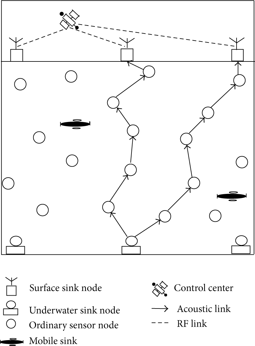
Underwater Wireless Sensor Network: general scenario.

The UWSNs considered in our study are large and mostly sparse, with possibly disconnected components and with mobile elements used for data collection. We consider 2-dimensional network with sensor nodes anchored to the ocean bottom and a mobile node used for data collection, a model of which is illustrated in Figure 2. The mobile node is assumed to be rechargeable or resource-unconstrained and hence its energy consumption for communication with underwater or surface sink is not considered. Since the underwater sink nodes can be equipped with optional high speed fibre optic link with the surface sink, and the surface sinks are equipped with RF links with the command centre, we restrict our study to the mobility-assisted data collection in the 2-dimensional ocean bottom area alone. In addition, data is assumed to be successfully delivered once it has been collected by the mobile sink. Therefore, aspects like the distribution of surface sinks, communication between mobile sink and underwater sink, communication between underwater sink and surface sink, and so forth are not considered. For the purpose of analyzing the network life time in ad hoc multihop scheme, we assume the network to be dense or connected, since the routing overhead can be best illustrated with such a network.

Figure 2

System model: 2D network for ocean bottom monitoring with MS for data collection.

3.1. Mobility-Assisted Data Collection

We consider a modified form of the 3-tier architecture [17] for mobility-assisted data collection, with the upper two layers merged together, resulting in a mobile sink (MS) architecture. The static sensors monitor the underwater surroundings, generate data, and store it in the sensor buffer until a contact or transmission opportunity occurs. They have limited battery power and buffer space and can communicate using acoustic links only. Their data communications are limited to single hop data transfer to a nearby mobile sink (MS), so as to reduce energy consumption.

Mobile sinks are mobile entities with large processing and storage capacity, renewable power, and the ability to communicate with static sensors and other sinks (if any). As an MS moves in close proximity to (i.e., within transmission range of) a static sensor, the sensor's data is transferred to the MS and buffered there for further processing. The MS can pause at the vicinity of the sensor till all the buffered data has been transferred. The mobility of the MS can be either random or controlled. In the case of random mobility, the worst-case latency of data transfer cannot be bounded. This unbounded latency may lead to excessive data caching and result in buffer overflows. Hence, it is better to use controlled mobility whenever it is feasible. If the MS is already deployed and its trajectory cannot be controlled (e.g., sensors attached to watery mammals), random mobility can be made use of, even though with reduced performance.

A sensor needs to detect a contact or the presence of a nearby MS to be able to send its data. In the proposed framework, the responsibility of contact discovery is with the MS and it periodically sends out HELLO messages to notify its presence. The amount of data collected in a single visit of the MS depends on the service policy and can be fixed according to the application requirements and network conditions. After collecting the data generated and buffered by the sensor node, the MS proceeds to the next location and this process is repeated. If the location information of the sensors with buffered data is known to the MS in advance, the MS may visit them in an optimum manner; otherwise, a trajectory that covers the deployment area is selected and both contact discovery and data transfer are carried out while moving along this trajectory.

3.1.1. MS Trajectories

Different MS trajectories, as shown in Figure 3, can be employed [28, 39, 40], keeping in mind that the basic application is periodic surveying of a region at sea. Some other possible trajectories (not shown in the figure) are circular, lawn-mower, and figure of eight [41]. Complex trajectories will be required for event-driven on-demand data collection, but here we consider simple cyclic paths suitable for periodic off line data collection for delay-tolerant applications. Trajectories B and C are similar, the difference being in the time to complete one cycle and the transmit power requirement of static sensors to ensure connectivity. E consists of three mobile sinks, each following a separate elliptical trajectory.

Figure 3

Controlled trajectories of MS.

The choice of a particular trajectory for a specific application depends on the application requirements, position of underwater sink, and energy constraints of nodes. Trajectories A and D with large travel time of MS are expected to be suited for delay-tolerant applications, whereas C and E with less travel times may be suitable for delay-sensitive applications. B, C, and D fit well for a scenario in which the UW sink is located at the centre, while E is specially suited for the sink located at the middle of one side of the square deployment area. We restrict our study to the first three trajectories alone, because of our assumption of a single MS in the system model, and the practical difficulty in guiding the MS along a cyclic spiral path on the ocean bottom.

3.2. Performance Metrics

The important performance metrics for mobility-assisted data collection are Packet Delivery Ratio (PDR), message latency, node energy consumption, network lifetime, and buffer space requirement at sensors.

3.2.1. Packet Delivery Ratio

The effectiveness of data delivery is indicated by the PDR and it can be affected by errors in communication, buffer overflow, or failure of MS. If the MS does not approach the sensor for a long time, the buffer may fill up and eventually overflow, resulting in packet loss.

3.2.2. Message Latency

Latency is the average time taken by the data to reach the sink from the time of its generation. Since data is assumed to be successfully delivered once it has been collected by the MS, latency has only two components in our model: queueing delay in the sensor buffer and the service time for transferring the data from the sensor to the MS. Due to limited speed of the MS (maximum 20 m/s due to practical reasons), the travel time of the MS is expected to be very large (of the order of several minutes or even few hours for large networks).

3.2.3. Energy Consumption

Energy required for sensing is negligible compared to that for communication, and energy consumption for reception is very small compared to that for transmission. Assuming tunable transmit power, short range single hop communication between the static sensors and MS is expected to reduce and balance the energy consumption among sensors.

3.2.4. Network Lifetime

Network lifetime is the time span from the deployment to the instant when the network is considered nonfunctional: when a network should be considered nonfunctional is, however, application-specific [12]. It has been defined in many ways by different researchers [42]. Network lifetime is a key characteristic to evaluate the performance of sensor networks and parameters like coverage, connectivity, and node availability can be reduced to lifetime considerations. Reduced and balanced energy consumption among the nodes will lead to enhanced network lifetime in MS-based architecture.

3.2.5. Sensor Buffer Occupancy

Since the generated packets are to be stored in the sensor buffer till the arrival of the MS, buffer capacity should be sufficiently high to avoid buffer overflow and packet loss. Average buffer occupancy gives an indication about the buffer space to be allotted for a particular application depending on the data generation rate and the MS arrival rate.

4. Analytical Study

In this section, the energy consumption and lifetime of the sensor network as well as the latency and delivery ratio of the sensed data are investigated through analytical means. The average sensor buffer occupancy and the network lifetime improvement factor are also evaluated. All the features of acoustic propagation and devices significantly affect these performance measures and hence the performance of the data collection schemes. The study permits us to assess the impact of a set of network parameters like depth of deployment, target SNR, sensor power profile, data arrival rate, data transfer rate, sensor buffer size, number and range of sensor nodes, MS visit frequency, service discipline, MS movement pattern, and so forth on the performance metrics and hence to decide the appropriate values for these parameters according to specific application requirements.

4.1. Energy Consumption and Network Lifetime

Energy consumption needs to be considered as a critical issue since it is difficult to recharge or even replace batteries for a large number of sparsely distributed sensors. One important motivation for employing a mobile sink is that it increases the energy efficiency and lifetime of the network by reducing the source-destination distance and eliminating the relaying of data. We compare the energy consumption of static sensor nodes considering direct, multihop and MS-based data transmission schemes. Since multihop communication necessitates an end-to-end contemporaneous path between the source and sink, we assume the network to be connected (by deploying sufficiently large number of nodes or by increasing the transmission range of the nodes to ensure connectivity).

4.1.1. Hop Energy Consumption

The battery power required for sensing and processing is negligible compared to that for underwater acoustic data transmission, and hence we consider the energy consumption for data transmission only. Also, we assume that the sensor nodes have fixed receive power and tunable transmit power, that is, the transmit power can be varied according to the range of operation. We consider the effects of path loss and noise for our energy analysis, the two main sources of transmission losses being attenuation and spreading [10].

The propagation model helps us to estimate the transmit power required for a specified target signal-to-noise ratio (SNR). The SNR of an emitted underwater signal at the receiver is expressed by the passive sonar equation as [43]

$$\begin{array}{cc}& \text{SNR}=\text{SL}-\text{TL}\left(l,f\right)-\text{NL}\left(f\right)+\text{DI},\end{array}$$

(1)

where $\text{SL}$ is the source level, TL is the transmission loss which is a function of distance l and frequency of operation f, NL is the frequency-dependent noise level, and DI is the directivity index. The source level SL $=\mathrm{20}\log I$ , where I is the intensity at 1 m from the source (expressed in $\text{watts}/{\text{m}}^{\mathrm{2}}$ ) and is given by $I=P_t/\mathrm{2}\pi H$ , where $P_t$ is the transmit power and H is the water depth in metres. All quantities in (1) are in dB re μPa, where the reference value 1 μPa corresponds to the intensity value of $0.67\times \mathrm{1}{\mathrm{0}}^{-\mathrm{18}}$  W/m². Assuming a target SNR of 20 dB at the receiver, an ambient noise level of 70 dB (which is representative of underwater environments), and omnidirectional antennas for transmission and reception, we have the required source level:

$$\begin{array}{cc}& \text{SL}=\text{TL}+\mathrm{90}.\end{array}$$

(2)

Considering the effects of absorption and spreading, the transmission loss or the attenuation factor $\text{TL}(l,f)$ of an underwater acoustic channel for a distance l and frequency f is given by [43]

$$\begin{array}{cc}& \mathrm{10}\log \text{TL}\left(l,f\right)=k·\mathrm{10}\log l+l·\mathrm{10}\log a\left(f\right),\end{array}$$

(3)

where the first term is the spreading loss and the second term is the absorption loss. Spreading loss is independent of frequency and depends only on the geometry. The spreading coefficient $k=1$ for cylindrical spreading and $k=2$ for spherical case. The spreading is assumed to be cylindrical in shallow water and spherical in deep water; hence, the variation of spreading loss with distance is linear in shallow water, while it is quadratic in deep water. Absorption loss increases with frequency and the distance between nodes.

Thorp's formula [44] is used to express the absorption coefficient as

$$\begin{array}{cc}& \mathrm{10}\log a\left(f\right)=\frac{\mathrm{0.11}{f}^{\mathrm{2}}}{\mathrm{1}+f^{\mathrm{2}}}+\frac{\mathrm{44}{f}^{\mathrm{2}}}{\mathrm{4100}+f^{\mathrm{2}}}+\frac{\mathrm{2.75}{f}^{\mathrm{2}}}{\mathrm{1}{\mathrm{0}}^{\mathrm{4}}}+\mathrm{0.003}.\end{array}$$

(4)

If a tone of frequency f and power $P_t$ is transmitted over a distance l, the received signal power will be $P_t/\text{TL}(l,f)$ . For a given target signal-to-noise ratio $\text{SN}{\text{R}}_{tgt}$ , available channel bandwidth $B(l)$ , and noise power spectral density $N(f)$ , the required transmit power $P_t(l)$ can be expressed as a function of the transmitter-receiver distance l [11] as

$$\begin{array}{cc}& P_t\left(l\right)=\frac{\chi }{\xi }B\left(l\right)N\left(f\right)A\left(l,f\right){\text{SNR}}_{tgt},\end{array}$$

(5)

where χ is a margin to ensure that the average SNR at the receiver is larger than the minimum required value and ξ is a penalty factor that accounts for signal processing inefficiencies at the receiver. Acoustic power is converted to electrical power by the relation [43]:

$$\begin{array}{cc}& P_t^{\text{el}}=P_t\left(l\right)·\frac{\mathrm{1}{\mathrm{0}}^{-\mathrm{17.2}}}{\eta },\end{array}$$

(6)

where $\mathrm{1}{\mathrm{0}}^{-\mathrm{17.2}}$ is the conversion factor from acoustic power in dB re μPa to electrical power in Watts and η is the overall efficiency of the electronic circuitry [11]. The receive power $P_r$ is independent of distance and depends on the complexity of the receiver circuitry. If L is the packet size in bits and α is the bandwidth efficiency of modulation, the energy consumption for the transfer of a packet over a single hop of length l becomes

$$\begin{array}{cc}& E_{\text{hop}}\left(l\right)=\frac{\left(P_r+P_t^{\text{el}}\left(l\right)\right)L}{\alpha B\left(l\right)},\end{array}$$

(7)

where $P_t^{\text{el}}(l)$ is the electrical power (in watts) corresponding to $P_t(l)$ in dB re μPa.

Compared to $P_r$ , $P_t^{\text{el}}$ is very large and hence its contribution to the energy consumption of sensor nodes is significant. As the transmission loss is proportional to the square of the hop length in the deep water scenario, the energy consumption of sensor nodes can be reduced considerably by reducing the source to sink distance and/or increasing the channel bandwidth. Unlike terrestrial channels, underwater acoustic channel exhibits distance-dependant bandwidth, a few kHz in long range (several tens of kilometres) systems to more than hundred kHz in short-range (several tens of meters) systems. The very large transmit power requirement at large distances results in heavy energy consumption and increased level of interference. Hence, single hop (direct) data transmission is not feasible if source-to-destination distance is large and we will not consider the direct transmission (BS approach) further.

4.1.2. Relaying Overhead and Energy Efficiency

Assuming ideal channel with no packet errors, energy efficiency can be increased by reducing the relaying overhead. The important motivations for using a mobile element for data collection are as follows: (i) it eliminates the need for end-to-end connectivity between source and destination; (ii) it reduces energy consumption by reducing the transmission range; and (iii) it balances the energy consumption by eliminating the relaying of data. The first feature contributes to improved data delivery performance, and the other two features lead to enhanced lifetime of the network. To quantify the potential savings in energy consumption and network lifetime, we compare the energy requirements with and without a mobile node. The energy consumption of static nodes alone is considered, since the mobile node is assumed to be rechargeable or not energy-constrained.

Though we have considered a square deployment area in our system model, for tractability in the analysis of relaying overhead in ad hoc multihop network, we approximate it by a circular area whose diameter equals the side of the square. Assume N static sensor nodes to be randomly deployed with uniform distribution over a circular area A of radius R. Unlike our earlier system model with sparse deployment of sensors, here we assume a sufficiently large value for N that results in a connected ad hoc multihop network, since the relaying overhead can be best illustrated with such a network. The static sensor nodes generate and send data to the sink, located at the centre of the circular area. We assume that an ideal Medium Access Control (MAC) is available so that no energy is wasted in collisions. To quantify the relaying overhead in the multihop ad hoc network, we follow the approach similar to the one used in [25] and consider the number of transmissions incurred by the nodes located at different distances from the sink.

Let the transmission range of the nodes be r. The circular deployment region is divided into concentric annuli to count the minimum number of relay hops required for each node to reach the sink. Since the nodes are uniformly distributed, the number of nodes in kth annular region of area $A(k)$ is approximately equal to $N(A(k)/A)$ for large N. If each static node in the kth annulus generates one message, then the minimum number of transmissions originated from the kth annulus is $\mathrm{Min}Tx(k)=N(A\left(k\right)/A)k$ .

Now each of these transmissions will be received by at least one node in the $(k-1)$ th annulus and transmitted towards the inner annulus. Hence, in the case of multihop architecture, if every node generates 1 packet, for a large value of N, on an average, the number of receptions and transmissions to be undertaken by a node in annulus k will be

$$\begin{array}{cc}& \text{Node}Rx\left(k\right)=\frac{A\left(k+\mathrm{1}\right)}{A\left(k\right)}\text{Node}Tx\left(k+\mathrm{1}\right),\end{array}$$

(8)

$$\begin{array}{cc}& \text{Node}Tx\left(k\right)=\mathrm{1}+\frac{A\left(k+\mathrm{1}\right)}{A\left(k\right)}\text{Node}Tx\left(k+\mathrm{1}\right),\end{array}$$

(9)

respectively, except for the outermost annulus where the corresponding values are 0 and 1. Hence, the energy consumed by a static node in the kth annulus ( $1\le k\le ⌈R/r⌉$ ) for the transfer of M packets of L bits each from each static sensor to the sink will be

$$\begin{array}{l}\text{NodeEnergy}\left(k\right)\\ =\text{ML}\frac{\left(P_r·\text{Node}Rx\left(k\right)+P_t\left(r\right)·\text{Node}Tx\left(k\right)\right)}{\alpha B\left(r\right)}.\end{array}$$

(10)

In the mobility-assisted data collection, irrespective of the position of the nodes, each static node transmits only the packets generated by it. Thus, the energy consumed by a static node for transferring M packets of L bits each becomes

$$\begin{array}{cc}& \text{NodeEnergy}=\text{ML}\frac{P_t\left(r\right)}{\alpha B\left(r\right)}\end{array}$$

(11)

which is independent of its proximity to the sink. If we define the Relaying Overhead Index(ROI) of a sensor node as the ratio of the total number of transmissions from the node to the number of transmissions corresponding to the packets originated at that node, it is evident that all the sensor nodes have the same ROI (equal to l with an error-free channel) in MS-based scheme, while it is approximately equal to $\text{Node}Tx(k)$ in multihop network. Since relaying is eliminated in MS-based scheme, total energy consumption is equally divided among all the N nodes, thus balancing the energy consumption.

4.1.3. Network Lifetime

Network lifetime forms an upper bound for the utility of the sensor network and it strongly depends on the lifetimes of the individual nodes that constitute the network [42].

We consider lifetime as the time until the first sensor node is drained off its energy and use the general formula for it as derived in [12] and restated as follows.

For a WSN with total nonrechargeable initial energy $E_{\mathrm{0}}$ , the average network lifetime $\mathbb{E}[\mathfrak{L}]$ , measured as the average amount of time until the network dies, is given by

$$\begin{array}{cc}& \mathbb{E}\left[\mathfrak{L}\right]=\frac{E_{\mathrm{0}}-\mathbb{E}\left[E_w\right]}{P_c+\mu \mathbb{E}\left[E_{\text{comm}}\right]},\end{array}$$

(12)

where $P_c$ is the constant continuous power consumption over the whole network, $\mathbb{E}[E_w]$ is the expected wasted energy (i.e., the total unused energy in the network when it dies), μ is the average sensor reporting rate, and $\mathbb{E}[E_{\text{comm}}]$ is the expected communication energy consumed by all sensors in a randomly chosen data collection.

If we ignore the idle time energy consumption in our network and define the network lifetime as the time span until the first death of any sensor, then

$$\begin{array}{cc}& \mathbb{E}\left[\mathfrak{L}\right]=\frac{E_{\mathrm{0}}-\mathbb{E}\left[E_w\right]}{\mu \mathbb{E}\left[E_{\text{comm}}\right]}.\end{array}$$

(13)

Hence, a lifetime-maximizing data collection scheme should aim at reducing the average wasted energy $\mathbb{E}[E_w]$ and the average communication energy $\mathbb{E}[E_{\text{comm}}]$ . Mobility-assisted data collection achieves balanced energy consumption (thus reducing the average wasted energy) and reduced communication energy, thus enhancing the network lifetime as given by (13).

The potential saving in network lifetime of MS-based model compared to the ad hoc multihop network can be quantified in terms of the relaying overhead of the nodes as derived in Section 4.1.2. If $E_i$ represents the initial energy of a static sensor, the lifetime of a node expressed in terms of the maximum number of original packet transmissions over a distance of length l that can be afforded by it, before being completely drained off its battery power, can be expressed as

$$\begin{array}{cc}& N_{\text{LMH}}\left(k\right)=\frac{E_i}{E_{\text{hop}}\left(l\right)\text{Node}Tx\left(k\right)},\end{array}$$

(14)

$$\begin{array}{cc}& N_{\text{LMS}}=\frac{E_i}{E_{\text{hop}}\left(l\right)}\text{\hspace{0.17em}\hspace{0.17em}and}\end{array}$$

(15)

for ad hoc multihop and MS-based data collection schemes, respectively. In (14) and (15), $E_{\text{hop}}(l)$ is given by (7) and $\text{Node}Tx(k)$ is given by (9).

Since the relaying overhead of a node in ad hoc multihop network (represented by $\text{Node}Tx(k)$ ) increases with its proximity to sink, (14) shows that the lifetime of a single node is maximum for the nodes in the periphery of the network and it decreases with proximity to sink. For MS-based scheme, the node lifetime as indicated by (15) is same for all static sensors irrespective of its location.

The network is considered dead if any of the sensors die due to energy depletion. Assuming the deployment area of sensor nodes to be very large compared to the transmission range (quite typical of UWSNs), single hop direct communication is infeasible, and the network lifetime in multihop network is limited by the relaying overhead of the single hop neighbours of the sink. Hence, in terms of number of transmissions, the network lifetime $\text{S}{\text{N}}_{\text{LMH}}$ and $\text{S}{\text{N}}_{\text{MS}}$ for multihop and MS-based schemes, respectively, can be expressed as

$$\begin{array}{l}\text{S}{\text{N}}_{\text{LMH}}\\ =\min \left\{N_{\text{LMH}}\left(\mathrm{1}\right),N_{\text{LMH}}\left(\mathrm{2}\right),\dots ,N_{\text{LMH}}\left(⌈\frac{R}{r}⌉\right)\right\},\\ \text{S}{\text{N}}_{\text{LMS}}=N_{\text{LMS}}.\end{array}$$

(16)

From (9) and (14),

$$\begin{array}{l}\min \left\{N_{\text{LMH}}\left(\mathrm{1}\right),N_{\text{LMH}}\left(\mathrm{2}\right),\dots ,N_{\text{LMH}}\left(⌈\frac{R}{r}⌉\right)\right\}\\ =N_{\text{LMH}}\left(\mathrm{1}\right).\end{array}$$

(17)

Hence, the lifetime improvement factor η of the proposed MS-based framework over the ad hoc multihop approach can be expressed as

$$\begin{array}{l}\eta =\frac{\text{S}{\text{N}}_{\text{LMS}}-\text{S}{\text{N}}_{\text{LMH}}}{\text{S}{\text{N}}_{\text{LMH}}}=\frac{N_{\text{LMS}}}{N_{\text{LMH}}\left(\mathrm{1}\right)}-\mathrm{1}\\ =\text{Node}Tx\left(\mathrm{1}\right)-\mathrm{1}.\end{array}$$

(18)

Thus, the lifetime improvement factor is the average number of transmissions to be undertaken by any of the 1-hop neighbours of the sink node, corresponding to a single packet transmission from each of the sensor nodes in the outer annuli. Using (9) and (18) can be simplified to obtain

$$\begin{array}{cc}& \eta =\frac{A\left(\mathrm{2}\right)+A\left(\mathrm{3}\right)+\cdots +A\left(⌈R/r⌉\right)}{A\left(\mathrm{1}\right)}=\frac{R^{\mathrm{2}}-r^{\mathrm{2}}}{r^{\mathrm{2}}}.\end{array}$$

(19)

Equation (19) shows that the relative improvement in lifetime is proportional to the ratio of area of the region outside one-hop neighbourhood of the sink located at the centre to that of the region within one-hop neighbourhood. It is evident from (19) that the network lifetime improvement is more pronounced in the case of large networks (high R) and with sensors having small transmit power or short range of transmission (r). Also, the lifetime improvement is independent of the traffic type, data generation rate, MS arrival rate, packet length, and channel bandwidth. The numerical results from this analytical model are compared with the simulation results in Section 5.

4.2. Latency and Buffer Occupancy

In the MS-based network model, packets generated at the static sensor nodes at random intervals are queued in the sensor buffer, waiting for a contact or transmission opportunity. When a contact occurs (the MS approaches the static sensor), the packets generated and buffered so far are transferred to the MS. Assuming packet generation processes to be independent Poisson processes, we use three different analytical models to evaluate the delay performance and associated parameters. These models facilitate the computation of average queueing delay, service time and response time of a packet, an estimate of the average buffer occupancy, and average number of packets in the system and system utilization.

The suitability of the model for a particular application depends on the service policy of the MS, which dictates the number of packets collected from the sensor buffer in a single visit. MS has the freedom to decide the number of packets to be collected from the sensor buffer, based on the service policy suitable for the application. Some possible options are (i) collecting a fixed number of buffered packets, (ii) collecting all the packets generated and buffered till the instant of MS visiting the sensor, and (iii) collecting all the generated and buffered packets including those being generated when the MS is collecting the already buffered packets. The policy to be adopted depends on the nature of deployment and requirements of the application. For example, if the sensor deployment is for periodic monitoring and if fairness is more important than delay, option (i) is more suitable, because otherwise, MS will spend more time at heavily loaded queues. If mean delay and number of packets collected are of prime importance, option (iii) is the best. Option (ii) appears to be both fair and efficient, though with a larger mean delay and reduced throughput than that of (iii). Variations of these options are also possible, taking into consideration other factors like delay-sensitivity of application and easiness of implementation.

The first model using Bulk Service Queues with service size K is suitable for the analysis of a system in which the MS collects a fixed number of buffered packets in each visit. Also, with a sufficiently large value of K, it can support the option (ii) of the service policy. The second one using $\text{M}/\text{G}/\mathrm{1}$ queue with vacation is appropriate in situations where the MS adopts option (iii) as the service policy. The polling model is more general in nature, supporting all the service policies and providing further options for performance enhancement.

4.2.1. Bulk Service Queueing Model

We extend the model proposed in [17] with appropriate modifications for our scenario. Random movement of the mobile node is considered in [17], which we augment first with a simpler solution for Poisson distribution of MS arrival process. Based on the finding that the random movement of the MS is not suitable for our application, the model is modified with controlled motion of the MS in a square deployment area with N sensors. The interaction between a single sensor and MS has been extended to a network scenario with N sensors. The concept of input load has been introduced and its impact on packet queueing delay has been studied. The factors affecting the MS arrival rate (and hence the packet delay) in a network with N sensors have been identified. Finally, the accuracy and flexibility of the model is validated using simulation and by comparison with other analytical models.

The primary component of this model is a queue of generated (but not delivered) data at each static sensor node, which is served whenever the MS is in the sensor's transmission range. The arrival of the MS near the sensor is considered as a discrete event and when the MS visits the sensor node, it can pause at the location such that all the data generated and stored in the buffer is transferred.

This queueing model resembles the bulk service model in the queueing literature and is typically denoted by $G/G^K/\mathrm{1}/\text{SB}$ , where SB is the maximum buffer capacity and K is the service size. We assume that $\text{SB}\ge K$ . If less than K units of data are available at the sensor, then that data is transferred and the MS leaves without waiting for additional data. Once the buffered data is transferred, the sensor has to wait for the next arrival of the MS for the next data transfer. The data generation and MS arrival processes are assumed to be renewal processes with average rates λ and μ, respectively. We also assume that when an MS visits a sensor, no other sensor is nearby and contending for service. Data transmission does not incur any loss and the only loss (if any) is due to sensor buffer overflow.

Since a maximum of K packets are collected in one visit of the MS, the net service rate is $K\mu$ . For the system to be stable, the net service rate $K\mu$ should be greater than the mean arrival rate λ; otherwise, the sensor queue can become arbitrarily large. Hence, we have to ensure that, for a given λ and μ, the batch size K is sufficiently large such that all the packets generated in one cycle time of the MS will be transferred in one visit itself. If the random variable Q represents the queue length at the MS arrival instant, the average of Q is used as a measure of the average sensor buffer occupancy, which in turn decides the Packet Delivery Ratio (PDR). Let $P_i$ denote the probability that the queue length Q is i. Then, by definition, $E[Q]={\sum }_{i=\mathrm{0}}^{\text{SB}}‍i{P}_i$ .

Since the service size is K packets, and if Q (queue length at MS arrival instant) is less than K, then only Q packets are served: clearly

$$\begin{array}{cc}& \text{PDR}=\frac{\mu E\left[\min \left(K,Q\right)\right]}{\lambda }.\end{array}$$

(20)

The queue length distribution depends on the arrival pattern of the MS and other system parameters, and it is difficult to obtain a closed form expression for it.

If we assume the data generation process and the MS arrival process to be Poisson, and the sensors having infinite buffer space, we can directly apply the results from Section 3.2 of [45]. The amount of time required for the service of any batch is an exponentially distributed random variable, whether or not the batch is of full size K. Thus, our model becomes the bulk service $M/M^K/\mathrm{1}/\infty$ queue model, which is of course a non-birth-death Markovian problem. When the steady state is assumed, it is found that

$$\begin{array}{cc}& \left[\mu D^{K+\mathrm{1}}-\left(\lambda +\mu \right)D+\lambda \right]P_j=\mathrm{0},\end{array}$$

(21)

where D is the differential operator. It is found that there is one, and only one, root (say $r_{\mathrm{0}}$ ) in (0,1) and $P_{\mathrm{0}}=\mathrm{1}-r_{\mathrm{0}}$ . Hence,

$$\begin{array}{cc}& P_i=\left(\mathrm{1}-r_{\mathrm{0}}\right)r_{\mathrm{0}}^i;\left(i\ge \mathrm{0,0}<r_{\mathrm{0}}<\mathrm{1}\right),\end{array}$$

(22)

where $r_{\mathrm{0}}$ is the only root which is less than 1 of (21).

Since the stationary solution is so similar to that of $M/M/1$ , the average buffer occupancy now becomes

$$\begin{array}{cc}& E\left[Q\right]=\frac{r_{\mathrm{0}}}{\mathrm{1}-r_{\mathrm{0}}}.\end{array}$$

(23)

Now, instead of Poisson distribution, let us assume general distribution of the MS arrival process with mean arrival rate μ or mean interarrival time $\mathrm{1}/\mu$ . Also, in our model, we assume that all the data generated and buffered so far is transferred when the MS visits the sensor. Therefore, as given in [17], the amount of data in the sensor buffer will be the minimum of (i) the amount of data generated in one cycle time of the MS and (ii) the sensor buffer size. For Poisson data generation, the amount of data generated in an interval depends only on the length of the interval and hence the expected sensor buffer length becomes

$$\begin{array}{cc}& E\left[Q\right]=\frac{\lambda }{\mu }.\end{array}$$

(24)

The average buffer occupancy gives an indication of the sensor buffer requirement for a specified average data generation rate λ, MS arrival rate μ, and the service size K. For a fixed service size K, $E[Q]$ increases with λ and decreases with μ.

With the assumption of large K and infinite buffer space, and on substituting the value obtained from (24) into (20), we get the Packet Delivery Ratio to be 1 with this model. If the sensor buffer space or the service size K is not sufficiently large to accommodate the incoming traffic without buffer overflow, packets will be dropped and PDR is reduced. Hence, the sensor buffer size SB and/or service size K should be designed such that no packet is lost due to buffer overflow, for a given data generation rate λ and the MS arrival rate μ. Sensor buffer size SB is limited by the size and hardware cost of the sensor memory, while the batch size K is limited by the bandwidth of the channel between the sensor and the MS.

Let $W_q$ and X represent the queueing delay of a packet in the sensor buffer and its transfer time from the buffer to the MS, respectively. Due to our assumption that all the buffered data is transferred in the next visit of the MS (which is true for large values of K), the average queueing delay is the mean residual time for the next visit of the MS at the sensor node. If the interarrival time of the MS is Y with mean $E[Y]=\mathrm{1}/\mu$ and variance ${\sigma }_{\text{ms}}$ , then the mean residual time for the next visit of the MS is given by Section 7.4 of [46] as

$$\begin{array}{cc}& E\left[W_q\right]=\frac{E\left[Y^{\mathrm{2}}\right]}{\mathrm{2}E\left[Y\right]}=\frac{{\mu }^{\mathrm{2}}{\sigma }_{\text{ms}}+\mathrm{1}}{\mathrm{2}\mu }.\end{array}$$

(25)

With Poisson assumption for the MS arrival process, ${\sigma }_{\text{ms}}=(E[Y]{)}^{\mathrm{2}}$ and the average queueing delay as computed using (25) becomes $\mathrm{1}/\mu$ . As the variance of the MS arrival process ( ${\sigma }_{\text{ms}}$ ) increases, mean queueing delay ( $W_q$ ) also increases and it will grow without bound as ${\sigma }_{\text{ms}}$ approaches ∞. With controlled and deterministic motion of the MS, the variance of the MS arrival process ${\sigma }_{\text{ms}}$ equals zero and the mean queueing delay as computed using (25) becomes $\mathrm{1}/\mathrm{2}\mu$ , the lowest possible one. Hence, we make use of the controlled deterministic motion of the MS for our application.

To compute the mean queueing delay, we need to know the mean interarrival time $E[V]$ of the MS or the mean MS arrival rate μ at a tagged sensor. Consider the network with N nodes, with symmetrical queues and equal packet generation rate λ at all the sensors. Assuming controlled cyclic motion of the MS among the N nodes, its interarrival time at a tagged node includes the travel time between the sensors and the service time at all N sensors. Let $E[X]$ be the mean service time of a packet, which depends on the length of the packet and the bandwidth of the channel between the sensor and the MS. The number of packets generated at the tagged node within one interarrival time of the MS will be $\lambda E[Y]$ and the mean service time $E[S]$ at the tagged node for transferring these packets will be $\lambda E[Y]E[X]$ . Let $\rho =N\lambda E[X]$ represent the total input load offered to the MS by all the N sensors. Now, in between two successive visits at a tagged node, the MS spends ρ times the intervisit time for actual service (collecting packets from the sensor buffers) and ( $1-\rho$ ) times the intervisit time for travelling between the static sensors. If R denotes the total travel time of the MS in a cycle,

$$\begin{array}{cc}& R=E\left[Y\right]\left(\mathrm{1}-\rho \right).\end{array}$$

(26)

Now the mean interarrival time of the MS at the tagged node becomes

$$\begin{array}{cc}& E\left[Y\right]=\frac{R}{\mathrm{1}-\rho }.\end{array}$$

(27)

Since the MS arrival rate $\mu =\mathrm{1}/E[Y]$ , with controlled deterministic motion of the MS, the mean queueing delay of the packet, as expressed by (25), can be rewritten as

$$\begin{array}{cc}& E\left[W_q\right]=\frac{\mathrm{1}}{\mathrm{2}\mu }=\frac{E\left[Y\right]}{\mathrm{2}}=\frac{R}{\mathrm{2}\left(\mathrm{1}-\rho \right)}.\end{array}$$

(28)

If the input load is increased, the mean interarrival time of the MS and the mean waiting time of the packets increase. For fixed values of N and λ, the MS arrival rate can be increased or mean waiting time can be reduced by increasing the number and/or velocity of MS. However, the number of MS is limited by cost considerations and the speed of MS cannot be increased beyond a limit (say 20 m/s) due to practical reasons.

Applying Little's theorem, the average sensor buffer occupancy is given by

$$\begin{array}{cc}& E\left[N_q\right]=\lambda E\left[W_q\right].\end{array}$$

(29)

The sensor buffer occupancy increases with the data generation rate and decreases with the MS arrival rate. Similar to the case with mean waiting time, the sensor buffer occupancy is also minimum for controlled deterministic motion of the MS. Based on this result that the controlled deterministic motion of the MS achieves minimum message latency and sensor buffer occupancy, we will consider this alone for our further study.

4.2.2. M/G/1 Queue with Vacation

Here the queue of generated data waiting for transmission in the sensor buffer is modelled as an $\text{M}/\text{G}/\mathrm{1}$ queue with vacation [47]. In an $\text{M}/\text{G}/\mathrm{1}$ queue with vacation, at the end of a busy period, the server goes on vacation for a random interval of time V with first and second moments $E[V]$ and $E[V^{\mathrm{2}}]$ , respectively. A new arrival has to wait in the queue for the completion of the current service or vacation and then for the service of all the customers waiting before it. An arriving customer to an empty system must wait for service until the end of the current vacation.

$\text{M}/\text{G}/\mathrm{1}$ queueing model has been used in [31] for the delay analysis of mobility-assisted routing, but the model they have considered is entirely different from ours. In [31], the $\text{M}/\text{G}/\mathrm{1}$ queue is the queue maintained by the MS, where the service requests are the data collection requests from the sensor nodes. To serve each request, the MS will move towards the sensor node that has sent the request and collect all data from that sensor node. It is assumed that data transmission time is negligible, and hence the service times are the MS travelling times to the sensor nodes.

The assumption of negligible data transmission time is not valid in our case, due to the very low bandwidth available in the underwater channel. Under heavy load conditions, the time required to transfer all the packets (already buffered and being generated) is comparable to the travel time of the MS. Hence, a simple $\text{M}/\text{G}/\mathrm{1}$ queueing model is not sufficient to investigate the latency and buffer occupancy of our system model and to implement the service policy options discussed in Section 4.2. Unlike [31], we have $\text{M}/\text{G}/\mathrm{1}$ queue with server vacation model for each sensor node. The service requests are the transmission requests of data generated at that node and hence the service times are the data transmission times. The time from service completion (i.e., queue becomes empty) till the next arrival of the MS at that queue is the server vacation time.

We focus on the interaction between a single static sensor node and the MS. The MS in our system model corresponds to the single server of the $\text{M}/\text{G}/\mathrm{1}$ queueing model and the transfer of each packet from the sensor buffer to the MS corresponds to one service. The MS keeps on serving a sensor buffer until there are no more packets in it. At the end of this service period, the MS moves to the next location. The interarrival time of the MS at the tagged node corresponds to the vacation of the $\text{M}/\text{G}/\mathrm{1}$ system. For better performance, we make use of controlled mobility (rather than random mobility) of the MS.

The expected waiting time in queue for the $\text{M}/\text{G}/\mathrm{1}$ system with vacation is given by

$$\begin{array}{cc}& E\left[W_q\right]=\frac{\lambda E\left[X^{\mathrm{2}}\right]}{\mathrm{2}\left(\mathrm{1}-\rho \right)}+\frac{E\left[V^{\mathrm{2}}\right]}{\mathrm{2}E\left[V\right]},\end{array}$$

(30)

where $\rho =\lambda E[X]$ is the input load or the system utilization factor.

From this, the expected response time of a message, the average buffer size, and the average number of messages in the system (in queue and in service) can be evaluated as $E[X]+E[W_q]$ , $E[W_q]\lambda$ and $(E[X]+E[W_q])\lambda$ , respectively. The vacation interval depends on several parameters like the number and location of other sensor nodes in the area, data generation rate at the nodes, frequency of MS visits, order of visiting the sensor nodes, velocity of MS, and so forth.

To determine the intervisit time at the tagged node, we consider the network with N nodes, with symmetrical queues and equal packet generation rate λ at all the sensors. Now, suppose $E[C]$ is the mean cycle time (which includes the travel time between the sensors and the service time at the sensors) at the tagged node. Within one cycle time, the number of packets generated at the tagged node will be $\lambda E[C]$ and the mean service time $E[S]$ at the tagged node will be $\lambda E[C]E[X]$ . Hence, the mean vacation interval $E[V]$ of the $\text{M}/\text{G}/\mathrm{1}$ with vacation model can be calculated as

$$\begin{array}{cc}& E\left[V\right]=E\left[C\right]-E\left[S\right]=\frac{R\left(\mathrm{1}-\lambda E\left[X\right]\right)}{\mathrm{1}-N\lambda E\left[X\right]},\end{array}$$

(31)

where R is the mean travel time in a cycle of the MS.

With symmetric sensor buffers and deterministic cyclic motion of the MS, variance of the vacation interval is zero and hence the expected waiting time becomes

$$\begin{array}{cc}& E\left[W_q\right]=\frac{\lambda E\left[X^{\mathrm{2}}\right]}{\mathrm{2}\left(\mathrm{1}-\rho \right)}+\frac{E\left[V\right]}{\mathrm{2}}.\end{array}$$

(32)

The first term in the expression for expected waiting time as given by (30) does not contribute considerably under light load conditions, since the packet transfer time is very low compared to that of the vacation interval. However, under heavy load conditions, the number of packets in the sensor buffer will be large, which results in a considerable service time at each queue. Thus, the mean queueing delay of the packets is dominated by the travel time of the MS under light load conditions and by the transfer time of the buffered packets under heavy load conditions.

4.2.3. Polling Model

Polling is a technique for channel access as well as delay modelling. A typical polling system consists of a number of queues attended by a single server who visits the queues in some order to render service to the messages waiting at the queues [48]. If the server finds at least one message when it visits a queue, then the service is immediately started at that queue; otherwise, it moves to the next queue, which requires a finite switch-over time. Polling cycle time is the time between the server's visit to the same queue in successive cycles. The order in which the server visits the queues is decided by a routing mechanism.

With respect to the number of messages served during one visit of the server to a queue, three main types of service disciplines are available: exhaustive, gated, and limited. Under the exhaustive policy, the messages arriving at a queue in service are candidates for service in the same visit period, whereas under the gated policy they are not. For the system stability, all messages that arrive during a cycle must be served during a cycle time.

This polling model can be used to model our system with the MS acting as the single server and the sensor buffers containing generated (but not transmitted) data behaving like the queues to be served. The time taken by the MS to travel from the proximity of one node to next is represented by the switch-over time or walk time and the time taken to transfer the data from the sensor buffer to the MS is represented by the service time.

Assuming continuous-time polling model with N symmetric queues and each queue having infinite buffer space, if the first and second moments of the message service time and MS walk time are known, the mean message waiting time for different service disciplines can be computed. Assuming Poisson arrival of packets at rate λ at each sensor buffer, the offered load is given by $\rho =N\lambda E[X]$ , where X is the service time of a packet. This service time is the sum of the packet transmission time (that depends on the packet length and channel bandwidth), the propagation delay (that depends on the distance between the sensor and the MS), and a minimum time spacing between the transmission of two packets to ensure interference-free operation. Assuming packet length of 50 bytes and bandwidth 10 kHz, the mean service time of a packet comes to around 0.0467 seconds. For a spacing of 400 metres between two adjacent nodes and MS velocity 15 m/s, MS walk time between two nodes comes to nearly half a minute.

The walk time is assumed to be independent of the arrival and service processes. If the mean of the total walk time is denoted by R, the mean cycle time of the MS is given by

$$\begin{array}{cc}& E\left[C\right]=\frac{R}{\mathrm{1}-\rho }.\end{array}$$

(33)

The mean number of packets generated at each queue in one cycle time of the MS is $\lambda E[C]$ and the corresponding service period is

$$\begin{array}{cc}& E\left[S\right]=E\left[X\right]\times \lambda E\left[C\right]=\frac{\rho R}{N\left(\mathrm{1}-\rho \right)}.\end{array}$$

(34)

Let the walk time between two consecutive locations be a random variable with mean and variance $E[Y]$ and $\text{Var}[Y]$ , respectively, and let $E[X^{\mathrm{2}}]$ denote the second moment of the packet service time. Under the assumption of symmetric queues, the mean waiting time of the packet in the sensor buffer before the MS approaches it for data transfer can be evaluated for exhaustive and gated service policies as

$$\begin{array}{cc}& E\left[W_q\text{exh}\right]=\frac{\text{Var}\left[Y\right]}{\mathrm{2}E\left[Y\right]}+\frac{N\lambda E\left[X^{\mathrm{2}}\right]+E\left[Y\right]\left(N-\rho \right)}{\mathrm{2}\left(\mathrm{1}-\rho \right)},\end{array}$$

(35)

$$\begin{array}{cc}& E\left[W_q\text{gate}\right]=\frac{\text{Var}\left[Y\right]}{\mathrm{2}E\left[Y\right]}+\frac{N\lambda E\left[X^{\mathrm{2}}\right]+E\left[Y\right]\left(N+\rho \right)}{\mathrm{2}\left(\mathrm{1}-\rho \right)}.\end{array}$$

(36)

With all parameters being the same, the mean waiting time is less for exhaustive service than gated service, but the former lacks fairness if some queues are heavily loaded and the succeeding queues are lightly loaded. For controlled motion of the MC with the assumption of equal distance between the visit locations, the walk time is constant and hence the first term in the above expressions is zero, leading to minimum waiting time. This again validates our assumption that controlled motion of the MS is better than random motion, wherever feasible.

Once the mean waiting time of a packet in the sensor buffer is evaluated using (35) or (36), other parameters of interest like average sensor buffer occupancy, average response time of a packet, and the average number of packets in the system (in sensor buffer and in transmission) can be evaluated as $\lambda E[W_q]$ , $E[W_q]+E[X]$ , and $\lambda (E[W_q]+E[X])$ , respectively.

4.3. Packet Delivery Ratio

As discussed in Section 4.2.1, the Bulk Service Queueing model permits us to evaluate the Packet Delivery Ratio of the MS-based scheme. Substituting the value obtained from (24) in to (20) and by applying Jenson's inequality, the lower bound of PDR will be

$$\begin{array}{cc}& \text{PD}{\text{R}}_{\text{LB}}=\frac{\mu }{\lambda }\min \left[K,\frac{\lambda }{\mu }\right].\end{array}$$

(37)

With sufficiently large buffer space to avoid buffer overflow and value of K sufficiently large such that all the packets generated within one cycle time of the MS are collected in that visit itself, the PDR becomes 1 for MS-based data collection.

Since vector-based forwarding (VBF) is used in multihop network case for comparison purpose, the approach used in [6] with appropriate modifications for 2-dimensional deployment is followed to evaluate PDR in the ad hoc multihop network. Assuming N nodes each with transmission range r, uniformly deployed in a square area of side A, the density d of nodes in the network = $N/A^{\mathrm{2}}$ . Now, if B represents the radius of the routing pipe in VBF, and $P_l$ represents the loss probability of packets, it can be shown that the probability of successful delivery of a packet over h hops is

$$\begin{array}{cc}& P={\left[\mathrm{1}-P_l^{\left(\mathrm{1}/\mathrm{3}\right)\pi B{r}^{\mathrm{3}}{d}^{\mathrm{2}}}\right]}^h.\end{array}$$

(38)

Equation (38) shows that, for a fixed packet loss probability $P_l$ , probability of successful packet delivery increases with node density, width of routing pipe, and transmission range of sensor nodes in the ad hoc multihop network that uses VBF. Thus, achieving a reasonably good delivery performance using ad hoc multihop approach for data collection in sparse and energy-constrained environments is almost impossible. At the same time, as shown by (37), probability of successful packet delivery is independent of node density in MS-based data collection, thus making it the better option for sparse and constrained networks.

5. Results

To validate our analytical models, we have used an NS-2 based network simulator for underwater applications, Aqua-Sim [3]. It is an event-driven, object-oriented simulator written in C++ with an OTCL interpreter as the front-end. We have developed the simulation environment for mobility-assisted data collection in C++ and the Aqua-Sim framework. The behaviour of the underwater sink and the underlying layers have been augmented with DTN support with beaconing and node discovery, MS-based data collection with different service policies, and interference-free operation. The proposed energy models have been incorporated in the simulation model with facility for tuning the transmitting, receiving, and channel parameters and power consumption. Suitability of the three different analytical models in supporting different application requirements and the impact of MS trajectory on the performance metrics have been verified with simulations. Simulations implementing three different service policies of the MS upon visiting each sensor have been carried out: (i) collect a fixed number K of the buffered packets, (ii) collect all the packets generated and buffered till the arrival instant of MS, and (iii) collect the packets buffered so far plus the packets being generated till the MS leaves the sensor.

200 simulations are performed to get each result, and in the simulations, input load has been varied by varying the packet arrival rate at the sensors. Controlled motion of the MS along trajectory A has been used for the simulation study on latency and buffer occupancy. Vector-based forwarding protocol is used in the simulation of ad hoc multihop network and the same with modifications to support mobility-assisted routing is used in MS-based data collection. Both CBR (constant bit rate) and Poisson packet arrival models have been considered with equal data generation rate at all the nodes.

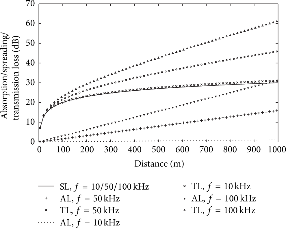
Assuming a target SNR = 20 dB and noise level = 70 dB, the analytical results corresponding to the variation of transmission loss with frequency of operation and distance between the sensor nodes as expressed by (3) are plotted in Figures 4 and 5 for shallow water and deep water environments, respectively. Transmission loss is the sum of spreading loss and absorption loss. Spreading loss is independent of frequency, whereas absorption loss increases with frequency and the distance between nodes. Since spreading is cylindrical ( $k=1$ ) for shallow water environment and circular ( $k=2$ ) for deep water environment, the variation of spreading loss with distance is linear in shallow water, while it is quadratic in deep water.

Figure 4

Variation of propagation losses in shallow water (analytical).

Figure 5

Variation of propagation losses in deep water (analytical).

Assuming tunable transmit power $P_t$ , fixed receive power $P_r=0.075$  W, fixed packet length $L=400$ bits, and bandwidth efficiency of modulation $\alpha =0.5$ [3, 11] in (7), the effect of hop length and channel bandwidth on per-hop energy consumption is plotted in Figures 6 and 7 for shallow water and deep water, respectively. The variation is sharper for deep water since the transmission loss is proportional to the square of the hop length here. From the diagrams, it is evident that, in the energy-constrained underwater environment, direct single hop communication is not feasible over large distances. Also, due to the distance-dependent bandwidth in the underwater scenario, short-range communication is advantageous in two ways, and the effect is more significant in the deep water scenario. Simulation results give slightly higher values than analytical ones due to the presence of distance-independent fixed costs in transmission.

Figure 6

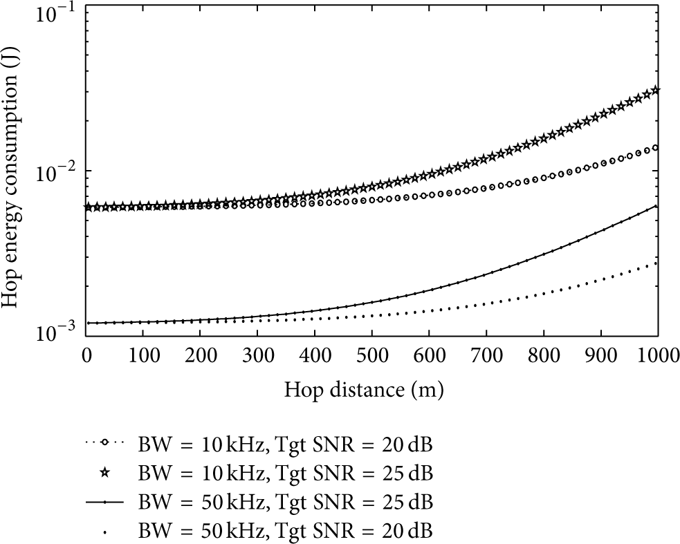
Hop energy consumption in shallow water (analytical).

Figure 7

Hop energy consumption in deep water (analytical).

The analytical and simulation results corresponding to the relaying overhead and network lifetime in a dense/connected network have been obtained and plotted. Assuming 40 sensor nodes uniformly distributed in a circular area of radius 1000 m, with the communication range of the static sensor nodes fixed at a very low value of 50 m (for underwater sensors, less than 1 km is short range and 50 m is considered to be very short), variation of per node energy consumption with proximity to sink as computed using (10) and (11) for ad hoc multihop architecture and MS-based architecture, respectively, is illustrated in Figure 8. As expected, it demonstrates the increased relaying overhead of nodes near the static sink that results in the “hot spot” effect in ad hoc multihop approach contrasted with balanced and reduced energy consumption of nodes in MS-based scheme.

Figure 8

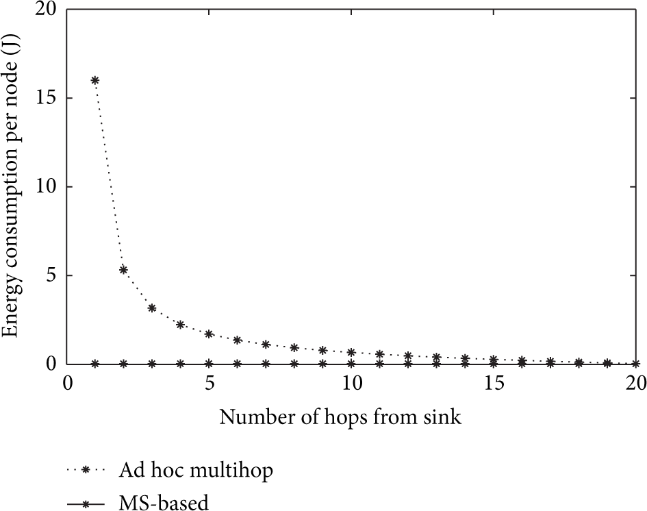
Variation of per node energy consumption with proximity to sink (analytical).

Using the values of hop energy consumption obtained from (7) for different transmission ranges and assuming each static sensor node having an initial energy of 10000 Joules, maximum number of transmissions that can be afforded by a sensor in the MS-based architecture is computed using (15). It is interesting to observe that this value decreases with an increase in transmission range (due to high transmit power requirement), but it is independent of the data generation rate. With each node generating packets of length 50 bytes each and using a channel bandwidth of 10 kHz, the mean lifetime of the network (in days) for different transmission ranges and data reporting rates is illustrated in Figure 9. It is evident that, for a fixed data reporting rate, the lifetime of each node and thus the entire network can be enhanced by adopting short range high bandwidth communication, wherever possible.

Figure 9

Mean network lifetime: MS-based data collection (analytical).

Assuming the radius of the deployment area to be 1000 m, the relative improvement in network lifetime, as indicated by the lifetime improvement factor η in (19), has been evaluated for different transmission ranges, traffic types (CBR and Poisson), packet generation rates, and MS arrival rates and has been illustrated in Figure 10. We have considered the network to be alive till the first node dies due to energy depletion. The results demonstrate the superior performance of MS-based architecture over ad hoc multihop scheme as well as the advantage of using very low transmission range. The relative improvement of the MS-based scheme over multihop network is more pronounced for large and energy-constrained networks. It is interesting to observe that, even though the network lifetime reduces with the data generation rate in both cases, the lifetime improvement factor is independent of traffic type, data generation rate, and MS arrival rate. Another interesting observation is that, if the transmission range and the radius of deployment are same, there exists direct single hop communication between the source and the sink, resulting in no relaying overhead and no rationale in opting for MS-based scheme. However, such situations will never occur in practical UWSN deployments because of the heavy energy cost, high bit error rate, and very limited bandwidth of long range single hop communication in the underwater environment.

Figure 10

Improvement in mean network lifetime due to mobility.

The delay performance of the mobility-assisted scheme is not comparable with that of ad hoc network since the former takes much larger time for data collection. Hence, we have tried to demonstrate the factors affecting this delay and to compare the delay performance of different analytical models for MS-based data collection, as these models represent variants of the generic scheme for MS-based data collection. The network scenario considered for delay analysis with all the three analytical models is the same: a square area of size 2000 m × 2000 m with 10 sensor nodes randomly distributed in the deployment area with each sensor node having sufficient buffer space to avoid buffer overflow. Controlled mobility of the MS along trajectory A is used for simulations and the input load is varied by varying the packet generation rate.

Assuming sufficiently large values of K such that any packet generated in one cycle time of the MS is transferred in the next visit of the MS itself, the delay performance of the Bulk Service Queueing model for different MS mobility patterns as evaluated using (25) has been plotted in Figure 11. For same data generation rate and MS velocity, delay is least for the deterministic motion of the MS and it increases with the variance of the MS arrival distribution. Sensor buffer occupancy also exhibits the same behaviour as depicted in Figure 12. Hence, controlled and deterministic motion of the MS is the most desirable one, wherever deployment permits.

Figure 11

Influence of MS mobility on latency: Bulk Service Queue model (analytical).

Figure 12

Effect of MS mobility on buffer occupancy: Bulk Service Queue model (analytical).

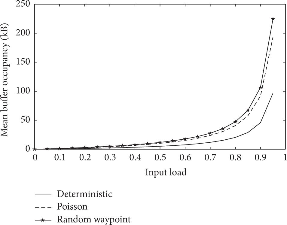
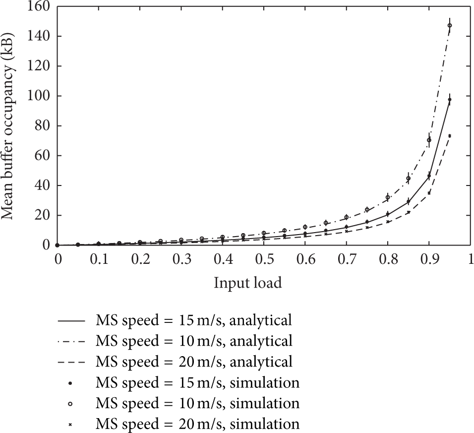
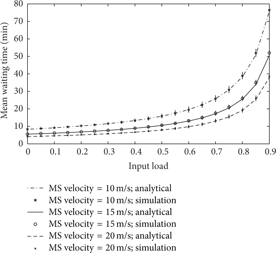
With the same assumptions and using deterministic motion of MS in the Bulk Service Queueing model, the variation of mean queueing delay of packets with varying input load and speed of MS is plotted in Figure 13 and the corresponding buffer occupancy computed using (29) is compared with the simulation results in Figure 14. Since increasing the speed of MS is equivalent to increasing its arrival rate μ at the sensor, both message waiting time and sensor buffer occupancy decrease with increase in MS speed. However, the speed of MS cannot be increased beyond a limit, due to practical reasons. Also, an increase in network load (due to increase in number of nodes and/or data generation rate) leads to increased message delay and buffer occupancy. If the packet arrival rate λ exceeds the net service rate $K\mu$ , system stability is lost and the delay performance parameters increase exponentially. Hence, $\lambda ,K$ , and μ are the design parameters that can be tuned for desired delay performance, and given any two of these three parameters, the third should be properly chosen to ensure stability, minimize delay, and avoid buffer overflow and packet loss.

Figure 13

Variation of mean waiting time: Bulk Service Queue, controlled motion of MS.

Figure 14

Mean buffer occupancy: Bulk Service Queue, controlled motion of MS.

The mean queueing delay obtained using $\text{M}/\text{G}/\mathrm{1}$ queue with vacation for different values of data generation rate and different speeds of the mobile sink have been plotted in Figure 15. Similar to Bulk Service Queueing, the mean waiting time increases with the input load and decreases with the speed of the MS. It is seen that the values obtained by the analytical technique (discussed in Section 4.2.2 and using (32)) closely match with that obtained from simulation. With the same network scenario, same input load, and same MS speed, the values obtained with Bulk Service Queueing model are larger than those with $\text{M}/\text{G}/\mathrm{1}$ vacation model because the former behaves like the gated service scheme of the polling model and the latter like the exhaustive service scheme. In Bulk Service Queue model with large value of K or polling model with gated service, upon visiting a node, MS collects the packets generated and buffered till its arrival instant. In $\text{M}/\text{G}/\mathrm{1}$ with vacation and polling with exhaustive service, MS collects all the packets buffered so far, plus the packets being generated when the already buffered packets are being transferred. As indicated by (35) and (36), polling with exhaustive service results in lower mean waiting time compared to polling with gated service.

Figure 15

Mean waiting time: $\text{M}/\text{G}/\mathrm{1}$ queue with vacation, controlled motion of MS.

Figure 16 shows the average buffer occupancy results obtained with the $\text{M}/\text{G}/\mathrm{1}$ queue with vacation model. Similar to the case of mean queueing delay of packets, the values obtained with this model are larger than those obtained with the Bulk Service Queue model. As expected, the number of packets awaiting their turn for transmission increases with the input load and decreases with the frequency of MS visit. Since insufficient buffer space will lead to buffer overflow and packet loss, this result allows us to design the appropriate sensor buffer size according to the application requirement and the MS arrival pattern. The sensor buffer occupancy is minimum when the MS leaves a sensor and maximum when it approaches the sensor. Thus, the maximum buffer occupancy is the mean cycle time multiplied by the packet generation rate. If the application is delay-tolerant but loss-sensitive, it is not sufficient that the sensor buffer size just exceeds the mean buffer occupancy. For such applications, the sensor buffer space should be chosen to be greater than or equal to the maximum buffer occupancy (at the MS arrival instant).

Figure 16

Mean buffer occupancy: $\text{M}/\text{G}/\mathrm{1}$ queue with vacation, controlled motion of MS.

Assuming controlled motion of the MS with 10 sensor nodes (having infinite buffer size) placed at equal distances, the mean cycle time of the MS, pause time (data upload time) of the MS at a sensor, and average waiting time of a message have been evaluated using (33), (34), (35), and (36) and illustrated in Figure 17. As the input load increases (due to increase in number of nodes, data generation rate, or mean message service time), the mean waiting time also increases. In terms of mean waiting time, exhaustive service is superior to gated, whereas the mean cycle time is same for both policies. At light loads, the mean cycle time of the MS and the mean waiting time of the message are dominated by the MS walk time, while at heavy loads, they are dominated by the service time (pause time) at sensors.

Figure 17

Polling model: waiting time, pause time, switch-over time, and cycle time (analytical).

The mean waiting time for different values of data generation rate and MS speeds using the polling model with exhaustive service and controlled motion of MS is exactly same as that of $\text{M}/\text{G}/\mathrm{1}$ queue with vacation model and hence not repeated. The variation of the mean buffer occupancy with varying load and MS speeds also shows exactly same behaviour as that of $\text{M}/\text{G}/\mathrm{1}$ with vacation.

Assuming sufficiently large buffer size to avoid buffer overflow, no losses in communication, and controlled motion of the MS with a speed of 15 m/s, the impact of data generation rate and service batch size K (maximum number of packets collected from each sensor in a single visit) on Packet Delivery Ratio (PDR) is studied using the Bulk Service Queue model and illustrated in Figure 18. Under stable condition, all the packets generated in one cycle time of the MS are transferred in the next visit of MS, and thus PDR is 1. At low data generation rates, low batch size is sufficient for good delivery performance, whereas at high data generation rates, high batch size is necessary for system stability and successful data delivery. As the data generation rate exceeds the net service rate ( $K\mu$ ), stability condition is lost and PDR starts dropping, finally reaching zero.

Figure 18

Impact of data generation rate and service batch size on PDR: Bulk Service Queue (analysis).

With the controlled motion of the MS at 15 m/s, simulation results illustrating the combined effect of sensor buffer size and data generation rate on PDR are shown in Figure 19. Assuming no loss in transmission, packet loss (if any) occurs due to buffer overflow and hence the delivery ratio is strongly dependant on the buffer size. For a fixed packet arrival rate, as the buffer size is increased, delivery ratio increases (sharply for low arrival rates and slowly for high arrival rates) and once it reaches a maximum value, it remains insensitive to buffer size. For the same target delivery ratio, small buffer size is sufficient under low packet arrival rates, but as the arrival rate is increased, buffer space requirement also increases. Also, for the same buffer space available, as the data generation rate increases, delivery ratio decreases. Hence, this graph provides us an insight into how to decide the sensor buffer size for a particular application.

Figure 19

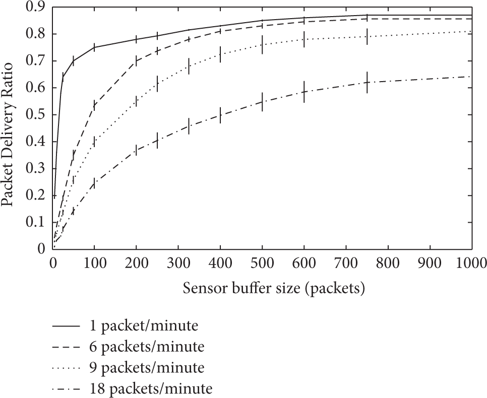
Effect of finite buffer size and data generation rate on PDR (simulation).

Fixing the width of the routing pipe B to be 100 m in multihop communication using VBF, variation of PDR with node density in ad hoc multihop and MS-based data collection schemes is shown in Figure 20. Assuming infinite buffer size and no communication errors, ideally the delivery ratio should be 1 for MS-based data collection scheme, but when we run the simulation for a finite amount of time, all the sensor nodes may not be detected and hence the delivery ratio is slightly less than 1. In multihop ad hoc network using VBF, delivery ratio is very small for low node density, due to connectivity gaps in the network. As the node density is increased, PDR increases due to improved connectivity, reaches a maximum value, and then remains almost constant. Also, for a fixed node density, increasing the communication range of sensor nodes or the width of routing pipe results in enhanced PDR; however, it is not recommended due to increased power consumption. Since MS-based data collection fills connectivity gaps, PDR is independent of node density. Also, transmission range of 250 m has given good results in MS-based scheme and hence there is no meaning in increasing it further. The results show that MS-based scheme is the better option for sparse and energy-constrained networks, to achieve successful packet delivery.

Figure 20

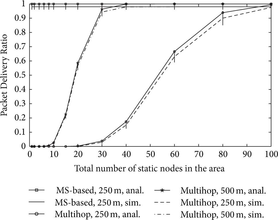
Packet Delivery Ratio with multihop and MS-based data collection.

Network throughput is the number of bits transferred per unit time. Simulation results showing the impact of buffer size and data generation rate on network throughput under the assumption of controlled motion of MS at 15 m/s are given in Figure 21. As expected, for fixed buffer size, throughput increases with the data generation rate. For a fixed data generation rate, it increases with the buffer size initially and then remains constant at the maximum possible value.

Figure 21

Effect of finite buffer size and data generation rate on throughput (simulation).

For investigating the influence of MS trajectory on the performance metrics of our data collection scheme, we have fixed the input load ρ at 0.4 and tuned the transmission range of the sensors to be large enough to be detected by the MS during its travel. Assuming controlled deterministic motion of the MS along three typical trajectories shown in Figure 3, the variation of mean cycle time of MS, mean waiting time of messages, energy consumption per packet received, and the PDR have been determined and illustrated in Figures 22 and 23 and Table 1. For a fixed speed of 15 m/s and exhaustive service policy, the mean cycle time and the mean waiting time are evaluated using (33) and (35), respectively, and illustrated in Figures 22 and 23. It is observed that, among the trajectories considered for comparison study, cycle time of MS and waiting time of messages are smallest for trajectory C and largest for A. The impact of trajectory on delay is more pronounced at light loads than at heavy loads. This is because the cycle time and waiting time are dominated by the MS travel time at light loads, and by the data upload time at the sensors at heavy loads.

Table 1

Impact of MS trajectory on energy efficiency and PDR (application 1: delay-tolerant; application 2: delay-sensitive with delivery deadline 3 minutes).

MS trajectory	Commn. range	Energy consumption	PDR (%)
(as in Figure 3)	(metres)	(mJ/packet)	Application 1	Application 2
A	250	3.17	99.8	32.7
B	500	5.325	99.8	57.2
C	750	7.825	99.8	71.3
Static sink	1000	10.7	99.8	99.8

Figure 22

Mean cycle time variation with trajectory (analytical).

Figure 23

Variation of mean waiting time with MS trajectory and speed (input load $\rho =0.4$ ).

At the same time, though the MS requires more time to complete one cycle by following trajectory A, it ensures improved delivery performance in a highly constrained environment. This is because of the reduced transmit power requirement of static sensors to ensure short-range, high data rate single hop connectivity with the MS. Due to the requirement of increased transmission range of static sensors while using trajectory C, their energy consumption will be the highest with trajectory C and the lowest with trajectory A. Since we have fixed the transmission range to be sufficiently high such that all the nodes in the deployment area will be covered by the MS by travelling along the trajectory, PDR with all the three trajectories, as observed in simulation, nearly equals the theoretical value of 1 for a delay-tolerant application. However, for applications with tight deadline requirements, packets missing the deadline are discarded. Since the trajectory C offers the best delay performance, in the case of delay-sensitive applications, its delivery performance (as indicated by PDR) is also the best. Thus, the results illustrate a trade-off between energy consumption and latency and acts as a guide to select the MS trajectory according to the application requirements; that is, trajectory A with transmission range 250 m is suitable for a delay-tolerant application in highly constrained environment, whereas, trajectory C with 750 m range will be more suited for a delay-sensitive application in a network with nodes having higher energy reserves. The static sink with direct single hop communication supports time-critical applications, at the cost of very high energy consumption. For transmission range and transmitting power level fixed at small values, MS following trajectory A achieves better coverage and successful data delivery than B, C, and static sink, though at the cost of increased delay.

6. Discussion

Exploiting controlled mobility of sensor nodes for improving data collection performance of resource-constrained and disruption-prone underwater sensor networks has been presented and the analytical techniques to estimate data collection latency and sensor buffer requirement prior to network deployment have been discussed. The proposed framework is found to be effective for delay-tolerant sensing applications and in situations where network lifetime is more important than message latency. Now let us see what exactly is the advantage of analysing the system with three different delay models and how effectively the results can be used for future research in this area.

6.1. Comparison of Delay Models

The different analytical models of latency computation—Bulk Service Queue, $\text{M}/\text{G}/\mathrm{1}$ queue with vacation, polling with exhaustive service, and polling with gated service—represent different service models of the proposed MS-assisted data collection framework. Having presented the results of the latency analysis using these models, a comparative study of the results obtained reveals some interesting information that we hope will be useful for the network designer.

Assuming controlled motion of the MS (with speed fixed at 15 m/s) in a square area of size 2000 m × 2000 m, and 10 sensor nodes uniformly distributed in this area, generating packets of size 50 bytes, Table 2 gives a comparison of the mean waiting time as evaluated using the different delay models. This comparison of the latency performance of different analytical models that we have performed is, in fact, comparison of the different service models of the proposed MS-assisted data collection framework. For a fixed input load, polling model with exhaustive service policy and $\text{M}/\text{G}/\mathrm{1}$ queue with vacation model provide optimum waiting time and buffer occupancy. An interesting observation is that the behaviour of $\text{M}/\text{G}/\mathrm{1}$ queue model with vacation is exactly the same as the exhaustive service scheme of the polling model and thus both models turn out to be one and the same.

Table 2

Mean message delay with different models.

Mean arrival rate	Analytic model used	Mean waiting time
(Packets/minute)		(Minutes)
10	Polling: exhaustive service	6.92
10	Polling: gated service	7.1
10	Bulk Service Queue	6.99
10	M/G/1 with vacation	6.91
60	Polling: exhaustive service	12.5
60	Polling: gated service	13.2
60	Bulk Service Queue	13.1
60	M/G/1 with vacation	12.52
100	Polling: exhaustive service	52
100	Polling: gated service	55.2
100	Bulk Service Queue	55.1
100	M/G/1 with vacation	52.05

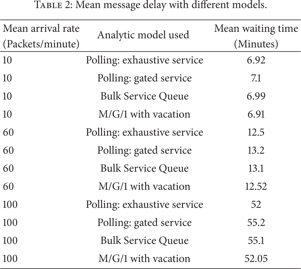
It is observed that the Bulk Service Queueing model with $K\ge \mathrm{1}$ is similar to the K-limited polling model, but the former permits easy analysis with a finite buffer space, which is not so with the latter one. Also, with sufficiently high values of service batch size K and sensor buffer space SB, the Bulk Service Queueing model behaves like the gated service polling model. The mean waiting times and sensor buffer space requirements with these models are larger than those of the polling with exhaustive service and $\text{M}/\text{G}/\mathrm{1}$ queue with vacation models. However, they exhibit a desirable characteristic which is significant especially in asymmetrical systems, that is, systems in which the packet generation rates (and thus the offered load) vary heavily among the sensors. All sensors receive fair treatment under these policies since the packets buffered till the polling instant alone are collected in the current visit of the MS, in contrast to the other two service models where the nodes with high data generation rates may prevent the MS from visiting the lightly loaded queues.

Out of the three analytical models for delay performance, the polling model is the most versatile and flexible one, mainly because of its capability to incorporate different service policies, scheduling disciplines, and optimization schemes. The polling model, with its number of variants, can accurately model the average case and worst case latency performance of mobility-assisted data collection framework.

6.2. Scope for Further Study

As a future work, we plan to extend the proposed framework to 3-dimensional network with multiple mobile sinks and to formulate a cross-layer adaptive approach for improved data collection performance. It is also planned to investigate techniques for reducing data collection latency and optimizing the network performance dynamically according to application requirements and network conditions. Machine learning techniques need to be explored in the underwater DTN schemes to improve their adaptability to the changing environment. Optimization algorithms can be developed to design better MS trajectories for periodic as well as event-driven data collection. Another interesting work will be the investigation of the impact of traffic models and MAC on network performance.

7. Conclusion

In this paper, we have considered application-oriented and energy-efficient data collection schemes for sparse underwater acoustic sensor networks, considering them as delay-tolerant networks. Exploiting the controlled mobility of underwater sink node, we have achieved high data delivery ratio and enhanced network lifetime, at the cost of increased message latency. The MS-based scheme has been found to be the only feasible option in disconnected networks and the more energy-efficient option in all networks. Realistic models for energy consumption, network lifetime, Packet Delivery Ratio, and message latency have been presented to analyze the proposed framework. The analytical models presented permit the evaluation of the network performance metrics prior to actual deployment of nodes.

Delay analysis was done based on three different queueing models, a comparison of which reveals that each model is suitable for some specific application requirements. The Bulk Service Queueing model is suitable for modelling a system in which the MS follows a round-robin approach of visiting the sensors and collects a fixed number of packets from each sensor. It also facilitates modelling of finite buffer systems, which is more realistic, but the analysis of which is not easy with the other models. The $\text{M}/\text{G}/\mathrm{1}$ queue with vacation can effectively model a system in which, upon visiting a sensor, the MS collects all the packets buffered so far plus the packets being generated when the already buffered packets are being transferred. Polling model is found to be the most versatile and flexible one among the three models considered, with its k-limited service scheme supporting periodic data collection with fair treatment given to all sensors, exhaustive service scheme being the optimal one in terms of mean waiting time and buffer occupancy, and the gated service scheme standing in between the other two in terms of delay and fairness metrics. Both analytical and simulation results show that the Bulk Service Queueing model with sufficiently large service size and buffer space behaves like the gated service scheme of the polling model.

We have developed the simulation platform (in C++ and OTCL) by incorporating the DTN routing features and the queueing models into the NS-2 based network simulator, Aqua-Sim. Thus, an enhanced simulation environment is made available for further research and predeployment investigations in this novel area. Simulation results closely match with the analytical ones and the proposed scheme is suitable for nontime-critical applications.

This paper has focused on the performance metrics of Packet Delivery Ratio and energy consumption, without giving much importance to the timely delivery of data. Hence, the scheme is suitable only for delay-tolerant applications. With very short distance between static sensor and MS, optical communication with very high data rate is feasible, thus minimizing the service time at the sensors, thereby minimizing the data collection latency to a great extent, especially at heavy load conditions. For delay-sensitive applications, the emergency data or request for service will have to be routed to the sink directly or through ad hoc network. The inevitable trade-off between energy consumption and latency has to be considered according to the application requirement and network connectivity.