D3D-MDS: A Distributed 3D Localization Scheme for an Irregular Wireless Sensor Network Using Multidimensional Scaling

Abstract

This paper proposes a distributed localization algorithm which can be applied to an irregular three-dimensional wireless sensor network, considering the algorithm accuracy and complexity. The algorithm uses clusters to eliminate the multihop distance errors. An anchor node position optimization scheme is proposed to maximize the uniformity of each subnetwork. The proposed algorithm also employs a new three-dimensional coordinate transformation algorithm, which helps to reduce the errors introduced by coordinate integration between clusters and improves the localization precision. The simulation and performance analysis results show that the localization accuracy of the D3D-MDS algorithm increases by 49.1% compared with 3D-DV-HOP and 38.6% compared with 3D-MDS-MAP. This distributed localization scheme also demonstrates a low computational complexity compared with other centralized localization algorithms.

1. Introduction

Localization has been an important topic in data-centric wireless sensor networks (WSNs) due to the special association between location information and the relevance of sensory data. Recently, a gradual but marked shift in the focus of 3D localization has taken place. While the 3D technique brings WSNs closer to reality, the localization complexity in computation and accuracy can be much higher than a 2D case.

The most straightforward method for 3D localization is to use the global positioning system (GPS). Nevertheless, having each node GPS-equipped is extremely expensive for large scale wireless sensor networks. Recently there has been growing interest in 2D localization protocols that use the connectivity information only [1]. This aims to produce a relative coordinate system for a network without reliance on extra hardware supplements [2–4]. These schemes can accurately recover the original network topology, up to scaling and rotation. Among the many studies, multidimensional scaling (MDS) based localization techniques have been proved to compute locations of high accuracy and request low node density. A state-of-the-art MDS based algorithm, MDS-MAP [5], takes an internode hop distance/estimated distance matrix as input and generates a set of relative coordinates for each node.

Currently, 3D localization has been widely investigated in the area of underwater sensor networks. Many centralized localization schemes are proposed to estimate node locations, such as 3D-DV-HOP [6] and 3D-MDS [7]. However, these schemes either suffer from high computation complexity or heavily depend on assumptions about the network environments, such as dense anchor deployment, the availability of depth information, and a relatively small network size. None of these schemes can work with connectivity information alone (or with a constant number of anchors) in an irregular large scale 3D WSN.

The above observation motivates our work in developing an effective 3D localization approach which can be used in a large scale wireless sensor network regardless of topology. Most importantly, a distributed localization algorithm is highly preferred in large scale 3D WSNs as it can achieve network localization at respective low computational cost. For some cases, a distributed localization algorithm could even fulfill partial localization.

In this paper, we propose a distributed 3D localization scheme for an irregular wireless sensor network using multidimensional scaling (D3D-MDS). The algorithm uses clusters to eliminate the multihop distance errors. An anchor node position optimization scheme is proposed to uniform each subnetwork. Also a new three-dimensional coordinate transformation algorithm inspired by camera calibration principle of computer vision is introduced in the proposed algorithm to reduce the errors of coordinate integration between clusters and improve the localization precision. The empirical result demonstrates the capability of D3D-MDS in higher accuracy and low computational cost. The contribution of proposed algorithm lies in the high localization accuracy, relative low computational complexity, and the distributed fashion of localization.

The remainder of this paper is organized as follows. Section 2 outlines the previous algorithms carried out on 3D localization and valuable ideas in 2D plane with respect to localization. The D3D-MDS algorithm is then described in detail in Section 3. Section 4 presents a description of the simulation scenarios and results. Algorithm performance evaluation in terms of accuracy and complexity is also discussed in this part. Finally, in Section 5, the conclusion and future work are listed.

2. Related Works

While extensive studies focus on localization techniques in two-dimensional space, few approaches have been proposed for three-dimensional locationing. Landscape 3D [8] is proposed as one of the first proposed robust localization techniques for 3D sensor deployments using range-based approach. Landscape 3D introduces the concept of mobile location assistants (LA) that are aware of their moving positions through GPS. Each location-unaware node uses RSSI to estimate its own location through LAs that are around. USP [9] tackles the localization problem in sparse 3D underwater sensor networks where the depth information of deployed sensors is available. USP utilizes a projection technique to map the problem to make using range estimation techniques for 2D terrestrial sensor networks possible. Shi et al. [10] introduce a 3D localization approach for WSNs. Similar to Landscape-3D, their localization approach makes use of a mobile beacon, which emits ultra-wideband (UWB) signals to achieve location positioning. Upon reception of the UWB signals, each sensor node measures the distance to the mobile anchor using the TOA technique. Although these methods are independent of node densities and network topologies, the major drawback relied on mobile beacon or extra hardware for the network.

Another kind of major methods on 3D localization employs centralized algorithm to compute the actual coordinate of each unknown node instead of using range-based approaches. The centroid-based approach [11] is among the earliest works of connectivity-based localization. A node estimates its location simply by calculating the centroid of audible anchors’ locations. If anchors are placed uniformly, then the localization can be achieved with high accuracy. However, the accuracy cannot be assured for ad hoc or mobile WSNs with such technique. Other centralized algorithms, like DV-HOP, MDS-MAP, and so forth, are modified from 2D-plan scenarios. In [12] the authors propose cluster-based approach named CBLALS. In each cluster, the intercluster range measurement errors are corrected using triangle principle. The evaluation of CBLALS with respect to DV-Distance (3D) shows that CBLALS has much better positioning accuracy than DV-Distance (3D). A novel centroid localization method that significantly improves the basic centroid localization algorithm is presented in [13]. Each unknown node randomly selects four anchor nodes to form a series of tetrahedrons which are used to calculate its own position. However, for a large scale wireless sensor network, with the limited power and computation capability of each sensor node, centralized algorithms can be extremely expensive at cost of computational and time complexity.

CATL [14] is a recent state-of-the-art localization algorithm that can be adopted into a 3D scenario. The key idea of CATL is to identify notch nodes where the hop-count of the shortest path between the nodes deviates the true Euclidean distance. CATL then uses an iterative notch-avoiding multilateration scheme to localize the network. The performance of CATL heavily depends on proper deployment of some beacon nodes. In addition, due to the iterative procedure, CATL suffers from error propagation.

Zhao et al. [15] propose a localization algorithm for complex 3D surface. It formulates the localization problem under a practical setting with estimated link distances (between nearby nodes) and nodal height measurements and introduces a layered approach to promote the localizability of such 3D surface sensor networks. The nodal height measurements can be obtained by measuring atmospheric pressure through pressure sensors. The algorithm employs the idea that 3D surface localization problem can be reduced to the localization problem on 2D plane with the known nodal height. However, the extra hardware is quite expensive; for example, the Crossbow MTS400/MTS420 sensor board equipped with intersema MS55ER pressure sensor is priced at 467 US dollars. In addition, the layered approach in this algorithm is extremely computationally expensive. It is not suitable for large scale energy-constrained WSNs.

3. A Distributed 3D Localization Scheme for an Irregular Wireless Sensor Network Using Multidimensional Scaling

In our paper, we propose a distributed localization technique in 3D wireless sensor network environments where sensor nodes can be randomly deployed regardless topology. For complete network localization, we assume that the network is fully connected, which means at least one routing path exists between any pair of sensor nodes on the network. Also, no sensor node has mobility in the network. The rough procedures of 4 steps are shown as Algorithms 1, 2, 3, and 4 and the details of each step will be introduced next.

• (I)

Anchor node placement: assuming we have the boundaries of the network (boundary identification is out of the scope of this work as it was fully discussed in work [16–19]), we identify a series of edge nodes from the network boundaries. Then an anchor node configuration algorithm is proposed in this part to achieve relatively high localization accuracy by optimizing the anchor nodes placement.

(II)

Node clustering: the subnetworks are generated from node clustering. Each subnetwork is identified by an anchor node and a group of unknown nodes nearby. After node clustering, each subnetwork will achieve relative localization by MDS algorithm. The node clustering algorithm will guarantee each cluster is composed of unknown nodes which have the minimum hop information to their cluster head (anchor node).

(III)

Local relative map establishment: we propose an improved MDS technique to build the relative map for each cluster. MDS-MAP has a computational overhead of $O(n^3)$ in a network of n nodes and, in particular, results in significant localization accuracy error in environments with holes. Thus, this paper proposes an improved MDS algorithm which yields smaller accuracy error in all environments.

(IV)

Global map establishment: finally, we will combine the coordinates of all the clusters into a global map. Note that the combination process will need to be known each sensor in the cluster of the new coordinates. We develop a new three-dimensional coordinate transformation algorithm inspired by camera calibration principle of computer vision to reduce the errors of coordinate integration between clusters.

Algorithm 1: Anchor nodes configuration.

 begin

   input: A bitmap $Im$ of size $w\times l$

   output: A partition of the bitmap

(1)  for each sensor node   do

(2)    establish the neighbor table by receiving the messages from other nodes;

(3)    Arbitrary node p whose order number is p obtains its k-hop

      neighborhood $N_p(k=\mathrm{1,2})$ , then $n{\hspace{0.17em}\hspace{0.17em}N}_p$ will be obtained.

(4)    Here we let $d_p$ denotes the the network connectivity of p within two hops

(5)    $\bar{d}$ is the average network connectivity, which is calculated from 2/5 of $n\hspace{0.17em}\hspace{0.17em}{N}_p$ .

   if   $d_p<(\mathrm{1}-\mathrm{\omega })\times \bar{d}$ ( $\mathrm{0}<\mathrm{\omega }<\mathrm{1}$ )  then

(6)   nodes p is an edge node.

(7)     for  each edge node p  do

(8)   if  no nodes is marked as an anchor node in this neighborhood   then

(9)     flooding a message within $EdgeSpacing$ ; an anchor node position is identified

(10)    if  the flooding message is heard   then

(11)    cancel the flooding

Algorithm 2: Node clustering.

 Data: anchors nodes, unknown nodes

 Result: Based on the anchor nodes clusters

(1) begin

(2)    m represents the number of anchors nodes in the network;

(3)    for   $i\leftarrow \mathrm{1}$   to  m  do

(4)    for   $j\leftarrow \mathrm{1}$   to  m  do

(5)     if  i  and j  can communicate with each other directly   then

(6)      if   $i\ne j$   then

(7)        $neighbor\_matrix(i,j)=\mathrm{1}$ ;

(8)      else

(9)        $neighbor\_matrix(i,j)=\mathrm{0}$ ;

(10)     else

(11)       $neighbor\_matrix(i,j)=Inf$ ;

(12)   $neighbor\_matrix$ can indicates the connectivity relationship between nodes;

    $ShortestPath\hspace{0.17em}\hspace{0.17em}(neighbor\_matrix)$ ;

(13)  n represents the number of unknown nodes in the network;

(14)  for   $i\leftarrow \mathrm{1}$    $to$   n  do

(15)   if  it has a minimum hop with an anchor node or one more anchor node  

     then

(16)    put it into the cluster of the anchor node;

(17)  Then clusters are built and some special nodes called common nodes may exist more than one cluster.

Algorithm 3: Local relative map establishment.

 Data: clusters based on the anchors nodes

 Result: the relative maps in each cluster

(1) begin

(2)  for  each cluster   do

(3)   Corporator of each cluster obtain the hop-count square matrix $D_i$ ;

(4)   Compute the inner product matrix $B_i$ ;

(5)   Apply singular value decomposition on matrix $B_i$ ;

(6)   Extract the first three largest eigenvalues and eigenvectors;

(7)   Obtain the relative map of this cluster.

Algorithm 4: Global map establishment.

 Data: the local relative coordinates of k clusters

 Result: the global map of the netwok

(1) begin

(2)  for   $i\leftarrow \mathrm{1}$   to   k  do

(3)   for   $j\leftarrow \mathrm{1}$   to   k  do

(4)    work out the common nodes number matrix between cluster i and cluster j;

(5)    find out the coordinates of the common nodes between clusters;

(6)    screen out the coordinates of other ordinary nodes in each cluster;

(7)  sort the clusters by the number of the common nodes;

(8)  for   $m\leftarrow \mathrm{1}$   to $(k-\mathrm{1})$   do

(9)    each time screen two clusters sharing most common nodes to merge;

(10)   firstly, use the coordinates of common nodes in two clusters to work out the

    parameters of 3D transformation algorithm;

(11)   secondly, normalize the other ordinary nodes’ coordinates in each clusters until there is only one big cluster.

(12)   finally, the global map contain all the relative coordinates of the network.

3.1. Anchor Nodes Placement

Anchor node placement plays an important role in the quality of spatial localization. As we all know, nodes near the network periphery are more representative of the network layout than interior nodes. In our work, we assumed that network boundary is available and used the edge nodes [20] to find the optimized positions for anchor nodes. Although edge nodes share the common property of being close to the network periphery, they may not cover all the network boundaries. The edge nodes are those representative nodes used to obtain all the major corners in the network. Therefore, the edges nodes detection is more effective than detecting a full and tight boundary. Based on the network edge detecting method [20], we propose an anchor node configuration optimization algorithm to achieve relatively high localization accuracy.

3.1.1. Finding the Network Edge Nodes

The network edges represent a set of boundary nodes where, near the periphery of the network, the identification of edge nodes is described as follows.

• (1)

Each node obtains its own neighbor nodes to establish a neighbor table. Then all nodes exchange information with its own neighbor node to obtain its two hops neighbor nodes. The reason we choose the network connectivity within two hops is that the influence of the network connectivity within one hop is so susceptible to communication noise that large error can be made.

(2)

All nodes in the network broadcast message packets in the form of flooding. The message packet contains the ID number of the node and network connectivity within two hops, so that each node can obtain the network connectivity within two hops of the other nodes. Through the above data, we can obtain a roughly uniform random sample about the network connectivity within two hops of all nodes. In order to avoid the small deviation of border nodes network connectivity and simplify the operation, the average network connectivity $\bar{d}$ within two hops is calculated from a fraction of samples (we use 2/5 in our experiments).

(3)

Based on the network connectivity $\bar{d}$ within two hops, the network edge nodes can be screened in accordance with the following methods: arbitrary sensor node p compares its own network connectivity $d_p$ within two hops and with the average network connectivity $\bar{d}$ within two hops, if $d_p<(\mathrm{1}-\omega )\times \bar{d}$ , ω satisfied $\mathrm{0}<\omega <\mathrm{1}$ , and then the node p will be marked as the edge node. Through this method, we can get a set of the edge nodes of the network.

3.1.2. Anchor Nodes Placement

Having obtained the set of the edge nodes of the network, we can deploy anchors nodes on the network edges so that more effective localization can be obtained. The algorithm chooses uniformly sampled distribution of nodes from the set of the edge nodes with density controlled by a small system parameter EdgeSpacing (typically 3 in our setting). Every edge node asynchronously floods a message in its 3-hop neighborhood, it marks itself as one possible anchor position and then notifies the neighborhood. If a node hears such a flood before its own action, then it cancels its own flooding. After a sufficient time, the hop distance of all these selected nodes between each other is roughly the same. The anchors nodes are then placed in the sampled network edges.

3.2. Node Clustering

The purpose of clustering [21] is to subsection the network and reduce the computation of the algorithm and guarantee the accuracy. Each anchor node is selected as a cluster head. There are two conditions that must be considered:

• (i)

all the unknown nodes must be assigned to clusters,

(ii)

each two neighboring clusters must have four common nodes, in order to merge coordinates between clusters.

Based on those two requirements, the node clustering algorithm is described as follows.

• (1)

After all the nodes initialize, every anchor node in the network floods broadcasting packets to neighboring nodes. The packets contain the anchors ID and hop count (initial value is 0).

(2)

Each unknown node maintains a storage list which records the information of minimum-hop anchor node. The basic principle of maintenance is when a node receives a new anchor packet, there will appear two different cases. If the current storage list is empty, the unknown node will store the information of the packet; if not empty, the node will compare the current hop count in the stored packet with the hop count in new anchors packet and the storage list will store the smaller hop count of these two data.

(3)

When each node finishes the above steps, the hop count of the nodes will be plus 1 and it will be transmitted to the node's neighboring node. As a result, every unknown node receives all the anchor packets and updates the storage list. If a node has received the same anchor node information, the storage list will maintain the minimum hop information. It will ensure that the unknown node gets the minimum hop information from anchors nodes.

(4)

After all nodes obtain the smallest hop count information from the corresponding anchor, the unknown nodes will select the anchor node. From the anchor nodes that will be selected the unknown nodes have the smallest hop count, and they put these anchors nodes as its cluster head node [21] and then join the cluster. On the border between two clusters, a node will be a common node if it joined at least two clusters at the same time. In 3D space, merging two coordinate system together must have at least 4 common nodes, which will be introduced in the following part.

3.3. Local Relative Map Establishment

So far the network has been decomposed into several clusters. Every cluster has an anchor node as the cluster head, whose role is in charge of the process of local relative map establishment. Within each cluster, the cluster head computes the shortest distance between each node in current cluster by receiving the information from other nodes in this cluster. Based on the established distance matrix, a local relative map will be established by MDS-MAP algorithm. In this paper, the algorithm based on MDS we uses consists of 4 steps.

Firstly, let $N_i$ be the number of sensors in the network and computes an $N_i\times N_i$ distance square matrix $D_i$ , which represents the square of the pairwise distance between two nodes. Secondly, calculate the inner product matrix $B_i$ of the pairwise distance matrix $D_i$ . The relationship between $B_i$ and $D_i$ satisfied the following formulas: $B_i=-(\mathrm{1}/\mathrm{2})E{D}_{i}E$ , and E represents Nth identity matrix. Thirdly, MDS applies SVD (singular value decomposition) on matrix $B_i$ to extract all eigenvalues and their corresponding eigenvectors of matrix $B_i$ . Finally, the first three largest eigenvalues and eigenvectors give a relative map with relative location for each node.

3.4. Global Map Establishment

After each cluster establishes its local relative map, now we need to combine them to a global map. There are two points that must be concerned: the order of merging cluster and the method for 3D coordinate translation when the global map was established.

• (i)

During the clustering, every two adjacent clusters have some common nodes, whose coordinates are assigned from two different coordinate systems. The merging process of two clusters is started from the greatest weight of a pair of two clusters. Here the weight means the number of common nodes between pairs.

(ii)

3D coordinate merging algorithm is a key step, and the correspondence between two coordinate systems heavily affects the performance of D3D-MDS. We use an improved transformation algorithm to achieve rigid transformation between coordinate systems (each local map has its own coordinate system) so that the relative coordinates of each local map can then be transformed to the absolute global coordinates of the whole network.

3.4.1. 3D Coordinate Transformation Algorithm

The 3D coordinate transformation algorithm is the key of transforming local relative coordinates to global absolute coordinates. There are many algorithms proposed for coordinate transformation in computer graphics, such as Horn algorithms [22] and several other methods [23–25]. The Horn algorithm consists of three main aspects: rotation, transformation and scaling factors. However, in our problem space, relative coordinate systems share the global metrics (the distance/hop counts between each node); therefore, only rotation and transformation are involved when two coordinate systems merge [26, 27].

We propose an approach which uses the homogeneous coordinates to achieve different coordinate merges. Homogeneous coordinates are a coordinate representation method which uses $N+1$ coordinates to describe N coordinates. If the homogeneous coordinates of a point are multiplied by a nonzero scalar, then the resulting coordinates represent the same point. The idea is derived from the camera calibration principle of computer vision as shown in Figure 1. The coordinates of P are in the camera coordinate system $(x_p,y_p,z_p)$ , while in the world coordinates coordinate system is $(X_p,Y_p,Z_p)$ . The transformation formula between these two coordinate systems is shown in

$$\begin{array}{cc}& \left[\begin{array}{c}{x}_p\\ y_p\\ z_p\\ \mathrm{1}\end{array}\right]=\left[\begin{array}{cc}{R}_{\mathrm{3}}{\times }_{\mathrm{3}}& T_{\mathrm{3}}{\times }_{\mathrm{1}}\\ O_{\mathrm{3}}{\times }_{\mathrm{1}}& \mathrm{1}\end{array}\right]\left[\begin{array}{c}{X}_p\\ Y_p\\ Z_p\\ \mathrm{1}\end{array}\right].\end{array}$$

(1)

Figure 1

Coordinate system.

The rigid transformation from world coordinates to camera coordinates needs two kinds of transformation: rotation and translation transformation. As shown in formula (2), $R_{\mathrm{3}}{\times }_{\mathrm{3}}$ represents the rotation transformations which include the rotation transformation of x, y, and z axis. ${\theta }_x$ , ${\theta }_y$ , and ${\theta }_z$ are used to represent the rotation angle of the camera coordinate system around X axis, Y axis, and Z axis of the world coordinate system, respectively. $R_x$ , $R_y$ , and $R_z$ represent the corresponding rotation matrix, respectively:

$$\begin{array}{l}\hspace{1em}\hspace{0.17em}\hspace{1em}{R}_{\mathrm{3}}{\times }_{\mathrm{3}}=R_z{R}_y{R}_x,\\ R_x=\left[\begin{array}{lll}\mathrm{1}& \mathrm{0}& \mathrm{0}\\ \mathrm{0}& \cos {\theta }_x& -\sin {\theta }_x\\ \mathrm{0}& \sin {\theta }_x& \cos {\theta }_x\end{array}\right],\\ R_y=\left[\begin{array}{lll}\cos {\theta }_y& \mathrm{0}& \sin {\theta }_y\\ \mathrm{0}& \mathrm{1}& \mathrm{0}\\ -\sin {\theta }_y& \mathrm{0}& \cos {\theta }_y\end{array}\right],\\ R_z=\left[\begin{array}{lll}\cos {\theta }_z& -\sin {\theta }_z& \mathrm{0}\\ \sin {\theta }_z& \cos {\theta }_z& \mathrm{0}\\ \mathrm{0}& \mathrm{0}& \mathrm{1}\end{array}\right].\end{array}$$

(2)

And $T_{\mathrm{3}}{\times }_{\mathrm{1}}$ in formula (1) represents the translation transformation matrix of original point from world coordinates to camera coordinates.

The proposed approach for coordinate transformation in this paper is described as follows: suppose there are two clusters named cluster A and cluster B, and the 3D coordinates of one point p in both cluster are $(x_A,y_A,z_A)$ in cluster A and $(x_B,y_B,z_B)$ in clustr B. We use formula (3) to merge the two coordinates:

$$\begin{array}{cc}& \left[\begin{array}{c}{x}_A\\ y_A\\ z_A\\ \mathrm{1}\end{array}\right]=M_{BA}\left[\begin{array}{c}{x}_B\\ y_B\\ z_B\\ \mathrm{1}\end{array}\right]=\left[\begin{array}{cc}R& T\\ O& \mathrm{1}\end{array}\right]\left[\begin{array}{c}{x}_B\\ y_B\\ z_B\\ \mathrm{1}\end{array}\right].\end{array}$$

(3)

More specifically,

$$\begin{array}{cc}& \left[\begin{array}{c}{x}_A\\ y_A\\ z_A\\ \mathrm{1}\end{array}\right]=\left[\begin{array}{cccc}{R}_{\mathrm{1}}& R_{\mathrm{2}}& R_{\mathrm{3}}& T_x\\ R_{\mathrm{4}}& R_{\mathrm{5}}& R_{\mathrm{6}}& T_y\\ R_{\mathrm{7}}& R_{\mathrm{8}}& R_{\mathrm{9}}& T_z\\ \mathrm{0}& \mathrm{0}& \mathrm{0}& \mathrm{1}\end{array}\right]\left[\begin{array}{c}{x}_B\\ y_B\\ z_B\\ \mathrm{1}\end{array}\right].\end{array}$$

(4)

$M_{BA}$ is the coordinate transformation matrix from cluster B to cluster A. There are 12 variables, which expressed the rotation matrix R and translational matrix $T=[T_x,T_y,T_z{]}^T$ . The rotation matrix

$$\begin{array}{cc}& R=\left[\begin{array}{ccc}{R}_{\mathrm{1}}& R_{\mathrm{2}}& R_{\mathrm{3}}\\ R_{\mathrm{4}}& R_{\mathrm{5}}& R_{\mathrm{6}}\\ R_{\mathrm{7}}& R_{\mathrm{8}}& R_{\mathrm{9}}\end{array}\right]\end{array}$$

(5)

should meet the orthogonal condition:

$$\begin{array}{l}{R}_{\mathrm{1}}^{\mathrm{2}}+R_{\mathrm{4}}^{\mathrm{2}}+R_{\mathrm{7}}^{\mathrm{2}}=\mathrm{1}\\ R_{\mathrm{2}}^{\mathrm{2}}+R_{\mathrm{5}}^{\mathrm{2}}+R_{\mathrm{8}}^{\mathrm{2}}=\mathrm{1}\\ R_{\mathrm{3}}^{\mathrm{2}}+R_{\mathrm{6}}^{\mathrm{2}}+R_{\mathrm{9}}^{\mathrm{2}}=\mathrm{1}\\ R_{\mathrm{1}}{R}_{\mathrm{2}}+R_{\mathrm{4}}{R}_{\mathrm{5}}+R_{\mathrm{7}}{R}_{\mathrm{8}}=\mathrm{0}\\ R_{\mathrm{1}}{R}_{\mathrm{3}}+R_{\mathrm{4}}{R}_{\mathrm{6}}+R_{\mathrm{7}}{R}_{\mathrm{9}}=\mathrm{0}\\ R_{\mathrm{2}}{R}_{\mathrm{3}}+R_{\mathrm{5}}{R}_{\mathrm{6}}+R_{\mathrm{8}}{R}_{\mathrm{9}}=\mathrm{0};\end{array}$$

(6)

if we make use of the orthogonal condition, three common nodes is enough to calculate the matrix. However, it needs to solve the nonlinear equations, which suffers from high computational complexity and low accuracy. Considering node energy consumption and computational capabilities, we make use of homogeneous coordinates of multiple common nodes and use least square method to solve the transformation matrix.

Formula (4) then can be written as the following matrix form: $X_A=M_{BA}{X}_B$ ; here $X_A$ and $X_B$ are homogeneous coordinates of common nodes in cluster A and cluster B, respectively. Using more common nodes can improve the precision of merging.

Putting n pairs of common nodes coordinates $(x_{Ai},y_{Ai},z_{Ai})$ , $(x_{Bi},y_{Bi},z_{Bi})\hspace{0.17em}\hspace{0.17em}(i=\mathrm{1,2},\dots ,n)$ into formula (4), we can get the formula (7) as follows:

$$\begin{array}{l}{\left[x_{A\mathrm{1}},y_{A\mathrm{1}},z_{A\mathrm{1}},x_{A\mathrm{2}},y_{A\mathrm{2}}{z}_{A\mathrm{2}},\dots ,x_{An},y_{An},z_{An},\right]}^T\\ \hspace{1em}=\left[\begin{array}{llllllllllll}{x}_{B\mathrm{1}}& y_{B\mathrm{1}}& z_{B\mathrm{1}}& \mathrm{1}& \mathrm{0}& \mathrm{0}& \mathrm{0}& \mathrm{0}& \mathrm{0}& \mathrm{0}& \mathrm{0}& \mathrm{0}\\ \mathrm{0}& \mathrm{0}& \mathrm{0}& \mathrm{0}& x_{B\mathrm{1}}& y_{B\mathrm{1}}& z_{B\mathrm{1}}& \mathrm{1}& \mathrm{0}& \mathrm{0}& \mathrm{0}& \mathrm{0}\\ \mathrm{0}& \mathrm{0}& \mathrm{0}& \mathrm{0}& \mathrm{0}& \mathrm{0}& \mathrm{0}& \mathrm{0}& x_{B\mathrm{1}}& y_{B\mathrm{1}}& z_{B\mathrm{1}}& \mathrm{1}\\ x_{B\mathrm{2}}& y_{B\mathrm{2}}& z_{B\mathrm{2}}& \mathrm{1}& \mathrm{0}& \mathrm{0}& \mathrm{0}& \mathrm{0}& \mathrm{0}& \mathrm{0}& \mathrm{0}& \mathrm{0}\\ \mathrm{0}& \mathrm{0}& \mathrm{0}& \mathrm{0}& x_{B\mathrm{2}}& y_{B\mathrm{2}}& z_{B\mathrm{2}}& \mathrm{1}& \mathrm{0}& \mathrm{0}& \mathrm{0}& \mathrm{0}\\ \mathrm{0}& \mathrm{0}& \mathrm{0}& \mathrm{0}& \mathrm{0}& \mathrm{0}& \mathrm{0}& \mathrm{0}& x_{B\mathrm{2}}& y_{B\mathrm{2}}& z_{B\mathrm{2}}& \mathrm{1}\\ ⋮& ⋮& ⋮& ⋮& ⋮& ⋮& ⋮& ⋮& ⋮& ⋮& ⋮& ⋮\\ x_{Bn}& y_{Bn}& z_{Bn}& \mathrm{1}& \mathrm{0}& \mathrm{0}& \mathrm{0}& \mathrm{0}& \mathrm{0}& \mathrm{0}& \mathrm{0}& \mathrm{0}\\ \mathrm{0}& \mathrm{0}& \mathrm{0}& \mathrm{0}& x_{Bn}& y_{Bn}& z_{Bn}& \mathrm{1}& \mathrm{0}& \mathrm{0}& \mathrm{0}& \mathrm{0}\\ \mathrm{0}& \mathrm{0}& \mathrm{0}& \mathrm{0}& \mathrm{0}& \mathrm{0}& \mathrm{0}& \mathrm{0}& x_{Bn}& y_{Bn}& z_{Bn}& \mathrm{1}\\ & & & & & & & & & & & \end{array}\right]\\ \hspace{1em}\hspace{1em}\times {\left[R_{\mathrm{1}},R_{\mathrm{2}},R_{\mathrm{3}},T_x,R_{\mathrm{4}},R_{\mathrm{5}}{R}_{\mathrm{6}},T_y,R_{\mathrm{7}},R_{\mathrm{8}},R_{\mathrm{9}},T_z\right]}^T.\end{array}$$

(7)

The equations have the same form as linear equations $AX=b$ . Having solved the equation, we can get 12 parameters of transformation matrix X. To reduce the error, we use the singular value decomposition (SVD) method to get least square solution. If A is a $m\times n$ matrix, (7) shows that A is full column rank, so the equations have the only least squares solution:

$$\begin{array}{cc}& A=UW{V}^T,\end{array}$$

(8)

where $W=\mathrm{diag}(w_{\mathrm{1}},w_{\mathrm{2}},\dots ,w_n)$ , $w_{\mathrm{1}}\ge w_{\mathrm{2}}\ge \cdots \ge w_n\ge \mathrm{0}$ , $w_i$ is the singular value of matrix A, U is a $m\times m$ matrix, V is a $n\times n$ matrix, $U=(u_{\mathrm{1}},u_{\mathrm{2}},\dots ,u_m)$ , and $V=(v_{\mathrm{1}},v_{\mathrm{2}},\dots ,v_n)$ , where $u_i$ and $v_i$ are the corresponding left and right singular vectors of $w_i$ . U and V are orthogonal matrix. So least squares solution of $AX=b$ is

$$\begin{array}{cc}& X=A^{+}b=V{W}^{-\mathrm{1}}{U}^{T}b.\end{array}$$

(9)

Here, $A^{+}$ is the generalized inverse matrix of A. Then we get transfer matrix $M_{BA}$ , and two coordinate systems of the transfer relationship show as

$$\begin{array}{l}\left[\begin{array}{l}{x}_{Ai}\\ y_{Ai}\\ z_{Ai}\\ \mathrm{1}\end{array}\right]=M_{BA}\left[\begin{array}{l}{x}_{Bi}\\ y_{Bi}\\ z_{Bi}\\ \mathrm{1}\end{array}\right]\\ \hspace{1em}\hspace{1em}\hspace{0.17em}=R\left[\begin{array}{l}{x}_{Bi}\\ y_{Bi}\\ z_{Bi}\\ \mathrm{1}\end{array}\right]+T,\hspace{1em}i=\mathrm{1,2},\dots ,n.\end{array}$$

(10)

By formula (10), we can merge two clusters into a bigger one.

3.4.2. Global Map Establishment

The global map is established from finding the linear transformation matrix between two selected neighboring clusters. Each round, two neighboring clusters which have the most common nodes will be selected to merge. The merging process will end when all clusters are merged as one cluster and the global map establishment is completed. At the end, all the absolute coordinates of the unknown nodes have been estimated.

4. Simulations and Performance Analysis

We evaluate proposed D3D-MDS algorithm performance in terms of localization accuracy and time complexity. Then we compare it with two centralized algorithms: 3D MDS-MAP and 3D DV-HOP. Localization error is used to represent the localization accuracy and is defined as follows. Let l denote the distance between two neighboring nodes computed based on the established coordinates and let $\widehat{l}$ denote the ground-truth distance between them. We define the network-wide average of $\left|l-\widehat{l}\right|/r$ to be the average location error, where r is the maximum radio communication ranges of sensor nodes. Given the limited computation, storage, and energy resources available at individual sensor nodes, it is highly desirable to achieve low computational complexity in localization, especially for a large scale network. The consuming time of different network size is observed as well.

4.1. Simulation Setup

The experiments were carried out in a cube area with the fixed size of 300 m × 300 m × 300 m. A cubic communication blind zone with the fixed size of 160 m × 300 m × 220 m was set to simulate nonuniform conditions, as shown in Figure 2. We deployed 200 sensor nodes randomly in a three-dimensional space. The distances between nodes are calculated by RSSI, and signal transmission model of node uses logarithmic normal distribution model, as showed in

$$\begin{array}{cc}& P\left(d\right)=P\left(d_{\mathrm{0}}\right)-\mathrm{10}k\text{lg}\left(\frac{d}{d_{\mathrm{0}}}\right)+e.\end{array}$$

(11)

Figure 2

Nodes distribution.

Among the formula (11), $P(d)$ is the power received from the d distance node; $P(d_{\mathrm{0}})$ is the power that received the $d_{\mathrm{0}}$ distance node; k is path loss coefficient, which is equal to 4 to simulate the outdoor environment; e denotes signal measurement error, obey normal distribution whose mean is 0 and variance is 4. The simulation results are presented in Figure 2.

4.2. Localization Accuracy

We observe the localization accuracy variation with respect to different anchors nodes. 200 unknown sensor nodes are randomly deployed in a three-dimensional space as shown in Figure 2 with different number of anchor nodes.

As it can be seen from the simulation results of Figure 3, the proposed D3D-MDS algorithm achieves better localization accuracy than the other two no matter how many the anchor nodes are placed in the network. For example, with 11 anchor nodes, D3D-MDS has an average error of about 41%, whereas the 3D-MDS-MAP has an average error of about 67% and the 3D-DV-Hop has an average error of about 81%. The localization error of proposed algorithm decreases as the number of anchor nodes increases until it exceeds 11. This can be explained by cumulative errors which are introduced by multiple rounds of cluster merging.

Figure 3

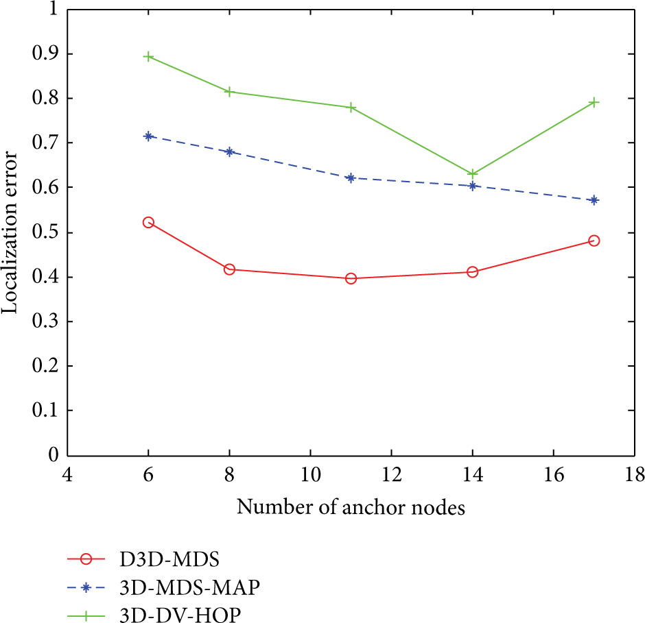
Localization error versus anchor nodes number.

The connectivity level of a network will affect localization accuracy too. We observe the localization error changes through varying the connectivity of the network. Simulation results show that the higher connectivity of the network can result in better performance in terms of accuracy as shown in Figure 4. The performance of proposed D3D-MDS scheme exceeds the other two algorithms when the network connectivity level is more than 14. It is expected as centralized range-free algorithms only perform well in regular topology. In our simulation scenario, the localization error of centralized algorithms mainly comes from the distance between two nodes which is obtained by the shortest path algorithms while proposed D3D-MDS uses clusters to decompose the network into regular shape and yields to good accuracy performance.

Figure 4

Localization error versus connectivity.

4.3. Time Complexity

The time consuming of the algorithms is relative to the computational complexity. Given n sensor nodes in a network and k anchors nodes, then according to the algorithm we know there are k clusters in the network. The time complexity of clustering algorithm is $O(n)$ . If the average number of sensor nodes in every cluster is $m\hspace{0.17em}\hspace{0.17em}(m=c/n)$ , the time complexity of computing the coordinates in every cluster is $O(k{m}^{\mathrm{3}})$ . The time complexity of merging the coordinates in different cluster is $O(n)$ , and that of transforming the relative coordinates to absolute coordinates is $O(n)$ too. The time complexity of our proposed D3D-MDS algorithm is $O(k{m}^{\mathrm{3}})$ . Compared with the time complexity of the 3D-MDS-MAP and 3D-DV-HOP, the time complexity decreases from $O(n^{\mathrm{3}})$ to $O(k{n}^{\mathrm{2}})$ . As shown in Figure 5, the consuming time of proposed algorithms can achieve approximately 100% improvements better than 3D-MDS and 50% better than 3D-DV-HOP with a relative big network size ( $n=\mathrm{800}$ ). Also Figure 5 shows that the consuming time increases with the network size. This is because a larger network consists of more clusters and thus requires more iterations to complete the localization process.

Figure 5

Time complexity.

4.4. Localization Rate

The proposed algorithm can fulfill partial localization in some extreme network topologies where other centralized algorithms may fail. Here the partial localization rate is described by the ratio of the number of nodes that can be positioned to all nodes. For example, we deployed 200 unknown sensor nodes randomly in a three-dimensional space shown as Figure 6. We carried out the simulation in case the network connectivity is 4.1179 and get that the partial localization rate is 53.4%. However, 3D-DV-HOP and 3D-MDS cannot locate the network when the network connectivity is lower than 8, and this feature can be clearly seen in Figure 7. We confirm that the partial localization rate has been improved via using our D3D-MDS algorithm. For example, when the network connectivity is lower than 7.6, our proposed algorithm has the localization rate between 42.45% and 100%, while the other two algorithms cannot execute the localization.

Figure 6

Partial localization.

Figure 7

Partial localization rate.

5. Conclusion

We present a new distributed method, D3D-MDS, for localization of wireless sensor networks regardless of topology. Our simulation results have shown that it can achieve low location errors and computational complexity, with high scalability to large-size wireless sensor networks. We also explore the influence of anchor nodes and connectivity on the algorithm. All these factors could affect the localization average error and location coverage of the algorithm. Simulation results show that our D3D-MDS is better than the other two algorithms mentioned in this paper, and it overcomes a series of difficulties in node identification, network decomposition, MDS computation, and global map reconstruction. All these are achieved in a way that is discrete, distributed, and low message and computation overhead. Future work may investigate proposed algorithm under more complicated irregular topology and explore the possibility using 3D localization results to facilitate data processing [28–30] in sensor networks.