Cluster-Based Architecture for Range-Free Localization in Wireless Sensor Networks

Abstract

In wireless sensor networks, the existing range-free localization techniques are based on either centralized approach or distributed approach. The centralized approach causes overhead, latency, and so forth, while the distributed approach is more complex. In order to overcome these issues, in this paper, we propose a cluster based architecture for range-free localization in wireless sensor network. Initially cluster-heads are selected based on the parameters such as link quality, residual energy, and coverage. An event based localization technique is applied to each cluster that involves straight line scanning of the clusters with deployed multiple sinks. The scanning process helps in estimating the location of target nodes with reference to the anchor nodes position. In case if any target node in the cluster is not localized, a distance based localization technique is executed that localizes the target node. By simulation results, we show that the proposed technique reduces the overhead and latency and increases the localization accuracy.

1. Introduction

1.1. Wireless Sensor Network

Wireless sensor network (WSN) consists of a large number of tiny wireless sensor nodes (often referred to as sensor nodes or, simply, nodes) that are typically densely deployed. Nodes measure the ambient conditions in the surrounding environment. These measurements are transformed into signals that can be processed to reveal some characteristics about the phenomenon.

The data collected is routed to special nodes, called sink nodes (also called Base Station, BS), in a multihop basis. Then, typically, the sink node sends data to the user via the Internet or satellite, through a gateway [1].

WSNs are emerging technology for monitoring the physical world. In a sensor network application, large numbers of tiny sensor nodes may be deployed and collaborate to gather data from the environment. Each node is equipped with a sensing modality, such as an image sensor, and has the capability to communicate over wireless channels. Such wireless sensor networks find applications in smart environments, surveillance, environmental monitoring, wildlife observation and tracking, and others [2].

1.2. Localization in Wireless Sensor Network

Localization in sensor networks can be defined as “identification of sensor node's position.” For any wireless sensor network, the accuracy of its localization technique is highly desired [3].

Localization refers to the ability of determining the position (relative or absolute) of a sensor node, with an acceptable accuracy. In a WSN, localization is a very important task; however, localization is not the goal of the network. In fact, localization is a fundamental service since it is relevant to many applications (target tracking, intruder detection, environmental monitoring, etc.), which depend on knowing the location of nodes. Localization is also relevant to the network's main functions like communication, geographical routing, cluster creation, network coverage, and so forth. Even collaboration typically depends on localization of nodes [1].

Localization algorithms for wireless sensor networks have been designed to find sensor location information, which is a key requirement in many applications of WSNs. A mobile anchor (MA) node cooperates with static sensor nodes and moves actively to refine location performance. Generally, based on the type of information required for localization, protocols can be divided into two categories (i) range-based and (ii) range-free protocols. Range-based techniques require special hardware for estimating the distance between anchors and sensors, which may become prohibitively expensive for large networks. Range-free techniques, on the other hand, do not impose such complexity as the anchor informs other sensors about its own position through message passing [4].

1.3. Limitations of Localization in Wireless Sensor Networks

• (1)

As wireless sensor network technology advances, acoustic source localization systems face new challenges. Wireless communication successfully deals with the spatial limitation of wired systems. Small-sized devices called “nodes” cooperate with each other for a common goal. The localization system must change its architecture and goals as the WSN system differs from the wired one [5].

(2)

The cluster-based acoustic source localization system has limitations when the system is actually deployed. The sensor nodes as well as the cluster-head are deployed uniformly. Topologically, the cluster should be located in the center of the sensor devices. The clustering-based systems have additional overhead for maintaining the clusters [5].

(3)

Sensor node consists of four basic components: sensing, processing, transceiver (transmitter and receiver), and power (usually, a battery) units. Recent advancements allow for the current generation of sensor nodes to become even smaller and cheaper. Consequently, nodes have reduced memory and processing capacities. It also has limited battery power. Moreover, due to a short transmission range (caused by restrained transmission power), nodes can only communicate with their local neighbors. A good localization solution must consider all these resource limitations and minimize the energetic, computational transmission, and hardware costs [1].

(4)

The network localization problem includes estimating the geographical location of all nodes in a network focusing on those nodes that do not have a direct way (e.g., GPS) to determine their own location.

(5)

Most localization algorithms are sensitive to the number of nodes and to the density of nodes (i.e., amount of localizing nodes per area unit) [1].

(6)

Some of the localization algorithms calculate the Euclidian distance between a pair of nodes by considering the shortest path between them. However, this is valid only when the shortest paths are similar to a straight line. In networks, where the deployed area has a concave topology, this is normally not valid, conducting to distorted results [1].

(7)

Some localization algorithms may not deal with localizing nodes, which are positioned in the limits of the WSN area. In this case, the distance information of each node is less and with lower quality because all the distance information belongs to the same side of the network [1].

(8)

Most of the proposed localization solutions have low accuracy in obstructed environments due to the existence of obstacles, which obstruct the line-of-sight between nodes (for instance, some nodes may not be able to see anchor nodes, which make localization unfeasible). Obstacles and terrain irregularities can also cause signal reflections, what leads to wrong distance estimations [1].

(9)

In most WSNs, nodes are stationary. As a result, most localization algorithms are designed specifically to this kind of networks. However, due to the emergence of new applications, algorithms should adapt to the existence of mobile nodes [1].

1.4. Clustering in Wireless Sensor Networks

Clustering is a standard approach for achieving efficient and scalable performance in wireless sensor networks. Clustering facilitates the distribution of control over the network and, hence, enables locality of communication. Clustering the nodes into groups saves energy and reduces network contention because nodes communicate their data over shorter distances to their respective cluster-heads. The cluster-heads forward the aggregated information to the base station. Only the cluster-heads need to communicate far distances to the base station. Clustering is a fundamental mechanism to design scalable sensor network protocols. A clustering algorithm splits the network into disjoint sets of nodes each centering on a chosen cluster-head. A good clustering imposes a regular, high-level structure on the network.

Many clustering protocols have been investigated as either stand-alone protocol or as a side effect of other protocol operations, for example, in the context of routing protocols or in topology management protocols. The majority of those protocols construct clusters where every node in the network is no more than one hop away from a cluster-head.

Clustering protocols themselves can be distributed or centralized. In centralized algorithm, a base node (usually sink node) collects information from network nodes and then partitions them into cluster. Therefore, one node forms clusters by global information that are gathered from the entire network. However, in distributed algorithm, each node runs algorithm independently by information about local neighbors [6].

1.5. Problem Identification

In [7], it is assumed that the optimal sink locations can be found using global information based method. We assume that the sinks have global knowledge; that is, every sink knows the geographical coordinates of the sensors and the other sinks. Now, as an extension to this work, we can do an effective localization technique for estimating the location information of sensors and sinks.

The existing works related to range-free localization are based on either centralized approach or distributed approach. The centralized approach faces limitations related to overhead, latency, and so forth, whereas the distributed approach suffers from problems related to high complexity. Hence, we propose a hierarchical architecture, which uses the advantage of both centralized and distributed architecture. As a result, the hierarchical architecture overcomes the limitations of the existing works.

Scanning entire network [8] will result in increased sequence order which may result in overhead and delay in the network. Thus, to overcome this problem, we propose a cluster-based architecture in wireless sensor networks for efficient localization of nodes. The usage of the anchor nodes within each cluster reduces the overhead and complexity in the network.

2. Related Work

Chen et al. [4] proposed a cooperative localization algorithm that considers the existence of obstacles in mobility assisted wireless sensor networks. In this scheme, a MA node cooperates with static sensor nodes and moves actively to refine location performance. The localization accuracy of this algorithm can be improved further by changing the transmission range of mobile anchor node. The algorithm takes advantage of cooperation between MAs and static sensors while, at the same time, taking into account the relay node availability to make the best use of beacon signals. For achieving high localization accuracy and coverage, a novel convex position estimation algorithm is proposed, which can effectively solve the localization problem when infeasible points occur because of the effects of radio irregularity and obstacles. This method is the only range-free based convex method to solve the localization problem when the feasible set of localization inequalities is empty.

Wang et al. [9] proposed a novel range-free localization algorithm using expected hop progress (LAEP) to predict the location of any sensor in a WSN based on an accurate analysis of hop progress with randomly deployed sensors and arbitrary node density. By deriving the expected hop progress from a network model for WSNs in terms of network parameters, the distance between any pair of sensors can be accurately computed. Since the distance estimation is a key issue in localization systems for WSNs, the proposed range-free LAEP achieves better performance and less communication overhead as compared to some existent schemes like DV-Hop and RAW. In addition, the effect of anchor placement on the algorithm performance by deriving the corresponding means position error range.

Zhou et al. [10] proposed a scalable localization scheme with mobility prediction (SLMP) for underwater sensor networks, by utilizing the predictable mobility patterns of underwater objects. In SLMP, localization is performed in a hierarchical way, and the whole localization process is divided into two parts: anchor node localization and ordinary node localization. During the localization process, every node predicts its future mobility pattern according to its past known location information and it can estimate its future location based on its predicted mobility pattern. Anchor nodes with known locations in the network will control the whole localization process in order to balance the tradeoff between localization accuracy, localization coverage, and communication cost.

Gopakumar and Jacob [11] proposed two novel and computationally efficient metaheuristic algorithms based on tabu search (TS) and particle swarm optimization (PSO) principles for locating the sensor nodes in a distributed wireless sensor network environment. Unlike gradient descent methods, both TS and PSO methods ensure minimization of the objective function without the solution being trapped into local optima. Further, a refinement phase with error propagation control for improvement of the results is implemented. The performance is compared with each other and against simulated annealing based WSN localization.

Zhou and Lamont [12] proposed an optimal local map registration algorithm for constructing global maps from local relative maps for wireless sensor network localization applications. Local maps are transformed into a global map using a set of affine transforms with each consisting of a rotation, a reflection, and a translation for each individual local map. The optimal transform is found by minimizing the discrepancies in the global map of the common sensor nodes shared by different local maps. A computationally efficient gradient projection algorithm is developed for finding the optimal transforms. The local map registration approach can solve many of the problems encountered by pairwise map merging based approaches and is able to achieve global optimal performance. It provides a systematic approach for constructing global maps from local maps.

3. Problem Identification and Proposed Solution

3.1. Overview

In this paper, we propose a cluster-based architecture for range-free localization in wireless sensor networks. In this technique, the clusters are formed using clique-covering algorithm and the cluster-head is selected based on the parameters such as link quality, residual energy, and coverage. An event based localization technique is applied to each cluster. It involves straight line scanning of the clusters with deployed multiple sinks. After performing the scanning process, node sequence is obtained that contains both anchor and target nodes. The position of the target nodes is determined with the help of anchor nodes. The cluster-head maintains the location information of target nodes. If any target node within the cluster is not localized, then a distance based localization technique is executed.

3.2. Estimation of Metrics

3.2.1. Similarity Measure Estimation

The time-ordered data sequence at each sensor node forms a time series. The estimation of similarity of the two time series involves the following three cases.

The data values of two sensor nodes $N_i$ and $N_j$ are said to be similar, if

• (i)

$\text{m}{\text{t}}_i=\text{m}{\text{t}}_j$ ,where ${\text{mt}}_i$ and ${\text{mt}}_j$ are the magnitudes of the values of $N_i$ and $N_j$ ,

(ii)

$D_{ij}<D_{\text{th}}$ ,where ( $D_{ij}$ ) is the distance between $N_i$ and $N_j$ and $D_{\text{th}}$ is distance threshold,

(iii)

${\delta }_R<{\delta }_{\min }$ , ${\delta }_R\text{ABS}(R_j-R_i)$ ,where $R_i$ and $R_j$ are the sending rates of $N_i$ and $N_j$ , respectively, given by

$$\begin{array}{cc}& R_i=\frac{N{P}_i}{T},\\ R_j=\frac{N{P}_j}{T}.\end{array}$$

(1)

Here NP is the number of packets sent in a time period T.

${\delta }_R$ is the absolute difference of $R_i$ and $R_j$ and ${\delta }_{\min }$ is the minimum threshold value for ${\delta }_R$ .

We can represent the two nodes as points in 3 dimensions. Node i has coordinate ( $\text{m}{\text{t}}_i$ , $D_i$ , and $R_i$ ) and Node j has coordinate ( $\text{m}{\text{t}}_j$ , $D_j$ , and $R_j$ ). Similarity measure (SM) between the two nodes is based on these coordinates. In order to estimate the similarity measure for these two nodes, the Euclidean distance is used. The Euclidean distance between the nodes $N_i$ and $N_j$ is given by [13]

$$\begin{array}{cc}& \text{S}{\text{M}}_i=\sqrt{{{\displaystyle \sum }}_{k=\mathrm{1}}^n{\left(x_{ik}-x_{jk}\right)}^{\mathrm{2}},n=\mathrm{3}}.\end{array}$$

(2)

Here,

$$\begin{array}{cc}& x_{i\mathrm{1}}=\text{m}{\text{t}}_i,\hspace{1em}\hspace{1em}{x}_{i\mathrm{2}}=D_i,\hspace{1em}\hspace{1em}{x}_{i\mathrm{3}}=R_i,\\ x_{j\mathrm{1}}=\text{m}{\text{t}}_j,\hspace{1em}\hspace{1em}{x}_{j\mathrm{2}}=D_j,\hspace{1em}\hspace{1em}{x}_{j\mathrm{3}}=Rj.\end{array}$$

(3)

3.2.2. Estimation of Residual Energy

The residual energy ( $E_{\text{res}}$ ) of each node ( $N_i$ ) after one data communication is estimated using [14]

$$\begin{array}{cc}& E_{\text{res}}=E_i-\left(E_{\text{tx}}+E_{\text{rx}}\right),\end{array}$$

(4)

where $E_i$ = initial energy of the node and $E_{\text{tx}}$ & $E_{\text{rx}}$ = energy utilized at the time of transmission and reception of data.

3.2.3. Estimation of Link Quality

Link quality indicator is defined as the characterization of strength and/or the quality of a received packet. It is directly proportional to received signal strength (RSSI). Its value varies from 0 to 255:

$$\begin{array}{cc}& \text{LQ}\alpha \text{RSSI}.\end{array}$$

(5)

RSSI is the ratio of the received power ( $P_{\text{rx}}$ ) to the reference power ( $P_r$ ). In general, $P_r$ is equivalent to absolute value, say, 1 mW:

$$\begin{array}{cc}& \text{RSSI}=\mathrm{10}·\log \left(\frac{P_{\text{rx}}}{P_{\text{ref}}}\right)\left(\text{dBm}\right).\end{array}$$

(6)

When $P_{\text{rx}}$ increases, then RSSI value is also increased which in turn enhances the link quality [15].

3.2.4. Estimation of Node Coverage

The node coverage ( $C_n)$ is estimated based on the relative node speed and node degree using

$$\begin{array}{cc}& C_n=\left(\alpha *z_i\right)+\left(\beta *D_{n_i}\right),\end{array}$$

(7)

where $z_i$ is relative speed of the node, $D_{n_i}$ is node degree, and α and β are constants.

In the above equation, $z_i$ is determined based on the distance among the nodes at time t and the $D_{n_i}$ is related to the direct wireless link among the nodes at time t.

3.2.5. Estimation of Distance

The distance among the sensor nodes is defined as the product of transmission range and corresponding hop counts [9]. It is given using

$$\begin{array}{cc}& D=\gamma *\text{HC},\end{array}$$

(8)

where γ is transmission range and HC is hop count among the nodes.

3.2.6. Clique-Covering Algorithm

The clustering problem can be represented as a clique-covering problem. A graph G is created such that each sensor node is a vertex in the graph. An edge ( $u,v$ ) is drawn if $\text{DM}(u,v)\le {\text{DM}}_{\text{thr}}$ . In the graph, we can observe that a cluster is a clique. The clique-covering problem does not even allow constant approximation and it is proven NP-complete. In order to gain a rough approximation, we can use a greedy algorithm. In order to cover more vertices, which have not been clustered, this algorithm heuristically finds the cliques. Until all vertices are covered, the search starts from the vertex with the largest degree. The output of this algorithm is a set of cliques that cover all vertices. The clique-covering algorithm is as Algorithm 1.

Algorithm 1

(1) Let {UV} be the set of all uncovered vertices.

(2) While $\left\{\left\{\text{UV}\right\}\ne \mathrm{\Phi }\right\}$

(2.1) Choose $\mathrm{\upsilon }\in \{\text{UV}\}$ such that $\text{ND}(\mathrm{\upsilon })=\max \{\text{ND}(i)\}$

   Where ND represents the Node Degree

(2.2) Let $N(v)$ is the set of neighbors of V

(2.3) Add N(v) to {SV}

(2.4) Create graph $T_{\text{graph}}=\{\text{SV}\}$

(2.5) Find $\text{ND}(j)$ , $\forall j\in T_{\text{graph}}$

(2.6) Sort {SV} in descending order of ND(j)

(2.7) Construct a clique $C=\{\mathrm{\upsilon }\}$

(2.8) While $\left\{\left\{\text{SV}\right\}\ne \mathrm{\Phi }\right\}$

(2.8.1) Choose next vertex $k\in \{\text{SV}\}$

(2.8.2) If $N\left(k\right)=i\hspace{0.17em}\hspace{0.17em}\forall i\in \{\text{SV}\}$ , then

(2.8.2.1) Add k into C

(2.8.3) End if

(2.9) End while

(2.10) Return C

3.3. Clustering Algorithm

This algorithm involves the analysis of the data generation rate and the similarity between data series by the sink (estimated in Section 3.2.1) and grouping of nodes into various clusters. In each cluster, the cluster-heads are selected based on the residual energy, link quality, and node coverage (estimated in Sections 3.2.2–3.2.4). The steps involved in the clustering algorithm are as follows.

(1) Each sensor node ( $N_i$ ) transmits the data to the sink ( $S_i$ ) with the specified data rate.

(2)   $S_i$ receives the data from each sensor node.

(3)   $S_i$ estimates the similarity measure SM (by (2)).

(4) If $\text{SM}>{\text{SM}}_{\text{th}}$ , where SM_th is the similarity threshold,

Then

Add these nodes in a cluster (Using Clique Covering Algorithm Shown in Section 3.2.6) Nodes within the cluster with $E_{\text{res}}$ , LQ, and $C_n$ greater than threshold are chosen as cluster-head.

End if

(5)   $S_i$ stores the details of all the $\text{CH}s$ and their data structures and broadcast cluster information packet ( $\text{C}\_\text{IN}$ ) to all the $\text{CH}s$ :

$$\begin{array}{cc}& S_i⟶\text{CH}s:{\text{C}}_{-}\text{IN}.\end{array}$$

(9)

The $\text{C}\_\text{IN}$ includes the cluster-heads ID and its position. $\text{CH}s$ stores the $\text{C}\_\text{IN}$ in its cluster table.

Figure 1 describes the cluster formation architecture. The architecture includes the cluster members, cluster-head, anchor nodes, and sink.

Figure 1

Cluster architecture.

3.4. Event Based Localization Technique

Consider a clustered sensor network with X target nodes and Y anchor nodes.

•  

Let q represent the number of scans.

 

Let n be the number of parts.

 

Let $L_{{\text{an}}_i}$ be the location of anchor nodes.

 

Let p be the slope of the line.

 

Let v be the number of anchor nodes.

We utilize the multisequence positioning (MSP) technique that scans the cluster area from different directions using two straight lines. Each scan is treated as events. After scanning process, the sequential list of nodes that detects the events is obtained. The sequence contains both anchor nodes and target nodes. In addition, in order to minimize the power consumption, multiple sinks are deployed [16]. The clusters $C_1$ , $C_2$ , and $C_3$ communicate their information to sink $S_i$ . Similarly, $C_4$ and $C_5$ communicate their information to sink $S_j$ . For simplicity, the localization related to clusters $C_1$ , $C_2$ , and $C_3$ is demonstrated below.

For example, consider Figure 2. The vertical scan in $C_1$ , $C_2$ , and $C_3$ obtains the following node sequence:

•  

$C_1:\{N_1,N_2,N_4,N_3\}$ ,

 

$C_2:\{N_{10},N_{11},N_{13},N_{14},N_{12}\}$ ,

 

$C_3:\{N_5{N}_6{N}_7{N}_9{N}_8\}$ .

Figure 2

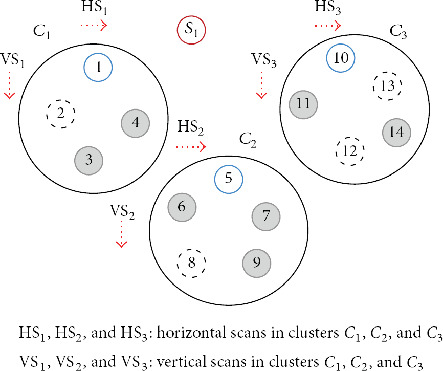
Scanning event.

The horizontal scan in $C_1$ , $C_2$ , and $C_3$ obtains the following node sequence:

•  

$C_1:\{N_2,N_1,N_3,N_4\}$ ,

 

$C_2:\{N_6,N_8,N_5,N_7,N_9\}$ ,

 

$C_3:\{N_{11},N_{10},N_{12},N_{13},N_{14}\}$ .

As the locations of the anchor nodes are available, the anchor nodes in the two node sequences actually split the area horizontally and vertically of the clusters into n parts. The number of parts is the function of the number of anchor nodes, the number of scans, the anchor nodes location, and slop of each scan line:

$$\begin{array}{cc}& n:f\left\{v,q,L_{{\text{an}}_i,}p\right\}.\end{array}$$

(10)

For X anchor nodes, q scans are performed from different angles, obtaining q node sequences and dividing the cluster area into many small parts. This is achieved using “Pie Cutting Theorem.” This theorem helps in splitting the cluster area into O( $X^2{q}^2$ ) parts.

If X and q is large,

Then

Target node area becomes small and

Location of target node can be achieved more accurately.

End if

This reveals that the accurate estimation of target node is affected by the anchor nodes as well as the number of scan events.

Following the processing of node sequence, for each cluster, the boundaries are obtained. Based on the newly obtained boundaries, the cluster area shrinks. Finally, the centroid is estimated that fixes the centre of gravity of the target node area, thus estimating the location of the target node ( $L_{\text{tn}}$ ). The cluster-head maintains the localized target nodes information in its member table, which includes the target node id and its location information.

3.5. Distance Based Localization Technique

If any target node within the cluster is not localized, then a distance based localization technique is executed that allows localizing the nonlocalized nodes. The algorithm describing the distance based localization technique is given in Algorithm 2.

Algorithm 2

(1) Initially the localized target node ( ${\text{TN}}_i$ ) broadcast a distance discovery packet (Dist_Disc) to every

  other node in the cluster ( $N_i$ ).

             ${\text{T}{\text{N}}_i}^{\mathrm{*}}\to N_i:\text{Dist\_Disc}$

(2) Dist_Disc packet travels along the cluster to estimate the distance (Described in Section 3.2.4) in

   terms of number of hops among the nodes.

(3) Each node keeps the record of Dist_Disc packet using counter.

(4) The estimated distance allows localizing the nodes.∖

(5) Following the localization, the node transmits the localized nodes information to its cluster head.

   The cluster head updated the information in its cache.

(6) When any $N_i$ wants to find the location of a ${\text{TN}}_i(L_{{\text{TN}}_i})$ , it transmits a Location request message

   (L_req) to its cluster head ( ${\text{CH}}_i$ ).

             $N_i\to \text{C}{\text{H}}_i:L\text{\_req}$

${\text{CH}}_i$ (say Home ${\text{CH}}_i$ ( ${\text{HCH}}_i$ )) upon receiving L_req message, verifies its member table for the target

node.

   If ${\text{TN}}_i$ found

   Then

    $N_i\leftarrow \text{HC}{\text{H}}_i:L_{{\text{TN}}_i}$

   Else

${\text{HCH}}_i$ broadcasts L_req to all other $\text{C}{\text{H}}_i$ existing in the cluster table.

If ${\text{TN}}_i$ found

Then

          $\text{C}{\text{H}}_i\to \text{HC}{\text{H}}_i:L_{{\text{TN}}_i}$

          $\text{HC}{\text{H}}_i\to N_i:L_{{\text{TN}}_i}$

   End if

   End if

This reveals that once the target node is found in the home ${\text{CH}}_i$ itself, then the location information of the target node is transmitted directly to requested node. Else, the search is performed in all other ${\text{CH}}_i$ existing in the cluster table and the location of the target node is obtained.

Advantages of This Approach

• (1)

As the computation is done clusterwise, the problem of scanning entire network, which may result in increased sequence order, can be avoided.

(2)

This technique does not require any costly hardware and requires only a small number of anchor nodes. So, high localization accuracy can be achieved economically by introducing more events instead of more anchors.

(3)

Multiple sink deployment reduces power consumption.

4. Simulation Results

4.1. Simulation Parameter

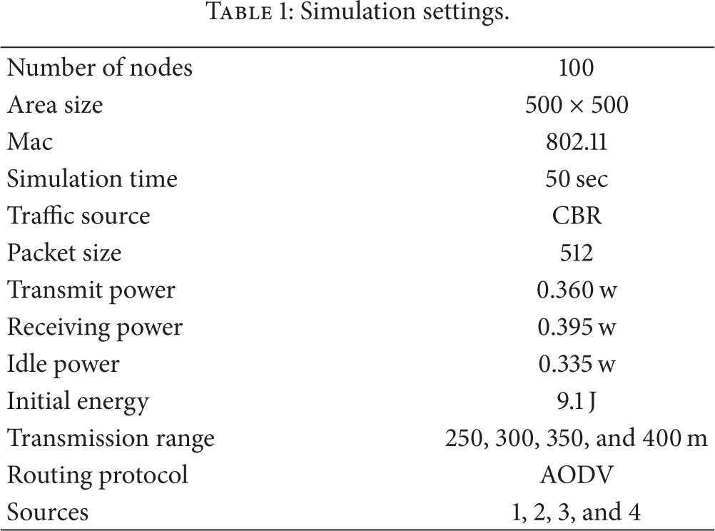
The cluster-based architecture for range-free localization (CBA) is evaluated through network simulator (NS2) [13]. We use a bounded region of 500 × 500 m², in which 100 sensor nodes are randomly placed and two sink nodes are located in the network. The power levels of the nodes are assigned such that the transmission range and the sensing range of the nodes are all 250 meters. In the simulation, the channel capacity of mobile hosts is set to the same value: 2 Mbps.

The simulated traffic is constant bit rate (CBR). The simulation topology is given in Figure 3.

Figure 3

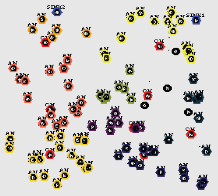
Simulation topology.

Table 1 summarizes the simulation parameters used.

Table 1

Simulation settings.

Number of nodes	100
Area size	$\mathrm{500}\times \mathrm{500}$
Mac	802.11
Simulation time	50 sec
Traffic source	CBR
Packet size	512
Transmit power	0.360 w
Receiving power	0.395 w
Idle power	0.335 w
Initial energy	9.1 J
Transmission range	250, 300, 350, and 400 m
Routing protocol	AODV
Sources	1, 2, 3, and 4

4.2. Performance Metrics

The performance of our proposed CBA technique is compared with the expected hop progress (EHP) [9] method and scalable localization scheme with mobility prediction (SLMP) [10]. We evaluate mainly the performance according to the following metrics.

Average Energy Consumption. This is the average energy consumed by the nodes in receiving and sending the packets.

Packet Delivery Ratio. It is defined as the number of data packets received successfully with the total number of packets sent.

Average End-To-End Delay. It includes the localization delay, tracking delay, and transmission delay.

Localization Error. It is the difference between the estimated and actual locations of the nodes.

The time complexity of CBA involves cluster formation and cluster-head election time by the sink which is comparatively less when compared to the EHP and SLMP techniques where the localization has to be applied for the whole network.

4.3. Results

4.3.1. Results Based on Range

The transmission range is varied as 250,300,350 and 400 m/s and the above performance metrics are measured for all the 3 schemes.

Figure 4 shows the delay occurred for all the 3 schemes, when the transmission range is increased. The increase in transmission range results in the increase of delay, since more nodes have to be localized. From the figure, we can see that the delay of CBA is 28% less than EHP and 14% less than SLMP, since CBA uses the clustered architecture for performing localization.

Figure 4

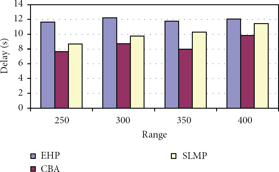
Range versus delay.

Figure 5 shows the packet delivery ratio of all the 3 schemes, when the transmission range is increased. It can be seen that the delivery ratio of CBA is 30% higher than EHP and 5% higher than SLMP. This is due to the fact that CBA has the features of cluster-based power efficient scheduling architecture for efficient delivery of data.

Figure 5

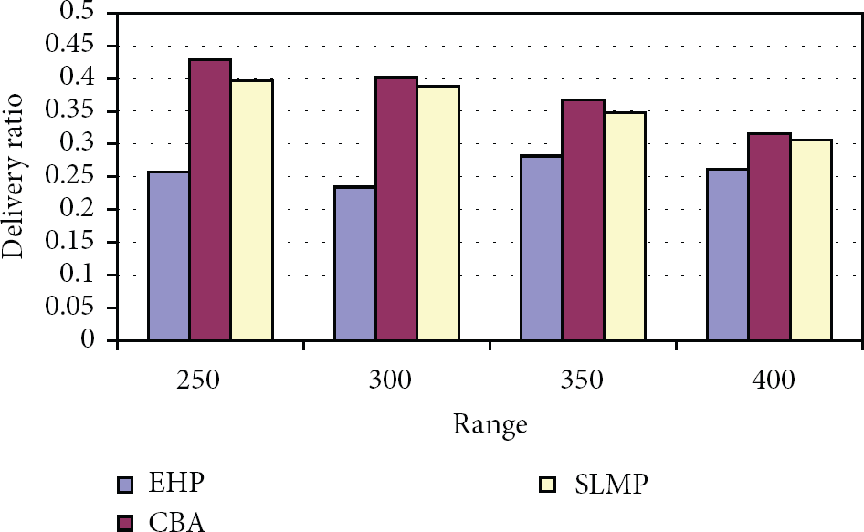
Range versus delivery ratio.

Figure 6 shows the average energy consumption of all the 3 schemes, when the transmission range is increased. From the figure, we can see that CBA has 9% and 3% reduced energy consumption when compared to EHP and SLMP, respectively, since CBA has cluster-based duty-cycle scheduling to reduce the transmission power.

Figure 6

Range versus energy consumption.

Figure 7 presents the estimation error for all the 3 schemes, when the transmission range is increased. The error increases linearly, as the range increases. From the figure, we can see that the estimated error of CBA is 24% less than EHP and 7% less than SLMP, since the localization is performed by each cluster-head in parallel, the accuracy will be more.

Figure 7

Range versus estimation error.

4.4. Results Based on Sources

Here, the number of sources per cluster is varied from 1 to 4.

Figure 8 shows the delay occurred for all the 3 schemes, when the number of sources is increased. The increase in sources results in the increase of delay, since more nodes have to be localized. From the figure, we can see that the delay of CBA is 37% less than EHP and 14% less than SLMP, since the localization is performed by each cluster-head in parallel, the delay will be less.

Figure 8

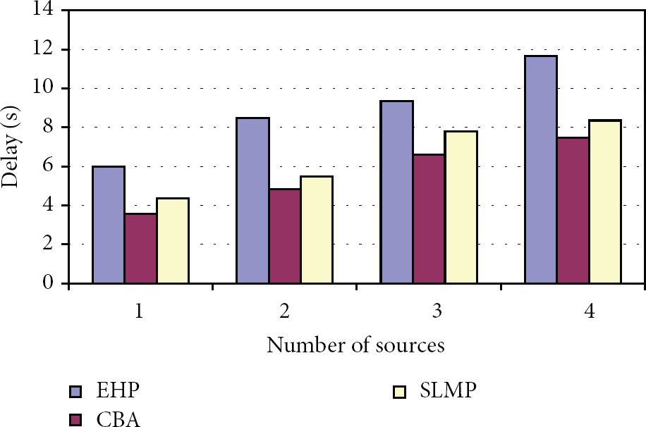
Number of sources per cluster versus delay.

Figure 9 shows the average energy consumption of all the 3 schemes, when the number of sources is increased. From the figure, we can see that CBA has 8% and 5% reduced energy consumption when compared to EHP and SLMP, respectively, since CBA has cluster-based duty-cycle scheduling to reduce the transmission power.

Figure 9

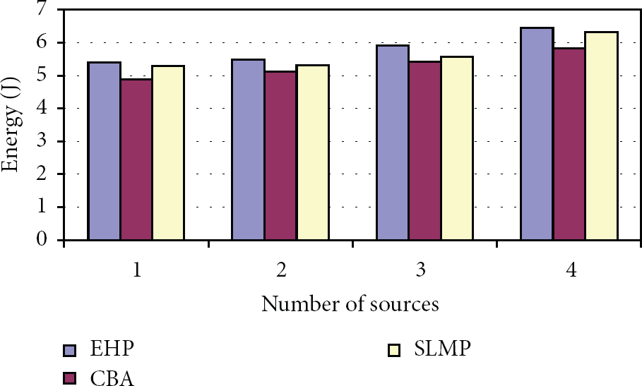
Number of sources per cluster versus energy consumption.

From the simulation results of both sections, we can conclude that CBA significantly outperforms EHP and slightly outperforms SLMP.

5. Conclusion

In this paper, we have proposed a cluster-based architecture for range-free localization in wireless sensor network. Initially, the cluster-heads are selected based on the parameters such as link quality, residual energy, and coverage. An event based localization technique is applied to each cluster that involves straight line scanning of the clusters with deployed multiple sinks. The scanning process helps in estimating the location of target nodes with reference to anchor nodes position. In case if any target node in the cluster is not localized, a distance-based localization technique is executed that localizes the target node. By simulation results, we have shown that the proposed technique reduces the overhead and latency and increases the localization accuracy.