
Abstract
The analysis two-phase flow inside centrifugal pumps is a fundamental issue in several engineering applications. This often represents a bad working condition with respect to single phase one, causing head reduction, efficiency decrease, and higher operational costs in terms of energy and money. The paper reports a numerical analysis of bubbles behavior inside centrifugal pumps. Equations regulating the air bubble motion within the rotor of a centrifugal pump have been solved considering the effects of all forces acting. Coalescence phenomena have been investigated too, in order to identify how gas zone presence in the rotor can lead to anomalous working condition. Results are reported in graphs and diagrams varying bubble dimension and water flow rate. An experimental approach to visualize the two-phase flow field inside the impeller is presented too. Images have been acquired, elaborated, compared with numerical results, and discussed in order to understand the interaction between gas phase and liquid phase and to correlate this behavior with the energy dissipation phenomena for a centrifugal pump.
1. Introduction
The analysis of bubbles behavior inside centrifugal pumps is a fundamental issue in several engineering applications. This often represents a bad working condition with respect to single phase one, causing head reduction, efficiency decrease, and higher operational costs in terms of energy and money. Moreover, when gas fraction becomes too high, a gas locking condition is reached, when pump flow rate falls down to zero, and pump doesn't pump.
Petroleum production and nuclear plants are the most typical situation where two-phase flow can occur within centrifugal pumps. In the first case electrical submersible pumps (ESP) show head decrement due to slippage, that is, a difference between gas and liquid velocities. In the last case, for example, in loss of fluid conditions, stream pressure goes down and a two-phase mixture is generated during expansion. In particular in nuclear plants, such as PWR, loss of coolant accident (LOCA) is very dangerous because of liquid radioactivity. The behavior of pumps working with two-phase flow generated by accidental conditions must be studied in order to know pumps limits in anomalous conditions and in order to design pumps that are suitable for working in anomalous conditions.
Another typical situation where two-phase flow can occur is related to geothermal plants exploiting hot water with a considerable content of noncondensable gas, like carbon dioxide, nitrogen, and oxygen.
Several studies are reported in literature dealing with this topic, often based on major assumptions, neglecting the bubble effect on pressure field or liquid phase velocity, moreover, regardless to possible bubble fragmentation or coalescence phenomena.
One of the first studies was performed numerically and experimentally by Schrage and Perkings [1], considering the single bubble motion in a rotating annulus, subject to buoyancy, virtual mass, and drag forces, and neglecting bubble interaction. Experimental results showed a satisfactory agreement with numerical results.
Other studies followed by Runstadler [2], Mikielewicz et al. [3], Grison and Lauro [4], and Minemura and Murakami [5] give correlation between the most significant parameters of two-phase flow in pumps.
A further and more detailed analysis of air bubbles motion within a centrifugal pump rotor was performed by Minemura and Murakami [6] taking into account five different forces effects:
slippage (drag force due to velocity gap between air and water),
pressure gradient forces (around the bubble),
forces by density gap between two phases,
virtual mass effect,
Basset force.
They found that two of these actions mostly influence bubble motion: slippage and pressure gradient. The bubbles deviate from liquid streamlines and deviation increases with bubbles diameter. Such trends were in good agreement with experimental results.
Afterwards Sterret et al. [7] applied a similar method to two different impeller configurations: radial vane and logarithmic spiral. They found that bubble diameter has a key role in its motion and trajectory through the vane and there is a maximum bubble diameter for which the bubble can exit the vane.
Within experimental investigations, Lea and Bearden [8] examined different centrifugal pumps in various pressure and flow rate conditions, highlighting that flow rate, suction pressure, and gas void fraction (GVF) mainly affect pump performances. In particular they found that pump head drop increases with GVF.
Cirilo [9] came to the same conclusions, attributing pump performance degradation to gas accumulation in the impeller.
Until today biphasic performances of centrifugal pumps are not well predictable by theoretical methods due to the following weaknesses.
The effect of suction pressure is overlooked.
Only GVF <10% are considered, while often this value is passed.
Slip factor of two-phase flow is considered the same as for single phase.
The physical phenomenon which causes head degradation is not well clear.
About pump operation in nuclear plants, Poullikkas [10, 11] examined the effect of two-phase flow on the reactor cooling pumps, while Caridad et al. [12] treated similar pump problems in petroleum production plants.
In the last years a lot of CFD applications have been developed about centrifugal pumps, especially in anomalous working conditions, as reported by Shah et al. [13].
Generally it is possible to understand what is the global behavior of the two-phase flow but not yet which is the real distribution of the gas phase inside the mobile ducts and how the flow field changes relating to the gas phase distribution. An experimental analysis, as reported in Amoresano et al. [14] and Zhu et al. [15], is a basic tool to better realize the physical phenomenon and validate numerical results of models application.
This paper reports a numerical and experimental analysis of two-phase flow inside centrifugal pumps. Equations regulating the air bubble motion within the rotor of a centrifugal pump have been solved considering the effects of all forces acting. Bubble coalescence phenomena have been investigated too, by a numerical approach, analyzing the mechanism that forms the interface surface between water and gas (in this case air) inside the impeller.
By an experimental approach the two-phase flow field inside the impeller is visualized in order to understand the interaction between gas phase and liquid phase and to correlate these behaviors with the energy dissipation phenomena for a centrifugal pump.
2. Numerical Approach
2.1. Bubble Motion
Multiphase flow (particularly mixture of liquid and gas bubbles) may occur in pumping processes through the chamber between the casing wall and the rotating impeller. Due to difference in densities of the bubbles and the liquid fluid that is being pumped, the bubbles move differently in the flow, namely, towards the low-pressure zone in the chamber. The performance of the pump goes down with the increase of bubbles in the chamber.
In all such phenomena, there is relative motion between bubbles on one hand and surrounding fluid on the other. In many cases, transfer of mass and/or heat is also of importance.
Often the dispersed phase is treated using the Lagrangian approach by tracking its trajectory along which the information is passed [16].
In the following study, the equations governing the bubble motion through the rotor vans of a centrifugal pump have been written and solved. As reported in Figure 1, rotor blades are in radial configuration although backslope blades are more widely used in such pump. This configuration has been chosen as a first approach in order to simplify the numerical simulation and to verify its agreement with experimental results. No axial inducer section has been adopted.

Cylindrical coordinates for the bubble motion analysis.
The following hypotheses have been adopted:
small diameter of the bubble,
water in steady flow,
not compressible and not viscous fluid.
The analysis has been set up in cylindrical coordinates as shown in Figure 1.
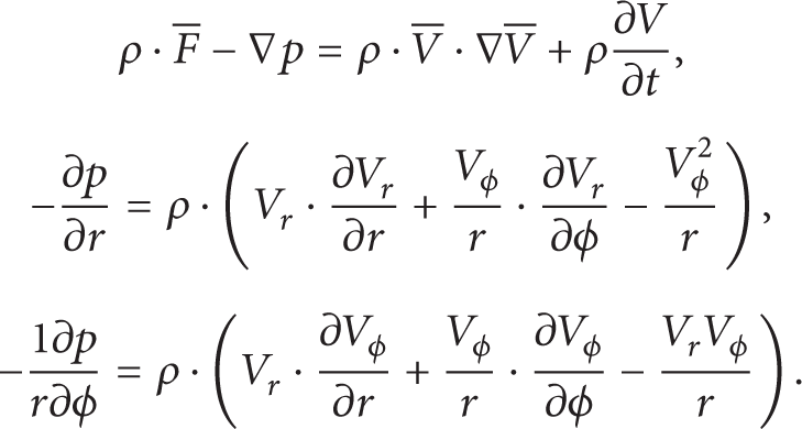
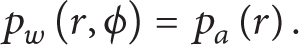
Euler equation for water flow is

where W represents the water velocity, p water pressure, and ω the angular velocity of the rotor.
Once known the motion field, by Euler equation integration, it is possible to determine the pressure distribution within the single rotating duct of the impeller. In other words from W r (r,φ), Wφ(r,φ) and W z (r,φ) functions, the pressure function p(r,φ) can be derived.
Assuming the following water motion field:

the pressure distribution can be formulated as follows:

About bubble motion a small number of bubbles have been considered, so the water motion can be assumed to be not altered by bubble presence. Moreover no mass and heat transfer between water and bubble has been taken into account. The force balance on the bubble can be written as

where M and V indicate mass and velocity of the bubble. The air mass in the bubble can be evaluated by applying the perfect gas law, using the pressure value achieved by water motion. The forces considered are, respectively, the drag force, the pressure gradient force, the body force, the water inertia force, and the Basset force, as defined by Minemura and Murakami [6].
Taking into account the forces expressions, it can be written as

where drag coefficient C d can be evaluated by Reynolds number [17] and virtual mass coefficient C v is assumed to be 0.5 as for a spherical droplet [17].
Starting from forces balances, bubble motion equations have been derived and solved by time discretization, assuming Δt = 10−6 sec.
Once assigned initial position and velocity of the bubble, acceleration can be calculated and so can the position and velocity at the subsequent time step. Initial bubble condition must be carefully chosen: r will be equal to internal radius of the impeller while the angular position φ will be included between 0 and α, where α = 360°/number of blades.
About velocities at rotor inlet, we assumed, both for water and bubble, Vφ0 = Wφ0 = 0; moreover, bubble has been considered to have the same velocity of water at impeller inlet Vr0 = Wr0.
Bubble diameter is updated step by step by

applicable all along trajectory.
Applying this model it is possible to characterize the single bubble motion and diameter reduction.
2.2. Coalescence
Furthermore a fundamental phenomenon occurring into rotor van is the coalescence of bubble, generating a gas phase volume. In order to evaluate bubble coalescence phenomena, a numerical approach has been adopted analyzing the mechanism that forms the interface surface between water and gas (in this case air) inside the impeller.
The basic hypotheses of this theory are:
perfect fluids,
body forces negligible,
steady angular velocity,
steady temperature,
periodic regime,
rectangular blade.
Starting from vector Euler's Equation in cylindrical coordinates and taking into account hypotheses 2, 3, and 6 the following equations can be formulated:
Integrating these two equations, pressure field can be evaluated in two extreme cases: only water inside the impeller and only gas inside the impeller.
(i) Water Phase. The velocity components related to the hypothesis are

and V e is derived by
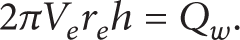
Substituting the integration of this system gives
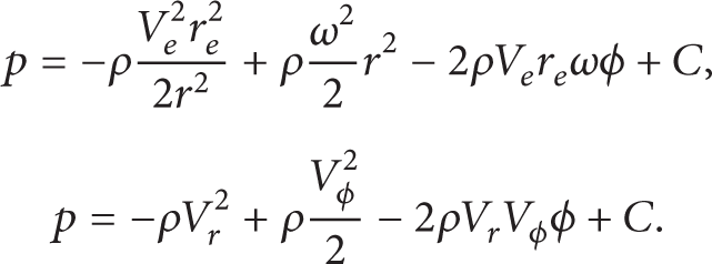
The integration of these two equations between two sequential blades gives
C is calculated by the following limit condition:

(ii) Gas Phase. It is possible now to integrate the gas phase. In this case we consider only the presence of gas phase inside the impeller.
Applying the Euler's equation and taking in account the new variable ρ and applying the perfect gas equation, the ρ function will be

In this way we can write

According to the hp. 4 (T = const)

It is now possible to solve pressure field only for the gas phase inside the impeller. Inside it only the gas phase exists and it remains inside.
So the equation of the velocity will be

and pressure gradients will be

The description of the entire pressure field in the gas phase is given by:

If ω = 0⇒C2 = pa0.
The pressure field in this case is described by
3. Experimental Analysis
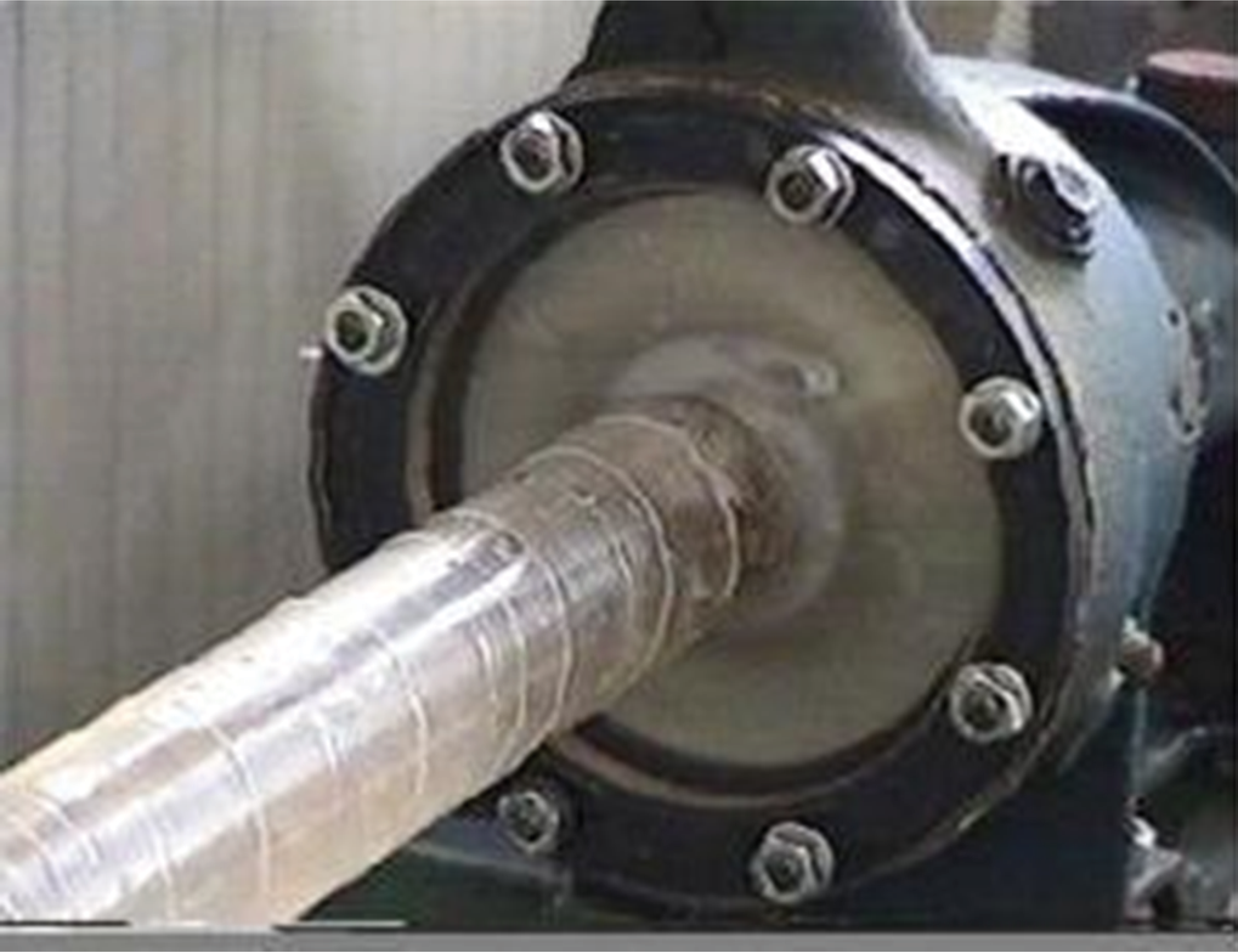
Experimental apparatus is made of a centrifugal pump with suction duct and flange, both transparent, as shown in Figure 2, in order to allow flow visualization by a CCD camera at high frame acquisition rate. A quoted sketch of the rotor is reported in Figure 3.
Centrifugal pump with suction duct and flange, both transparent.

Dimensioned sketch of the rotor.
Flow visualization is performed along the transparent duct and inside the impeller, in the first case in order to study which are the flow field characteristics in the stationary case and, in the second case, in order to define the distribution of the gas phase.
Pump is driven by an electrical motor with inverter regulation. Hydraulic circuit is switchable to two different heads and has a bypass regulation too. All facility components are reported in Figure 4.

Experimental apparatus.
The dissipation phenomena are quantified by the balance at electrical motor. The amplitude of the rotation around the zero value of the rotation axis gives important relationship with the quantitative presence and permanence of the gas phase inside the impeller.
In the preliminary tests, only water has been pumped within the hydraulic circuit, in order to know pressure, temperature of the water inside the impeller, and temperature of the external environment. In this way it was possible to map the characteristic lines of the pump, changing the rpm (head versus flow rate). The characteristic values like the rpm value, volumetric flow rate and mass flow rate, drop pressure between the inlet and the outlet of the impeller, and the medium value of the torque soaked from the rotor were recorded. For each condition of the rpm regime these parameters were evaluated to understand the real flow dynamics characteristics of the impeller, that is, the triangles of velocity, NPSHA(R), and so forth. In the second phase a known percentage of gas was injected inside the duct or tracing particles. In this way it was possible to fix a controlled mode of the particular two-phase flow and analyze it.
In the first step a little amount of gas was injected in the way to produce only one bubble having a volume of 5 × 10⁻⁵ m3. This volume of air goes on until it arrives on the upper side of the duct near the inlet section of the pump. Immediately before the inlet section the two-phase flow is clearly separated: the gas phase will be up and the liquid phase down.
The flow dynamics model of the radial impeller will surely be changed. In fact the pump works with two stratified phases. The configuration of the new flow field is showed in a typical frame recorded with the high velocity CCD camera and reported in Figure 5.
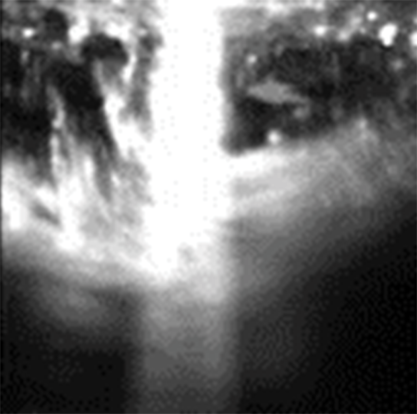
Separation inside a moving duct between air and water in slug flow.
It is possible to see that inside the impeller gas and liquid phase is still separated too. Really it is possible to have some kinds of behavior of the pump changing the air flow rate inside the region of the slug flow.
4. Image Elaboration
The geometric parameters are acquired by a visualization [18] technique. The system is able to acquire, by a fastcam CCD, images with frame rate of 10.000 frame/s. In this way it is possible to acquire image sequences in order to follow the phenomena evolution versus time.
The Nyquist-Shannon theorem has been considered to avoid aliasing effects in time sequence image acquisition [19–21]. The angular velocity is acquired by magnetic transducer giving the tachometric reference necessary for the image sequence definition. The technique of measurement of very small geometric entities, like diameters or grooves, needs a specific camera device with MACRO objective. Particular attention is paid to the source light to avoid its intensity variations affecting the measurement. A bright light source powered 12/24 V DC stabilized has been chosen to minimize the shadows and the light spikes due, respectively, to the instantaneous absorbance and reflection. The ambiguity due to light diffusion has been minimized maximizing the image contrast between the blade profile, treated with white absorbent paint, and the mobile duct treated with black absorbent paint.
The recorded images must be treated offline with specific digital image processing to recover correct information starting from the raw files containing all the frequencies, noise included. The images clearly show the presence of two phases and the aim of this paper is to border the gas phase from the liquid one. This is possible because the energy balance of the diffuse light has different distribution when impressing on a gas or a liquid phase. In this analysis the correct definition of the border lines between the two phases has an important weight. The CCD camera provides a digital image and, of course, the border lines can be affected by approximation due to pixel representation. An “ad hoc” logical procedure has been developed to extract the correct contours.
“In primis,” it is necessary to define the “neighbourhood system.”
For a grid the dth neighbour level N ij d , for any element (i,j) is defined like

with
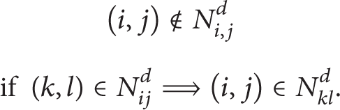
When d = 1

It can be obtained taking 4 boundary pixels like in Figure 6.

Neighborhood system N d .
In Figure 7 a schematic representation of the procedure is shown. In it, there are 3 layers.

Schematic representation of layers hierarchy.
In each of them there will be M × N neurons (assuming an M × N image). Each neuron corresponds to one pixel. Among the in/out layers there are a number of layers > 0. Neurons belonging to the same level have no connection among them. Each neuron in a layer is connected to the corresponding neuron in the previous layer and its neighboring neurons; each neuron, in a layer i (i > 1), is |N d | + 1 (where |N d | the number of pixels in N d ) which joined the (i − 1) th layer. For N1, a neuron will have 5 links, while for N2 it will have 9. For the pixels at the edges image the number of links may be smaller than |N d | + 1. In addition, each neuron of the output layer will be connected with the corresponding neuron of the input layer.
The input of a neuron of the input layer is given by a real number in [0, 1] proportional to the gray level of the corresponding pixel of the current analyzed image. Since we are interested in eliminating noise and extracting compact regions spatially, all the initial weights must be equal to 1. No external bias will be imposed to the weights. A random initialization of weights could result in a loss of the regions extracted in a compact manner as such an initialization could induce a pseudonoise image. Since all weights, initially, will be equal to 1, the total input (initially) to each node will be [0,n e ], where n e is the number of neurons linked. In this condition the best value of θ (bias threshold) is θ = n e /2 to be used in the following transfer sigmoidal function:

The value I, input of each neuron, belonging to the ith layer (except the input layer) is calculated by

where o j is the output of the jth neuron of the previous layer and the link w ij weighted between ith node of a layer and the jth node of the previous layer.
The output of the generic node is

where f(x) is the activation function (23) that in general is a sigmoidal function
The transfer function is applied to obtain the output of the neurons belonging to that layer. These outputs will be used as input to the following layer. The goal is to get, in the output layer, the greatest number of neurons to 0 or 1 (optimal extraction of the compact regions). Due to the noise, the status of these neurons will be, however, between [0 and 1]. In this way the value shown represents the degree of white (black) of the corresponding image pixels. Therefore the output state of the output level can be seen as a fuzzy set (the light-dark pixels). The number of support of this fuzzy set is equal to the number of neurons of the output layer. The medium value of the image blur can be considered as the error of instability of the entire extracted image. Therefore the blur value can be used as a measure of the error produced by the system and it is possible to propagate it back in order to “fix” the weights up to clear the fault (blur). The measurement of E can be taken as significant function of the index of blur

where I is the extent of blurring of a fuzzy set.
In this way it is possible to define the contours between liquid and gas phases with a good approximation.
5. Numerical Results
Experimental analysis [14] reported in parallel works highlighted air bubbles crowd in the upper zone of suction duct, so this position has been kept also at impeller inlet. Figure 7 shows different trajectories along the impeller duct, varying bubble diameter. They should represent the trajectories indeed in a polar coordinates plane, Figure 7 showing only the coordinates trend. The graph highlights that smaller bubbles cross the duct easier, existing limit diameter of 0.12 mm over which bubble cannot cross the impeller duct without impacting on blade. Upon these bubbles, pressure gradient force tends to balance the inertia and the drag force, so they keep staying at a given radius. Increasing initial bubble diameter, balance position tends to approach the impeller inlet. When bubble cannot cross the impeller, it sticks to the blade, on the lower pressure side. In some cases bubbles converging in the same position can coalesce, forming a larger bubble with a balance position closer to the impeller inlet. Such macrobubbles can be large enough to be ejected to the inner zone of the impeller.
The smallest bubble analyzed, as reported in Figure 8, moves radially like water does. It is perfectly dragged by water, having the same motion. For such bubbles, the trajectory coordinates have been evaluated, considering four bubbles equally spaced at duct inlet. Due to the same balance position, they tend to coalesce on the blade. The model moreover is valid when the bubble does not influence the water motion and when the motion is perfectly radial. If a great number of bubbles are considered, with distance comparable to their diameters, the model fails.

Polar coordinates of bubble trajectories for different diameter.
Bubble diameter variation is reported in Figure 9. Each curve corresponds to a given starting value and shows a decreasing trend, according to pressure increase along the duct. Graph shows as smaller droplets reduce diameter faster than larger ones. Percentage diameter contraction up to 12% is represented versus time.
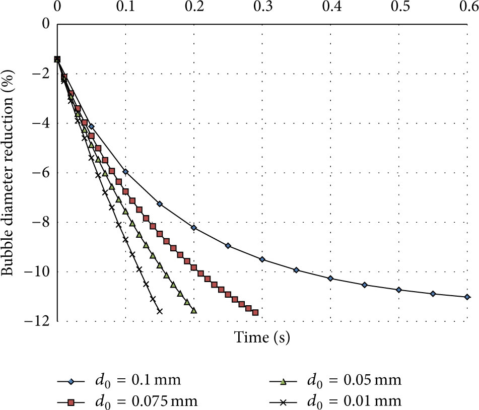
Bubble diameter percentage reduction versus time.
Bubble motion has been evaluated varying its relative velocity with respect to the water one. After a rapid transient phase, bubble motion depends only on water flow regardless of its starting velocity. In particular for the smallest bubble (d = 0.01 mm) the gap between bubble and water velocities is lower than in the other cases, according to previous consideration about bubble motion.
The water flow rate influence upon bubble motion has been investigated too, varying rotational speed. Results are reported in Figures 10 and 11, for the following cases:
Q = 7800 L/h; ω = 120 rad/s,
Q = 10000 L/h; ω = 125 rad/s,
Q = 13000 L/h; ω = 130 rad/s.

Polar coordinates of bubble trajectories for different water flow rates (d0 = 0.1 mm).

Percentage change of bubble diameter for different water flow rates (d0 = 0.1 mm).
Graphs show as the higher the flow rate, the higher the bubble penetration within the impeller duct and the diameter range of bubbles overstepping the duct becomes larger; in other words also larger bubbles can cross the duct.
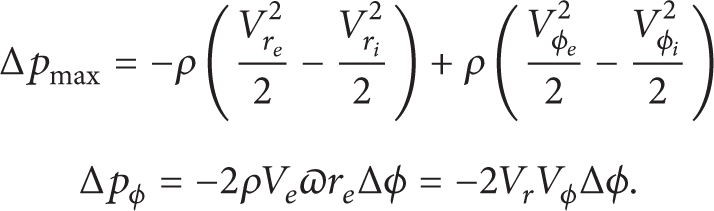
Numerical results about coalescence show that if the volume of the air bubble is smaller than the impeller volume, the two phases are stratified and an interface surface exists. The gas phase is included between the liquid phase before and above.
Water pushes the gas phase and the pressure inside the bubble increases. The interface surface moving itself toward the outlet of the impeller increases the pressure inside the gas phase.
In this way it is possible to plot the line of separation between the gas and the liquid phases.
In fact this interface is characterized by the same pressure value:
Fixing ϕ and computing r value which sets to zero the terms of equation, the points of the interface surface between the two phases inside the impeller can be evaluated, as showed in Figure 9.
6. Experimental Results
Three different situations have been analyzed:
formation of one bubble with volume less then pump volume,
formation of a lot of bubble in large time,
formation of bubble in short time.
In the first case, that is, when bubble volume is smaller than pump volume, the bubble behavior has been evaluated and described above. Theoretically we can describe the phenomenon applying the equations for each phase neglecting the slip conditions on the interface gas-liquid.
In this case the air phase is included between two liquid phases, in the outlet section and in the inlet section. In this way the behavior of the pump is intermittent because, in the first step, the liquid phase in the outlet region goes to the upper duct. The pump has to transfer the torque to a fluid with density smaller than the first one.
In the second case an important correlation between the frequency of the bubble generation and the capacity of the pump to move the two-phase flow exists. If the pump moves the gas flow faster than the incoming bubble near the inlet section, the pump will function in intermittent condition.
If the bubble formation is faster than the capacity of the pump to move the gas phase, near the inlet section, because of coalescence, bubbles with a volume greater than the pump volume can form. In this way the pump does not work and the gas phase will remain inside the impeller.
In real conditions these three behaviors will be present and the pump will function in irregular intermittent condition until the bubble volume is smaller than the impeller volume.
During the phase 1 the pump works with a periodic two-phase flow. The presence of a large bubble inside the impeller reduces the water flow rate. The air volume in this phase is still less than the volume of the impeller. In this way the pump can push away the air bubble.
If the bubbles volume increases for some reasons (different injection pressure, coalescence phenomenon) and the volume of the bubble is larger than the impeller volume, the pump work only with air and the water flow rate goes down to zero.
At this point, the reflux phenomenon starts, due to the presence of the water body force. The frequency around the zero value of the water flow rate increases until it goes down steady to zero value.
This is phase 3: only air flows inside the impeller and the water flow rate is zero all the time.
Particles that start from the low-pressure blade, or near this region, collide with the blade, slide on its surface, and go to the upper zone in the outlet zone of the rotor. The particles that crowd this region will change the blade profile and also the components of the velocity. Furthermore, experimental analysis showed that air bubbles move inside the inlet duct on the upper side of the blade and crowd near the inlet flange. This is a very important wake point. In fact, if the air flow rate is relatively high in this region the bubbles can coalesce and form bubbles that the impeller is not able to break into smaller sizes. It is well documented that bubbles with diameter in the range [0.1–0.2] mm pass easily from the inlet region to the outlet region following, with a good approximation, the water stream lines inside the impeller.
Bubbles with 0.3 < d < 0.5 mm can detach from the coalescence region and move inside the blade to the blade duct from the high pressure region to low pressure region until the impact with the blade. These bubbles inside the impeller are governed by the balance of the pressure gradient, momentum, and drag force and can find the equilibrium point inside the impeller. Growing the range of diameter of the bubbles 0.6 < d < 0.8–1 mm, the equilibrium point moves to the eye of the pump and the bubbles can coalesce with the bubbles near the inlet flange.
These conditions can also cause the total block of the water flow rate. By contour extraction software it is possible to evaluate the extension of the gas phase with respect to rotor vane, as reported in Figure 12. The cited sequence, from (a) to (f), has been acquired at 1 kHz and so the behavior of bubbles can be investigated duct by duct, from bubble motion to coalescence.

Coalescence images sequence.
In Figure 12(a), by contour analysis software, small bubbles starting from the inner radius, according to numerical results, move towards the blade side. In Figure 12(b) all bubbles coming from the rotor inlet, increasing radial coordinate, begin to coalesce, in small clusters. In Figures 12(c), 12(d), 12(e), and 12(f), coalescence goes on, generating a gas volume which keeps on invading the whole van. Energy transfer, due to Euler equation, is different between gas and liquid phases. If the coalescence phenomenon goes on, the percentage of gas will be more significant of the liquid phase and momentum variation transferred will be as small as liquid flow which rate decreases to zero. With such analysis a correlation between rotor angular speed, water flow rate, and gas phase extension can be carried out, identifying the limit working condition. In this work the correlation between gas phase extension and working limit condition has been highlighted, identified at 30% of gas phase in the rotor vane. In future works it will be better evaluated numerically.
7. Conclusion
The numerical model proposed allows evaluating the bubble motion and coalescence inside a centrifugal pump rotor. In particular bubble trajectories have been simulated achieving useful information about bubble diameter change and influence of initial velocities and water flow rate. The model better approximates bubbles behaviour when their presence is limited to a small volume fraction of the rotating duct, but it is in good agreement with experimental results achieved showing the trajectory of tracing particles (d < 0.4 mm) that go from blade base to the upper zone of impeller and to the next blade, due to pressure distribution. The model gives additional useful information about bubble coalescence and formation of gas zone within the rotor van, causing flow rate decrease and pulsation. Experimental results were in good agreement with numerical ones, both about bubble trajectories and about the formation of a coalescence zone which can be clearly distinguished by images sequences achieved by fast CCD camera and elaborated with specific routines for contour extraction. The contour extraction technique gives the most probable shape of the bubbles and the coalescence zone due to the definition of fuzzy approach. Moreover it can be used also to quantify the most probable bubble diameters, velocity of the coalescence phenomena, and all parameters useful to describe and evaluate this complex phenomenon.
The two-phase flow within centrifugal pumps has been becoming a fundamental issue also in geothermal plants, due to noncondensable gas dissolved in water to be extracted and thermally exploited, both for thermal and electrical power generation. The right understanding of condition leading to two-phase flow regime is a fundamental issue for the best operation of such plants, as in many other industrial applications as previously mentioned.
Footnotes
Nomenclature
Conflict of Interests
The authors declare that there is no conflict of interests regarding the publication of this paper.