Onboard Interference Prediction for the Cognitive Medium Access in the LEO Satellite Uplink Transmission

Abstract

Cognitive radio (CR) is an efficient way to increase spectrum efficiency for the small low earth orbit (LEO) satellite communication system. Due to the implementation difficulties, we focus on the CR in the uplink transmission. In CR, the cognitive medium access (CMA) is designed to enable the coexistence with the interferences from other systems. However, the CMA schemes designed for the terrestrial system cannot deal well with the global history of interferences in our system. Here, we design the memorized centroid bucket (MCB) scheme that can efficiently utilize the global history of interferences onboard without storing the complete interference samples. With MCB, we can achieve the effective long-term interference prediction to meet the special requirements of the LEO satellite. The key component in MCB is the matching algorithm that can help retrieve the useful historical information. In this paper, we propose three different matching algorithms and the corresponding MCB schemes. The schemes are also compared with the widely used Markovian method and the pair counting-based method. Among all the schemes, the Bayesian scheme MCB-FSNMI-Bayes is the best. The conclusion is validated experimentally with the real data that were collected by an LEO satellite.

1. Introduction

The low earth orbit (LEO) satellite systems, such as Iridium, have been used to provide the worldwide communication services for decades. The exclusive spectrum band over many countries is usually assigned to such systems. Recently, it is further suggested to use a small LEO satellite system to provide communications for the small-scale and short lived events [1]. Such a system usually consists of a few satellites that only cover a few regions at a time. Therefore, it is inefficient to assign the exclusive spectrum band for these systems as before. Cognitive radio (CR) [2] is an emerging technology that helps the communication system to utilize the spectrum more efficiently. It can help the small LEO satellite system find the available spectrum resource by avoiding the interferences [3].

However, CR for satellites is quite different from CR on the ground. One of the important reasons, as suggested in [3], is that CR is difficult to be implemented in satellite's downlink. It is because the satellite covers a lot of users that are remotely located. The available spectrum bands for the users could be quite different from each other due to the distinct local electromagnetic environments. So, we focus on the CR in the uplink transmission, in which the interferences can only be sensed and predicted by the satellite itself rather than the distributed terminals on the ground. The interferences are predicted in a centralized manner.

The channel characteristics of the satellite communication have been investigated for decades. The behavior of the land mobile satellite channel was characterized by a three-state Markov-chain-based model [4–7], which is well fit for the channel at the lower frequency band. For the higher frequency band, the tropospheric effect is also modeled in [8–11]. But the above models cannot be used to characterize the interference sensed by the satellite. The sensing result here is a combination of many remotely located users' signals that are transmitted on many different channels. In this paper, the sensing data are collected by the satellite at the lower bands where the local environment propagation is the main factor.

Cognitive medium access (CMA) is designed to enable the coexistence with the interferences from other systems. The method is usually designed to deal with the stochastic modeling and the prediction of the combination of different interferences. There is a CMA protocol that is proposed to model the medium access process as a constrained Markov decision process in [12]. The proposed protocol can provide a structured solution to utilize the spectrum in a proactive way. In the work, it is assumed that the interferences happen in an unslotted way. It is also assumed that the spectrum can be fully observed so that all the parallel channels can be observed simultaneously by energy detection. According to the solution, the channels are available as long as the collision rate is kept below some interference constraints. The effect of retransmission is further evaluated experimentally in [13]. There are also some other works that assume the partially observable CMA [14–17]. In this paper, the sensing data are collected by the satellite that can fully observe the spectrum, so the proposed onboard interference prediction scheme CMA is compared with the one in [12, 13].

In the works mentioned above, the receiver of CR is assumed to locate in some certain areas. Thus, the interference statics can be obtained based on the local history of interferences. Regarding the LEO satellite uplink transmission, however, the receiver is fast moving over different regions and the electromagnetic environment varies dramatically. So, an LEO satellite needs to utilize the global history of interferences rather than the local one.

The most straightforward way to utilize the global history of interferences is to build a database for different regions [18–20]. Building database is not feasible onboard for the LEO satellite, since an LEO satellite is always unable to store such huge data. Therefore, we could transmit the sensing results to the ground station and build a database there. However, this solution will bring great burden on the satellite downlink and lower the systematic reliability.

In this paper, we propose the memorized centroid bucket (MCB) schemes to achieve the long-term interference prediction by the suggested stationary spectral distribution (SSD) of interferences. The sensing results are reduced in frequency domain by clustering. Only the reduced information is stored by the system. Thus, the global history of interference can be utilized onboard, and the frequent spectrum handoff can be avoided as well. The most important module in these schemes is the matching algorithm that helps effectively retrieve the useful historical information for the prediction. There are three different MCB schemes with the different matching algorithms: MCB-ML that matches by the maximum likelihood criterion, MCB-FSNMI that matches with the proposed frequency sensitive normalized mutual information (FSNMI), and MCB-FSNMI-Bayes that matches by combining both the maximum likelihood method and the proposed prior information FSNMI. Besides the MCB schemes, the pair counting-based method and the Markovian method are also described. All these prediction schemes are evaluated and compared with the real data that were collected by an LEO satellite. It is validated that the Bayesian MCB scheme MCB-FSNMI-Bayes is the most proper scheme for the interference prediction here.

2. Problem Statement and System Description

The CMA in the LEO satellite uplink transmission is different from that on the ground because the electromagnetic environment of the satellite always keeps changing. As shown in Figure 1, for example, the LEO satellite moves around the earth for 5 times. Every time it passes the same latitude of the same hemisphere, the longitude has a small shift. It will take a very long time for the satellite to revisit the same place. Even if the satellite revisits the same place after a long time, the electromagnetic environment, however, may not be the same as before. So, the electromagnetic environment just keeps changing for an LEO satellite. Despite the fact mentioned above, the sensing results of the satellite may be similar in some cases. As shown in Figure 1, some of the interfering sources may be located at the overlapped covering area of the satellite antenna beams. The shadows in Figure 1 represent the covering areas of the satellite antenna beams. Therefore, the satellite may be interfered by the same interfering source while visiting the adjacent areas. And the interference samples collected by the satellite may be similar. This situation could happen when the satellite visits the adjacent areas in two adjacent passes as shown in Figure 1 or after a long time. However, it is difficult to utilize such similarities of the sensing results, because the similarities are hard to model without the prior knowledge about locations of the interfering sources. So, rather than using the widely used methods for CMA, we design a novel interference prediction scheme for the LEO satellite to utilize the global history effectively and efficiently. This scheme can be implemented with the onboard computational and storing capabilities of the satellite.

Figure 1

Changes of the electromagnetic environment in the LEO satellite uplink.

There is a special problem in designing the CMA in the LEO satellite uplink transmission: the overhead of the frequent spectrum handoffs is very expensive here. The connection between a small LEO satellite constellation and a terminal is very precious, because a small LEO satellite system can only support the transmission for a few times in a day. The uplink transmission cannot afford to be interrupted by the frequent spectrum handoffs. We prefer to predict the interference in the long run in order to avoid the frequent spectrum handoffs. Therefore, the observation time should firstly be segmented into a series of periods before the prediction. Then, the frequencies to be interfered could be predicted at the beginning of each period.

In our system, we firstly segment the observation time. After the proper segmentation, we can obtain some insight about the practical electromagnetic environment by observing the real data that were collected by an LEO satellite. Some of the real data are shown in Figure 2 for the illustration. In Figure 2, the values on the X-axis represent the time at which the interferences were sampled, and the values on the Y-axis represent the frequencies of the interferences. We think that some interference occurs at a specific time and frequency if the measured power level is higher than a given threshold. The dot points in Figure 2 represent the existences of the interferences in the 2-dimensional space. There are two subfigures in Figure 2, which represent the interference samples that were collected at different time. The samples shown in Figure 2(a) and those shown in Figure 2(b) are separated in time for about 7 days.

Figure 2

Stationary spectral distribution.

Firstly, it could be seen that both the samples in Figures 2(a) and 2(b) can be properly segmented into two periods. After the segmentation, the interferences in the first and in the second period of Figure 2(a) can be partitioned in frequency domain with two sets of rectangles that are called “spectrum partition 1” and “spectrum partition 2,” respectively. It can be inferred from the rectangles that we can partition in frequency domain the samples collected early and the samples collected later similarly for each well-segmented period. This phenomenon is named as the stationary spectral distribution (SSD) of interferences here. Moreover, it can be seen that the interference samples in Figure 2(b) are distributed similarly to those in Figure 2(a) in frequency domain. At the same time, the two spectrum partitions in Figure 2(b) are identical to those in Figure 2(a). This illustrates the similarities of the sensing results as mentioned above. It also shows the possibility of using the spectrum partition to find the similar interference samples.

SSD is reasonable if we think over the practical situations. In practice, the frequently occupied spectrum bands are dependent on the regions that the LEO satellite flies over. In a properly segmented period, all the sensing results might be collected over the same region. So, in such a period, the early observed interferences could be highly correlated with the later ones in frequency domain. Then, it is possible to represent the samples in a period with their spectrum partition by SSD. When there are two spectrum partitions similar to each other, the satellite may encounter the similar interferences.

By SSD, we can design a scheme to predict for each period the spectrum partition of the remaining samples with the spectrum partition of a few samples collected at the beginning. The spectrum partition of the coming interferences can be well predicted without observing all the samples. Furthermore, it is possible for us to find a similar spectrum partition by utilizing the historical information. Such a similar spectrum partition of the same samples can imply a similar spectral distribution of the interference samples. Therefore, the prediction and the similarity of the spectrum partitions can be combined to predict the frequencies that will be interfered in the long run.

Before the detailed description of the prediction method, we have several definitions to characterize the memorization of this history-based system. Firstly, we define in this paper the memorized period as the information of a period memorized by the system. The information contained in the memorized period depends on the prediction scheme we use. The memorized period stored by the prediction scheme above contains the reduced information, which consists of the memorized spectrum partition information (MSPI) and the frequencies that were interfered (FWI). MSPI is defined as the historical information that can guide the partition of the collected samples. It is extracted from the spectrum partition of the interference samples in the previous period. FWI is defined as the set of frequencies that have been interfered in the previous period. It can be obtained directly from the interference samples. However, the memorized period stored by some other schemes may need to contain the full dataset of the interferences. We also define the memory depth as the number of the memorized periods stored by the satellite onboard. The size of the memory depth is usually constrained by the onboard storing capability. More than one similar memorized period may be retrieved for the prediction. Then, we define the packet size as the number of the memorized periods that are retrieved. The true partition is defined as the most reasonable spectrum partition of the samples. Meanwhile, the memorized partition is defined as the partition of the samples with the memorized period. We can partition the samples in the normal way for the true partition and partition them with the MSPI of a memorized period to obtain the memorized partition.

So, the prediction procedure can be described in detail with the block diagram in Figure 3. For instance, we want to predict the frequencies that will be interfered for the first period in Figure 2(b). Firstly, we collect a few samples at the beginning of the period. After the collection, we can predict the spectrum partitions of the remaining samples in the period by SSD. The prediction of the spectrum partition is the true partition here. Then, we utilize the memorized periods to obtain the memorized partitions and try to find the memorized partitions that are most similar to the true partition. According to Figure 2, we can examine the first period in Figure 2(a). In Figure 2, the “spectrum partition 1” can be regarded as the MSPI of this period. Moreover, since the samples in the first period in Figures 2(b) and 2(a) have the same spectrum partition, the memorized partition mentioned above will be similar to the true partition. Then, the FWI of the first period in Figure 2(a) can be retrieved for prediction. Because the similar spectrum partitions may represent the similar spectral distributions of the interference samples, we can predict that the frequencies in the retrieved FWI may also be interfered in the remaining time of the first period in Figure 2(b). This method can achieve the long-term prediction of interference and help us save the onboard computational and storing resources.

Figure 3

Prediction procedure.

We have described the long-term onboard prediction procedure that is inspired by the observation of the real interference samples. However, the generation, the storing, and the comparison of the spectrum partitions need to be further refined for the implementation. Here, we propose the onboard interference prediction scheme memorized centroid bucket (MCB) whose system model is shown in Figure 4. In this model, the spectrum can be fully observed by the full spectrum sensing, and we predict the interferences for the current period. Firstly, a few samples are collected by the initial scan at the beginning of the current period. At the same time, the interference samples in the last period are clustered in frequency domain so as to obtain a set of centroids that represent the mean frequencies of the different clusters of samples. With the set of centroids, the interference samples can be partitioned in frequency domain by the nearest centroid rule. The set of centroids can represent the MSPI of the last period. Thus, the memorized period that consists of the MSPI and the FWI of the last period is stored in the centroid bucket. The centroid bucket is the component that stores the memorized periods. Then, we need to compare the spectrum partitions and retrieve the similar memorized periods. There is a matching algorithm in the system that matches the samples collected in the initial scan to the most similar memorized periods. There are three different kinds of MCB schemes with the different matching algorithms.

Figure 4

System model of the memorized centroid bucket scheme.

The matching can be achieved in a direct way with the memorized periods and the data collected in the initial scan. We calculate the likelihood of the collected samples given the different MSPI. By the maximum likelihood criterion, the memorized periods, whose MSPI will lead to the maximal likelihood, are matched, and their FWI are retrieved for the prediction (MCB-ML). Furthermore, we can match the samples collected in the initial scan more efficiently by comparing the true partition and the memorized partitions of them. These two kinds of partitions of the collected samples will be described in Section 3.2. The result of the comparison is the proposed prior information FSNMI. FSNMI can be used alone to match the samples and predict the interferences (MCB-FSNMI). We can also combine FSNMI with the maximum likelihood method to match the samples in a Bayesian way (MCB-FSNMI-Bayes). The prior information FSNMI can complement the maximum likelihood method by utilizing the samples in the initial scan as a whole. By comparing the three MCB schemes with the prediction procedure shown in Figure 3, it can be shown that MCB-FSNMI-Bayes is the full implementation of the procedure, while the other two schemes are the simplified ones.

3. Matching and Prediction Algorithms

We have described SSD, the prediction procedure, and the system model of the MCB schemes as above. However, the feasibility and the performances of the MCB schemes are highly related to the matching algorithms that can help retrieve the useful historical information. The difficulty in designing such a matching algorithm lies in the efficient utilization of the small amount of data that are collected in the initial scan. After matching, we will predict the frequencies to be interfered in the remaining time of the current period.

In this section, we propose the different matching algorithms of the MCB schemes, and the pair counting-based method as well. Then, the prediction strategy based on the retrieved historical information is introduced, and the Markovian predictor is also analyzed. It will be shown that the Markovian method is suboptimal to the problem.

The memory depth and the packet size are represented with L and M, respectively. It is assumed that the current period is the sth period in sequence. In Figure 2, the interference samples are plotted in a 2-dimensional space of time and frequency. However, after the proper time segmentation, the samples X and Y discussed in the following sections are the frequencies of the interferences.

3.1. Matching by Pair Counting

Before introducing the matching algorithms for the information retrieval in the MCB schemes, we firstly discuss a more direct yet inefficient method: the pair counting-based method. The interference samples in two periods are compared by counting the number of the occurrences of interference at different frequencies. The interference samples in two periods are regarded as similar to each other if the interference often occurs at the same frequencies. The similarity can be calculated in a similar way as introduced in [21]. Suppose that the interference occurs at the frequency $f_k$ for $N_{ik}$ times in the ith period and $N_{jk}$ in the jth period. As shown in (1), the similarity between the interference samples in the ith and the jth period can be computed with the counts of the common elements $\{\min (N_{ik},N_{jk})\}$ . Thus, the memorized periods with the highest similarities will be matched. Consider the following:

$$\begin{array}{cc}& \text{Sim}\left(i,j\right)=\frac{{\left[{\sum }_k\min \left(N_{ik},N_{jk}\right)\right]}^2}{\left[{\sum }_k{N}_{ik}{\sum }_k{N}_{jk}\right]}.\end{array}$$

(1)

The pair counting-based matching algorithm is designed based on (1) as in Algorithm 1.

Algorithm 1: The matching algorithm of the pair counting-based method.

Require:

       $Y_i$ : all the interference samples in the ith period.

       $f_i$ : the FWI of the ith period.

       $X_s$ : the samples collected in the initial scan of the sth period.

Ensure:

      for   $s=1$ to ∞  do

           for   $i=s-L$ to $s-1$   do

                  Calculate Sim(s, i) between $X_s$ and $Y_i$ by (1).

                  Store Sim(s, i) in $D_s$ .

           end for

           Find the  largest  M values in $D_s$ and the corresponding sequence number.

           Find the FWI with the same sequence number. (Matching)

      end for

This method does not need to be implemented in the same way as the MCB. However, the memorized periods of the scheme need to contain all the interference samples and the corresponding FWI in the previous L periods. This is inefficient and unrealistic considering the storing capability of an LEO satellite. Moreover, it is not an effective method for us to compare the initial scan with a memorized period, since the data collected in an initial scan is usually too small to use here and the complete dataset contains the disturbing noise. This conclusion is validated by the experiments on the real data. So, we need to design some other matching algorithms further.

3.2. Spectrum Partition

The MCB schemes are based on the spectrum partitions of the interference samples in frequency domain. We reduce the interference samples in a period to their MSPI in MCB. Here, the partitioning is carried out by clustering the samples with the most well-known centroid algorithm K-means [22]. This algorithm is used to implement the “clustering for the MSPI” and the “clustering” block in Figure 4. The input of the block is the spectral information of all the interference samples, and the output is the centroid set that represents the mean frequencies of the different clusters of interference samples.

K-means is an iterative algorithm that will converge after iterating for enough times. It should be noticed that the final results are dependent on the initial centroids to a great extent. So, we assume that the initial centroids are the same for all the periods to make the partitions consistent. And, it is reasonable to place the initial centroids evenly in frequency domain. Let the number of the initial centroids be N. For the example of the ith period, the kth initial centroid should be placed at the frequency $c_{ik}^{(0)}$ . So, we have

$$\begin{array}{cc}& c_{ik}^{\left(0\right)}-c_{i\left(k+1\right)}^{\left(0\right)}=\text{const}.,\hspace{1em}1\le k\le N-1.\end{array}$$

(2)

After t iterations, the centroid will be moved to $c_{ik}^{(t)}$ . When the algorithm converges, the number of the centroids in the ith period will be reduced to $L_i$ . The final centroids $\{c_{ik}\}$ are contained in the set $C_i$ .

Some of the centroids may vanish as the algorithm iterates. However, we still keep the initial indexes $\{k\}$ of the remaining centroids to compute FSNMI in Section 3.4, which contain the spectral positional information of the centroids.

The samples collected in the initial scan can be partitioned in frequency domain by K-means for the true partition. In a true partition, the samples belong to the different clusters in frequency domain, and thus they are well partitioned. On the other hand, the samples can also be partitioned in frequency with the MSPI for the memorized partition. With the set of centroids that represent the MSPI, the spectrum can be partitioned by the nearest centroid rule. By the nearest centroid rule, a given sample is attributed to the cluster whose centroid is nearest to it in frequency domain. Therefore, the interference samples are partitioned with a given set of centroids in frequency domain. Clustering is not new to spectrum sensing [23, 24] where it is often used to divide the groups of nodes in the cognitive radio networks. But it is now used to partition spectrum for the data reduction and information retrieval.

3.3. Matching Algorithms in MCB

The samples in the initial scan are matched to the memorized periods properly in MCB in order to retrieve the historical information. In fact, MCB could match by SSD not only the initial scan but also the rest of the current period in a predictive way. With the MSPI, the ideal way to match is based on the posterior probability of the set of centroids given all the samples in the sth period. The sets of centroids that have the highest posterior probabilities are matched to the sth period. Although by the initial scan we only collect a few samples instead of all the samples in the period, we can approximate the posterior probability by SSD. The matching algorithm based on the posterior probability is a Bayesian algorithm. Here, we derive the basic formula of this Bayesian matching algorithm and design a simplified version of the algorithm by the maximum likelihood criterion. The Bayesian algorithm will be described in Section 3.4.

We utilize here not only the w frequency samples $X=\{x_1,x_2,\dots ,x_w\}$ collected in the initial scan but also the unknown samples R in the remaining time of the period. According to SSD, we can partition X and R in the similar way for the sth period, which implies some strong correlation between them. Therefore, it is reasonable to assume that the distribution of R can be inferred from that of X. Thus, the posterior probability can be approximated under this reasonable assumption. Let $M=1$ and $L=\infty$ , and $1\le i\le s-1$ . The sequence number of the matched memorized period is represented by $Idx$ (s). The set of centroids that has the largest posterior probability given X and R can be found by the following equation:

$$\begin{array}{l}Idx\left(s\right)=\underset{1\le i\le s-1}{\text{argmax}\hspace{0.17em}}P\left(C_i\hspace{0.17em}|\hspace{0.17em}X,R;s\right)\\ =\underset{1\le i\le s-1}{\text{argmax}\hspace{0.17em}}P(C_i,X,R;s)\\ =\underset{1\le i\le s-1}{\text{argmax}}\hspace{0.17em}P\left(R\hspace{0.17em}|\hspace{0.17em}X,C_i;s\right)P\left(X\hspace{0.17em}|\hspace{0.17em}{C}_i;s\right)P\left(C_i;s\right).\end{array}$$

(3)

The distribution of R can be inferred from that of X, though the data in R are unknown to us. It can be further assumed that the data in R are almost certain if X is already known. Thus, we can approximate $P(R\hspace{0.17em}|\hspace{0.17em}X,C_i;s)$ in (3) to be 1. And, the formula is approximated as follows:

$$\begin{array}{cc}& Idx\left(s\right)\approx \underset{1\le i\le s-1}{\text{argmax}}\hspace{0.17em}P\left(X\hspace{0.17em}|\hspace{0.17em}{C}_i;s\right)P\left(C_i;s\right).\end{array}$$

(4)

The prior probability $P(C_i;s)$ cannot be acquired immediately since the similarity between the sensing results is hard to model in our problem. Therefore, a simple solution is to treat the different sets of centroids equivalently. In this case, the initial scan is matched by the maximum likelihood criterion (MCB-ML) in which $P(C_i;s)$ equals $1/(s-1)$ .

According to K-means, the elements of each cluster are assumed to scatter around their centroid by Gaussian distribution, and the variances of the different clusters in each period are the same. The variance ${\sigma }_i^2$ can be estimated in the normal way. The samples collected in the initial scan can be treated independently in time. Therefore, it can be derived from (4) that

$$\begin{array}{l}Idx\left(s\right)\approx \underset{1\le i\le s-1}{\arg \hspace{0.17em}\max }\left(P\left(X\hspace{0.17em}|\hspace{0.17em}{C}_i;s\right)\right)\\ =\underset{1\le i\le s-1}{\text{argmax}}\left(\ln \left({\displaystyle \prod }_{q=1}^{w}P\left(x_q\hspace{0.17em}|\hspace{0.17em}{C}_i;s\right)\right)\right)\\ =\underset{1\le i\le s-1}{\text{argmax}}{\displaystyle \sum }_{q=1}^w\ln \left(\frac{1}{\sqrt{2\pi }{\sigma }_i}\exp \left(-\frac{{\left(x_q-c_{iq}^{*}\right)}^2}{2{{\sigma }_i}^2}\right)\right)\\ =\underset{1\le i\le s-1}{\text{argmax}}\left(-w\ln \left(\sqrt{2\pi }{\sigma }_i\right)-{\displaystyle \sum }_{q=1}^w\frac{{\left(x_q-c_{iq}^{*}\right)}^2}{2{{\sigma }_i}^2}\right),\\ \phantom{fffffffffffccccccfffsfffff}{c}_{iq}^{*}=\underset{c_{ik}\in C_i}{\text{argmin}}\left(\left|x_q-c_{ik}\right|\right).\end{array}$$

(5)

Then, we can define the distance ${\delta }_{i,s}$ according to (5) to measure the spectral difference between the interference samples in the ith period and the sth period. A smaller distance ${\delta }_{i,s}$ can represent a higher similarity between them. Here, this distance can be calculated by the following equation:.

$$\begin{array}{cc}& {\delta }_{i,s}=w\ln \left(\sqrt{2\pi }{\sigma }_i\right)+{\displaystyle \sum }_{q=1}^w\frac{{{(x}_q-c_{iq}^{*})}^2}{2{{\sigma }_i}^2},\\ \phantom{vvvvvvvvvvvv}{c}_{iq}^{*}=\underset{c_{ik}\in C_i}{\arg \hspace{0.17em}\min }\left(\left|x_q-c_{ik}\right|\right).\end{array}$$

(6)

The matching algorithm of MCB-ML is designed based on (6) as in Algorithm 2.

Algorithm 2: The matching algorithm of MCB-ML.

Require:

      $C_i$ : the set of centroids (MSPI) of the ith period.

      $f_i$ : the FWI of the ith period.

      $X_s$ : the samples collected in the initial scan of the sth period.

Ensure:

     for   $s=1$ to ∞  do

           for   $i=s-L$ to $s-1$   do

                 for   $q=1$ to w  do

                       Find the centroid $c_{iq}^{*}$ in $C_i$ that is closest to $x_q$ .

                 end  for

                 Calculate ${\delta }_{i,s}$ between $C_i$ and $X_s$ by (6).

                 Store ${\delta }_{i,s}$ in $D_s$ .

           end  for

           Find the  smallest  M values in $D_s$ and the corresponding sequence number.

           Find the FWI with the same sequence number. (Matching)

     end  for

For this maximum likelihood algorithm, the number of the samples collected in the initial scan is usually too small, and each of the samples is treated individually. Furthermore, a Bayesian algorithm is more suitable to deal with such small data. The performance will be improved if we obtain a reasonable prior $P(C_i;s)$ for each memorized period rather than treat them equivalently. And more useful information will be extracted from the initial scan if we can treat these collected samples as a whole. Therefore, it is helpful if we can extract some useful prior information by utilizing the small data altogether.

3.4. Frequency Sensitive Normalized Mutual Information

We only have the incomplete information in the matching process of MCB. This incomplete information consists of the MSPI, the FWI, and a few samples collected in the initial scan of the current period. This information is not sufficient for many statistical methods. However, by SSD, some extra information can be obtained by computing the similarities between the true partition and the memorized partitions of the same samples collected in the initial scan. This information is the frequency sensitive normalized mutual information (FSNMI).

Besides the partitions and the likelihood that we calculate in Section 3.3, we also take into account the initial indexes $\{k\}$ that contain the spectral positional information of the centroids. As mentioned in Section 3.2, these indexes are preserved before the K-means algorithm begins to iterate. With all these information, we can obtain the FSNMI between different partitions. This information can be approximated as the prior information in (4).

We utilize the samples collected in the initial scan as a whole by extracting the spectral partition information of them. By clustering, we can obtain the true partition of these samples. According to SSD, the true partition of the samples contains the correlated information between the collected data X and unknown data R. So, the samples collected in the initial scan are treated altogether by clustering. Therefore, it is possible to learn the prior information $P(C_i;s)$ by comparing the true partition with the memorized partitions. Although this comparison is not prior to X, it is still prior to the major part of the current period, the data R. So, the result of this comparison can be used to approximate the prior information. We represent this result with FSNMI. FSNMI can be used alone to match the data (MCB-FSNMI), and it can also be combined with the maximum likelihood method (MCB-FSNMI-Bayes).

It is assumed that the true partition of X in the sth period consists of the nonoverlap subsets (clusters) ${\mathbf{V}}^s$ . Meanwhile, the memorized partition of X by the MSPI in the ith period is the nonoverlap subsets (clusters) ${\mathbf{U}}_i^s$ . These two partitions of the samples in the initial scan are shown in Table 1. For example, as shown in Table 1, there are $n_{12}$ samples in the cluster $V_2$ and the cluster $U_1$ at the same time. Also, there are totally $a_1$ samples in the cluster $U_1$ and $b_2$ samples in the cluster $V_2$ .

Table 1

Table of the two partitions.

${\mathit{U}}_i^s$ ∖ ${\mathit{V}}^s$	$V_1$	$V_2$	…	$V_{C(s)}$	Sums
$U_1$	$n_{11}$	$n_{12}$	…	$n_{1C}$	$a_1$
$U_2$	$n_{21}$	$n_{22}$	…	$n_{2C}$	$a_2$
…	…	…	…	…	…
$U_{R(i,s)}$	$n_{R1}$	$n_{R2}$	…	$n_{RC}$	$a_R$
Sums	$b_1$	$b_2$	…	$b_C$	w

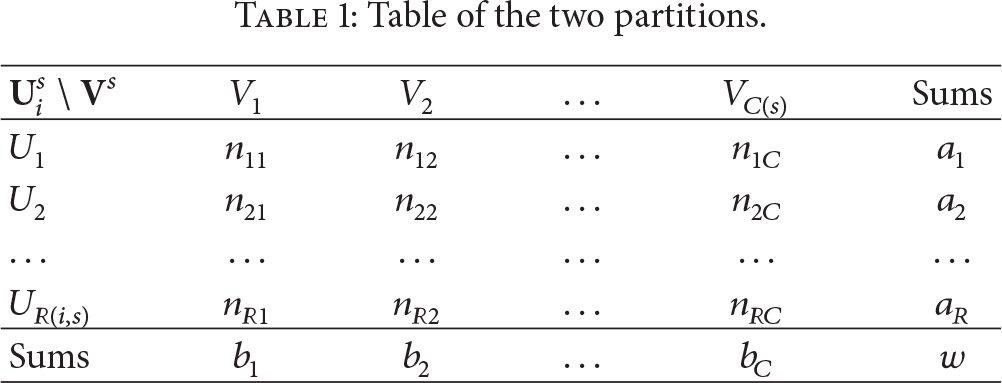
The similarity between two partitions of the same samples can be quantified by computing the normalized mutual information (NMI) between them [21]. Let 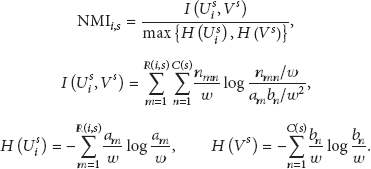$M=1$ and $L=\infty$ , and $1\le i\le s-1$ . With the notations shown in Table 1, NMI can be calculated by the following equation:

$$\begin{array}{cc}& \text{NM}{\text{I}}_{i,s}=\frac{I\left(U_i^s,V^s\right)}{\max \left\{H\left(U_i^s\right),H\left(V^s\right)\right\}},\\ I\left(U_i^s,V^s\right)={\displaystyle \sum }_{m=1}^{R\left(i,s\right)}\hspace{0.17em}{\displaystyle \sum }_{n=1}^{C\left(s\right)}\frac{n_{mn}}{w}\log \frac{n_{mn}/w}{a_m{b}_n/w^2},\\ H\left(U_i^s\right)=-{\displaystyle \sum }_{m=1}^{R\left(i,s\right)}\frac{a_m}{w}\log \frac{a_m}{w},\hspace{1em}\hspace{1em}H\left(V^s\right)=-{\displaystyle \sum }_{n=1}^{C\left(s\right)}\frac{b_n}{w}\log \frac{b_n}{w}.\end{array}$$

(7)

However, NMI is not sufficient to represent the similarity between the spectrum partitions. It is only related to the partitions of the samples, and it cannot represent the positions of the interferences in frequency domain. So, the prior information is further learnt by adding some frequency sensitive information to NMI. It is useful to utilize the relationship that the less difference of the spectral positions between two sets of centroids implies the more similarity between them. The precise frequencies of the centroids are not used as the frequency sensitive information. Rather, we represent the information with the initial indexes $\{k\}$ of the centroids. It is because this method can bring more regularization for the matching algorithm. Otherwise, the precise frequencies may cause overfitting of the algorithm due to the small number of the input data X. In the memorized partition ${\mathbf{U}}_i^s$ , the initial indexes of the centroids that the samples belong to are represented by the vector ${\mathbf{I}}_i^s$ . In the true partition ${\mathbf{V}}^s$ _, the indexes are represented by the vector ${\mathbf{I}}^s$ . Therefore, FSNMI can be computed as follows:

$$\begin{array}{cc}& \text{FSNM}{\text{I}}_{i,s}=\text{NM}{\text{I}}_{i,s}\times (1-\frac{\parallel I_i^s-I^s\parallel }{{\rho }_s}),\\ \phantom{dddddddddddddd}{\rho }_s=\underset{1\le j\le s-1}{\max }\parallel I_j^s-I^s\parallel .\end{array}$$

(8)

Thus, the memorized periods are matched in MCB-FSNMI by (7) and (8). The algorithm is designed as in Algorithm 3.

Algorithm 3: The matching algorithm of MCB-FSNMI.

Require:

      $C_i$ : the set of centroids (MSPI) of the ith period.

      $f_i$ : the FWI of the ith period.

      $X_s$ : the samples collected in the initial scan of the sth period.

Ensure:

      for   $s=1$ to ∞ do

            Cluster $X_s$ for ${\mathit{V}}^s$ and ${\mathit{I}}^s$ .

            for   $i=s-L$ to $s-1$   do

                  Partition $X_s$ with $C_i$ for ${\mathit{U}}_i^s$ and ${\mathit{I}}_i^s$ .

                  Calculate ${\text{FSNMI}}_{i,s}$ by (7) and (8).

                  Store ${\text{FSNMI}}_{i,s}$ in $D_s$ .

            end for

            Find the largest  M values in $D_s$ and the corresponding sequence number.

            Find the FWI with the same sequence number. (Matching)

      end for

Furthermore, the Bayesian method MCB-FSNMI-Bayes can be obtained if we combine MCB-ML with the learnt prior information FSNMI. Then the formula in the matching algorithm can be derived from (4) and (5) as follows:

$$\begin{array}{l}Idx\left(s\right)=\underset{1\le i\le s-1}{\text{argmax}}\left(\ln P\left(X\hspace{0.17em}|\hspace{0.17em}{C}_i;s\right)+\ln P\left(C_i;s\right)\right)\\ =\underset{1\le i\le s-1}{\text{argmax}}(\phantom{{\displaystyle \sum }_{q=1}^w\frac{{\left(x_q-{c^{*}}_{iq}\right)}^2}{2{{\sigma }_i}^2}}-w\ln \left(\sqrt{2\pi }{\sigma }_i\right)\\ \phantom{\text{cccccccccc}}\phantom{FF}-{\displaystyle \sum }_{q=1}^w\frac{{\left(x_q-c_{iq}^{*}\right)}^2}{2{{\sigma }_i}^2}+\ln \text{FSNM}{\text{I}}_{i,s}).\end{array}$$

(9)

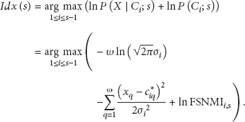
According to (9), the distance ${\delta }_{i,s}$ can be calculated by the following equation, which is an extension of the distance in MCB-ML:

$$\begin{array}{cc}& {\delta }_{i,s}=w\ln \left(\sqrt{2\pi }{\sigma }_i\right)+{\displaystyle \sum }_{q=1}^w\frac{{\left(x_q-c_{iq}^{*}\right)}^2}{2{{\sigma }_i}^2}-\ln \text{FSNM}{\text{I}}_{i,s},\\ \phantom{ssssssssssssssssssssssssss}{c}_{iq}^{*}=\underset{c_{ik}\in C_i}{\arg \hspace{0.17em}\min }\left(\left|x_q-c_{ik}\right|\right).\end{array}$$

(10)

The matching algorithm of MCB-FSNMI-Bayes is designed based on (10) as in Algorithm 4.

Algorithm 4: The matching algorithm of MCB-FSNMI-Bayes.

Require:

      $C_i$ : the set of centroids (MSPI) of the ith period.

      $f_i$ : the FWI of the ith period.

      $X_s$ : the samples collected in the initial scan of the sth period.

Ensure:

    for   $s=1$ to ∞ do

           Cluster $X_s$ for ${\mathit{V}}^s$ and ${\mathit{I}}^s$ .

           for   $i=s-L$ to $s-1$   do

                 Partition $X_s$ with $C_i$ for ${\mathit{U}}_i^s$ and ${\mathit{I}}_i^s$ .

                 Calculate ${\text{FSNMI}}_{i,s}$   by (7) and (8).

                 for   $q=1$ to w  do

                       Find the centroid $c_{iq}^{*}$ in $C_i$ that is closest to $x_q$ .

                 end for

                 Calculate ${\delta }_{i,s}$ between $C_i$ and $X_s$ by (10).

                 Store ${\delta }_{i,s}$ in $D_s$ .

           end for

           Find the smallest  M values in $D_s$ and the corresponding sequence number.

           Find the FWI with the same sequence number. (Matching)

     end for

3.5. Prediction and Evaluation

After the matching process, we can make the long-term predictions with the matched results, which predict the frequencies to be interfered in the remaining time of the current period. The frequencies that are predicted to be idle may be used by the system in the remaining time of the current period. The length of the initial scan is very short in time, and the remaining time is often several tens of times longer. This proactive CMA enables the long-term occupation of the same channel. It is very important to the transmission of an LEO satellite, because the overhead of the spectrum handoff for the CMA in the LEO satellite uplink is much more expensive than that for the terrestrial CMA system. The spectrum handoff during a period happens when the long-term prediction fails, which is, however, not the topic of this study. Our focus here lies on the long-term interference prediction whose performance determines the feasibility of the CMA in our system. The performance is evaluated by the $F_p$ -score, the probability of detection ( $P_d$ ), and the spectrum loss rate (SLR).

The MCB schemes and the pair counting-based method have the same strategy to predict with the matched results. The matched results are the FWI of the M retrieved memorized periods. It is reasonable to predict that the same frequencies are to be interfered again for the rest of the current period. A larger packet size will lead to a higher $P_d$ in predicting the frequencies to be interfered. It means that the communication is less likely to be interrupted by the interference, if the satellite occupies the channels according to the prediction. However, a larger packet size will also bring more false alarm of the interference, by which the spectrum resource may be wasted. So there is a tradeoff while choosing the packet size. The FWI of different memorized periods are merged by OR rule. In our system, the FWI of the jth matched memorized period are represented by the frequency set $F_{s,j}$ . And the resulting frequencies in the set $F_s$ are predicted to be interfered for the sth period. Consider the following:

$$\begin{array}{cc}& F_s=F_{s,1}\parallel F_{s,2}\parallel \cdots \parallel F_{s,M}.\end{array}$$

(11)

There may be some loss in performance when using OR rule to merge the information of the different memorized periods. The different matched memorized periods are treated equivalently if OR rule is used. A more sophisticated strategy, for example, a weighting strategy could be utilized to merge the information, which may improve the performance. Such a strategy should be designed carefully, and it needs to be further investigated.

The MCB schemes and the pair counting-based method should also be compared with the widely used Markovian method. It is assumed in [12, 13] that the system can fully observe the spectrum, which is the same as our system. We can model the occurrences of interferences in each period as a Markov chain reasonably for our problem. The channels are regarded to be available as long as the collision rate is kept below some interference constraints. The experimental test bed in [13] measures the throughput and collision rate experimentally. It also adjusts the transmission rate so that the interference constraint can be met. For example, a randomized policy is adopted to transmit in the idle channel with the lowest interference arrival rate, so that the interference level is lower than the cumulative interference constraint. Here the interference arrival rate represents the rate of the interference occurrences. We define this rate as λ and the transmission slot duration as T for a specific channel. In our system, T could represent the length of a well-segmented period. In [12], the expected immediate cost d for communicating in the channel can be computed as follows:

$$\begin{array}{cc}& d=1-e^{-\lambda T}.\end{array}$$

(12)

To achieve the long-term proactive CMA with the Markovian method above, we observe each channel for some time and evaluate it with the immediate cost d. In the prediction, all the channels are assumed as available beforehand, but they need to be evaluated by the immediate costs. The channels whose immediate costs exceed the predefined threshold are predicted to be interfered sometimes in the current period. It is not needed to use OR rule to merge the different matched results here. The Markovian prediction algorithm is designed as in Algorithm 5.

Algorithm 5: The prediction algorithm of the Markovian method.

Require:

      $Y_i$ : all the interference samples in the ith period.

      $X_s$ : the samples collected in the initial scan of the sth period.

Ensure:

     for   $s=1$ to ∞ do

            Collect all the samples in $X_s$ and $Y_{s-j}j=\mathrm{1,2},\dots ,L$ .

            Calculate λ for all the frequencies (channels) with the collected samples and T.

            Calculate d for all the frequencies (channels) with λ and T by (12).

            Find the frequencies (channels) that have a d greater than the predefined threshold.

            (These found frequencies (channels) will be interfered in the remaining time of the sth period.)

     end for

Compared with MCB, the Markovian method cannot utilize the global history efficiently. In the Markovian method, the parameters, such as the arrival rate, are usually assumed as constant. However, the interference arrival rate in our problem varies as the LEO satellite moves around the earth. Thus the Markovian method will treat the interferences of different regions equivalently. As the memory depth gets larger, MCB could retrieve some more similar memorized periods and perform better while the prediction of the Markovian method is suboptimal. 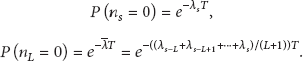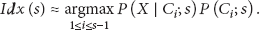Apart from the variables T and L defined above, ${\lambda }_i$ is defined as the rate of the interference occurrences in the ith period at a specific frequency (channel). The sth period is the current period. Let $n_s$ be the number of interference occurrences estimated by ${\lambda }_s$ and let $n_L$ be the number of interference occurrences estimated by ${\lambda }_{s-j}$ ( $j=\mathrm{0,1},\dots ,L$ ). Both $n_s$ and $n_L$ are the number of the interference occurrences estimated for a specific frequency (channel) in the sth period. Then we have the following equations according to the exponential distribution in a Markov chain:

$$\begin{array}{cc}& P\left(n_s=0\right)=e^{-{\lambda }_{s}T},\\ P\left(n_L=0\right)=e^{-\stackrel{-}{\lambda }T}=e^{-\left(\left({\lambda }_{s-L}+{\lambda }_{s-L+1}+\cdots +{\lambda }_s\right)/\left(L+1\right)\right)T}.\end{array}$$

(13)

The probabilities in (13) represent the probabilities that no interference is expected to happen by ${\lambda }_s$ and ${\lambda }_{s-j}$ ( $j=\mathrm{0,1},\dots ,L$ ), respectively. These two probabilities are identical only if L is 0, and they may vary widely for an LEO satellite. So, a memory depth that is larger than 1 is improper for the Markovian method. However, we cannot obtain the true rate ${\lambda }_s$ for the sth period with $X_s$ that is too small for the estimation. The rate ${\lambda }_s$ is estimated with the samples collected in both the initial scan of the sth period and the previous periods, and ${\lambda }_s$ is approximated with the mean rate of the different interference occurrences. Then, the Markovian method can only utilize the correlation between the current period and the recent memorized ones. Therefore, it is always suboptimal to our problem.

To evaluate the performance, we firstly compute $P_d$ that can tell us how many of the interferences can be predicted correctly. A higher $P_d$ can assure the feasibility of the long-term proactive CMA for the LEO satellite. On the other hand, fewer frequencies are available for use if more frequencies are predicted to be interfered. Some of the idle channels in the spectrum may be wasted due to the false alarm. The probability of false alarm ( $P_{\text{fa}}$ ) represents the probability that a prediction of interference is not true. But this measure is not sufficient to measure the waste of the spectrum. So, we define the spectrum loss rate (SLR) based on $P_{\text{fa}}$ . SLR reaches its best value at 0 and worst value at 1. Let the ratio of the predicted frequencies among all the sensed frequencies be η, SLR is defined as follows:

$$\begin{array}{cc}& \text{SLR}=\eta *P_{\text{fa}}.\end{array}$$

(14)

Moreover, we need a measure to evaluate both $P_d$ and $P_{\text{fa}}$ since there is a tradeoff between improving $P_d$ and decreasing $P_{\text{fa}}$ . In statistical analysis of binary classification, the $F_p$ -score is a measure of a test. It can be interpreted as a weighted average of both the accuracy and the recall. $P_d$ and $P_{\text{fa}}$ have the relationship with precision and recall as shown in the following equation:

$$\begin{array}{cc}& \text{precision}=1-P_{\text{fa}},\hspace{1em}\hspace{1em}\text{recall}=P_d.\end{array}$$

(15)

Therefore, the $F_p$ -score can be computed as follows:

$$\begin{array}{cc}& F_p\text{-score}=\left(p^2+1\right)\frac{\left(1-P_{\text{fa}}\right)\times P_d}{p^2\times \left(1-P_{\text{fa}}\right)+P_d}.\end{array}$$

(16)

The $F_p$ -score reaches its best value at 1 and worst value at 0. The parameter p in the $F_p$ -score represents the weight between $P_d$ and $1-P_{\text{fa}}$ . Here, the $F_1$ -score and the $F_2$ -score are the two commonly used measures. The $F_1$ -score is the balanced version that treats $P_d$ and $1-P_{\text{fa}}$ equivalently, while the $F_2$ -score weights $P_d$ higher than $1-P_{\text{fa}}$ . In the context of our system, the sensed spectrum is usually not crowded and only a small part of it is needed for communication. Given enough spectrum to use, a higher $P_{\text{fa}}$ is acceptable if more interference can be predicted with a higher $P_d$ . In other words, our system weights $P_d$ higher than $1-P_{\text{fa}}$ in some cases. Therefore, we will evaluate the performances more sufficiently with both the $F_1$ -score and the $F_2$ -score.

4. Experiments on the Real Dataset

In this section, we compare the performances of the different predictors with the real sensing data collected by an LEO satellite. The three different MCB schemes, the pair counting-based method, and the Markovian method are compared here. The performance of the interference prediction in the practical situations can be evaluated with the real data. The data are collected by sensing the spectrum, which is 1.6 MHz in width and 19.2 KHz in resolution. The spectrum is sensed in a parallel way so that the spectrum is fully observable here. The central frequency of the spectrum band is in the L-band, in which the mobility effects, such as multipath, shadowing, and blockage, play the main role in characterizing the channel [11]. These data are collected in about 126 hrs, and the observation time is segmented into 75 periods. Each period is about 1.7 hrs long. Without loss of generality, the spectrum information is only collected over some specific regions. In MCB, only a few samples are collected for the initial scan. Here, we only take the first 10 samples in each period to predict the frequencies that are likely to be interfered for the rest of the current period. The interferences are predicted in each of the 75 periods. The performances in all the periods are considered together and the average scores are used to evaluate the overall performance of the predictor in all the situations encountered.

4.1. Selection of the Packet Size

There is a tradeoff between $P_d$ and $1-P_{\text{fa}}$ when taking the different packet size. A larger packet size can bring a higher $P_d$ , but it will also lead to a higher $P_{\text{fa}}$ undesirably. The packet size can be decided by considering both $P_d$ and $1-P_{\text{fa}}$ with the $F_1$ -score and the $F_2$ -score. Unfortunately, the best choice of the packet size is not tractable analytically, and it depends on the pattern of the collected data. In this test, we select the packet size by the experiments on the real data. The real data used here can represent many of the practical situations, and the selection of the packet size is based on the evaluation results in all the 75 periods. It is reasonable to consider that the selected packet size is also a good choice in the next 75 periods. In the practical use of the prediction schemes, the optimal choice of the packet size will depend on the historical dataset. We measure the performances of the different predictors given the different packet sizes by the $F_1$ -score and the $F_2$ -score, respectively. The results are shown in Figures 5 and 6. We only compare the schemes that have a matching algorithm. The Markovian method is not included in this test since it does not have a packet strategy for the prediction. The memory depth is set as infinite for the schemes so that the algorithms can utilize the global history as much as possible.

Figure 5

Evaluation of the packet size by the $F_1$ -score.

Figure 6

Evaluation of the packet size by the $F_2$ -score.

The test shows the changes of the performances as the packet sizes increase. As shown in Figures 5 and 6, the difference between the results evaluated by the $F_1$ -score and the $F_2$ -score is not obvious. The results in both of the figures are analyzed together. The schemes MCB-ML, MCB-FSNMI-Bayes, and the pair counting-based method will reach their best performances when the packet sizes are 2, 2, and 4, respectively. When the packet sizes are not too large, the performances are improved as the packet sizes increase. However, as the packet sizes keep increasing, the performances get deteriorated. These changes are attributed to the tradeoff between $P_d$ and $1-P_{\text{fa}}$ when taking the different packet size. The performance reaches its best when there is a good balance between $P_d$ and $1-P_{\text{fa}}$ . This balance is adjusted by setting the packet size here.

Besides the results analyzed above, it should also be noticed that the performance of the scheme MCB-FSNMI will not get deteriorated as the packet size increases since the matching algorithm of MCB-FSNMI is not a strong algorithm as the others. This algorithm cannot find enough memorized periods as the packet size increases. Therefore, there will not be too many memorized periods matched to deteriorate the performance in MCB-FSNMI. Despite the advantage, the scheme has the worst performance among all the four schemes. So, FSNMI can only be utilized to assist the other schemes as it does in MCB-FSNMI-Bayes.

It can also be shown that MCB-FSNMI-Bayes outperforms both MCB-ML and the pair counting-based method if the packet sizes are selected properly. This is because MCB-FSNMI-Bayes can utilize all the samples collected in the initial scan as a whole, which can provide some extra information for the matching and the corresponding prediction. The best performance of MCB-ML is comparable to that of the pair counting-based method since both of them treat the samples collected in the initial scan independently. Moreover, the optimal choices of the packet size for both MCB-ML and MCB-FSNMI-Bayes are the same. The best choice of the packet size is 2 for both the schemes. It can be reasoned by the fact that MCB-FSNMI-Bayes is based on MCB-ML, and FSNMI is not a strong factor in choosing the packet size as mentioned above.

The packet size is an important parameter that has an impact on the performance of the predictor. So, the predictors with different packet sizes are incomparable when we evaluate the performances with different memory depths in test (Section 4.2). It is important to have the same packet size for all the schemes in the related tests. Therefore, it is better to set the packet size as 2 for all the schemes in test (Section 4.2), though the best packet size is 4 for the pair counting-based method. This choice will not affect the comparison of the best performances among the four schemes given the optimal packet sizes. It will make the comparison in test (Section 4.2) more plausible.

4.2. Utilization of the Global History

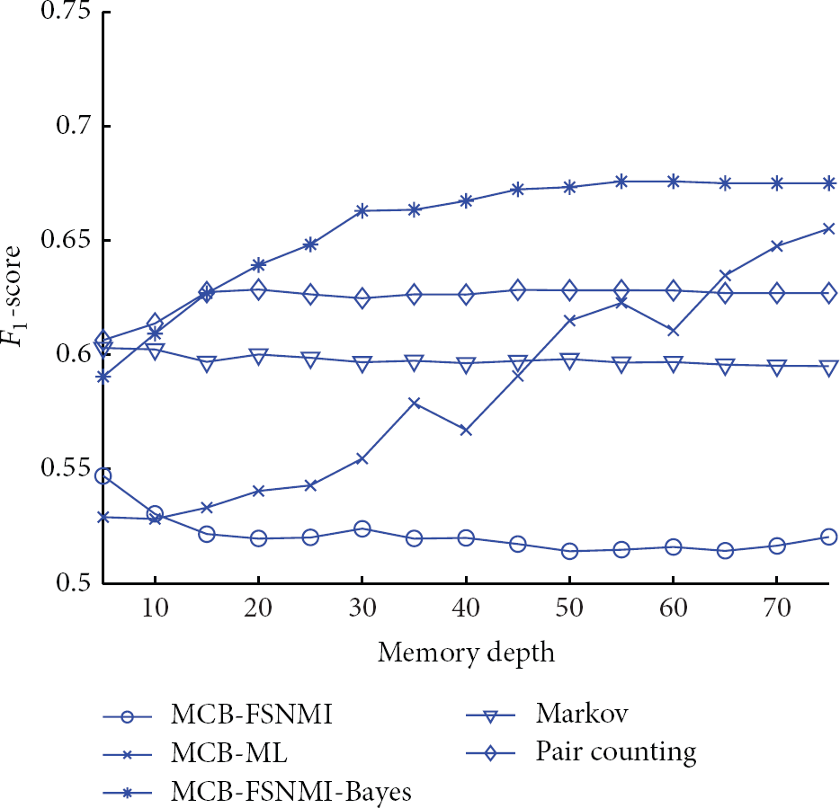
The utilization of the global history is the most important in designing the interference predictor for the CMA in the LEO satellite uplink. The memory depth is defined as the number of the memorized periods utilized for the prediction, which can represent the length of the history utilized. The dataset with a large memory depth contains the global history of interferences. Therefore, we can evaluate how well a predictor utilizes the global history by observing the change of its performance as the memory depth increases. The predictor can utilize the global history well if its performance increases dramatically and keeps increasing as the memory depth increases. In this test, we analyze for each predictor the change of the performance. We measure the performances of the different predictors given the different memory depths by the $F_1$ -score and the $F_2$ -score, respectively. The results are shown in Figures 7 and 8. The maximal memory depth is 75 since there are 75 periods in all. The minimal memory depth is 5 because we need to ensure a memory depth that is not too small for the matching algorithms. Also, the Markovian method reaches its best at the memory depth of 5. As suggested in test (Section 4.1), the packet size is set to be 2 for MCB-FSNMI, MCB-ML, MCB-FSNMI-Bayes, and the pair counting-based method. The predefined threshold of the Markovian method is set to be optimal regarding the $F_1$ -score and the $F_2$ -score.

Figure 7

Comparisons under the different memory depths by the $F_1$ -score.

Figure 8

Comparisons under the different memory depths by the $F_2$ -score.

As shown in Figures 7 and 8, the difference between the results evaluated by the $F_1$ -score and the $F_2$ -score is not obvious. The results in both of the figures are analyzed together. In Figures 7 and 8, the pair counting-based method works better than MCB-ML and MCB-FSNMI-Bayes when the memory depth is no larger than 60 and 15, respectively. Its performance increases dramatically when the memory depth is no larger than 15. However, its performance gets bounded when the depth is only 15. This can be reasoned by the characteristic of the matching algorithm. The memorized periods of the pair counting-based method contain all the samples in the periods, which may cover the useful information with the noisy data. Then, the different periods may seem similar to each other with the noise. Therefore, the pair counting-based method is too simple to effectively distinguish the difference between two similar memorized periods. It can also tell us that the storing of all the samples is neither efficient nor effective for our problem.

MCB-ML works poorly when the memory depth is no larger than 40. However, its performance is improved dramatically as the memory depth increases. Finally, it is the second best among all the predictors when the memory depth is no less than 65. The scheme works poorly given a small memory depth because it is designed by the maximum likelihood criterion. The likelihood in matching the different memorized periods may be close to each other if there is no prior information and the memory depth is small. Thus, the error could happen when the likelihood is used for the matching and the corresponding prediction. It is well known that the maximum likelihood algorithm always works poorly when the dataset is not big enough. The predictor could be misled by the data before the correct information is obtained from a large dataset. Therefore, it can be concluded that MCB-ML can utilize the global history, but its performance is constrained by the size of the dataset seriously. MCB-ML cannot perform well when the memory depth is not large enough. Even if the memory depth is 75, it is still inferior to MCB-FSNMI-Bayes since the Bayesian method can be assisted by the prior information.

MCB-FSNMI works poorly when the memory depth is 5, and it works even more poorly as the memory depth increases. The scheme cannot distinguish the different memorized periods effectively. As analyzed in test (Section 4.1), it is improper to use FSNMI alone for the matching and the corresponding prediction.

It is better to use FSNMI as the assistant information for the other schemes. For example, we combine FSNMI with MCB-ML to obtain the Bayesian scheme MCB-FSNMI-Bayes. The scheme is inferior to the pair counting-based method when the memory depth is no larger than 15. But its performance can increase dramatically in Figures 7 and 8 when the memory depth is no larger than 30. And it still keeps increasing slowly when the memory depth is even larger. Compared with MCB-ML, its performance is much better when the memory depth is less than 45. The reason is that the scheme can avoid the misleading of the small dataset by utilizing the prior information FSNMI. And, even if the memory depth is 75, the scheme still works better than MCB-ML. MCB-FSNMI-Bayes is the best of all when the memory depth is larger than 15 since it can utilize both the global history and the samples collected in the initial scan as a whole.

The Markovian method is better than MCB-FSNMI-Bayes and MCB-ML when the memory depth is no larger than 5 and 45, respectively. However, its performance cannot be improved as the memory depth gets larger. On the contrary, the performance gets even slightly worse when more memorized periods are used for the statistics. The Markovian method cannot utilize the global history and the performance is not desirable as the memory depth increases. This is because the method always assumes the constant parameters and thus it cannot deal with global history of the interferences.

4.3. Probability of Detection and the Spectrum Loss Rate

The performances of the predictors have been evaluated by the $F_1$ -score and the $F_2$ -score. It has been validated that the scheme MCB-FSNMI-Bayes can utilize the global history and outperforms the others with a memory depth larger than 15. These tests evaluate both $P_d$ and $P_{\text{fa}}$ at the same time. However, there may be some specific requirements of $P_d$ or SLR. The measure $P_d$ represents the success rate of the interference prediction. Sometimes, we may need to assure a higher quality of the communication services. In this case, a higher $P_d$ is required. SLR measures how much of the spectrum is wasted due to the false alarm, though $P_{\text{fa}}$ is important and it has been included in calculating the $F_p$ -score. Sometimes, we may need to occupy more bandwidth to achieve a higher communication rate. In this case, a lower SLR is required. Therefore, we need to further evaluate the performances under the specific requirement of $P_d$ or SLR.

We evaluate the overall performances of the predictors with the $F_p$ -score under the different requirements. When two predictors are compared and adjusted to meet a specific requirement, the one that has a higher $F_p$ -score is the better one. In Figures 9 and 10, MCB-FSNMI-Bayes and the Markovian method are compared under the different requirements of $P_d$ and SLR, respectively. In Figures 11 and 12, we compare MCB-FSNMI-Bayes with the pair counting-based method in the same way. Among the MCB schemes, we only evaluate MCB-FSNMI-Bayes here, because it has been validated that the scheme has an advantage over MCB-ML and MCB-FSNMI by combining them both. The parameter p of the $F_p$ -score is just set as 1 here, since the difference between the results evaluated by the $F_1$ -score and the $F_2$ -score is not obvious in the above tests.

Figure 9

Comparison of MCB-FSNMI-Bayes and the Markovian method by the $F_1$ -score and $P_d$ .

Figure 10

Comparison of MCB-FSNMI-Bayes and the Markovian method by the $F_1$ -score and 1-SLR.

Figure 11

Comparison of MCB-FSNMI-Bayes and the pair counting-based method by the $F_1$ -score and $P_d$ .

Figure 12

Comparison of MCB-FSNMI-Bayes and the pair counting-based method by the $F_1$ -score and 1-SLR.

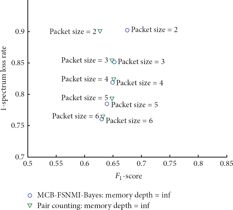
The values on the Y-axis of Figures 9 and 11 represent $P_d$ , and the values on the Y-axis of Figures 10 and 12 represent 1-SLR. The measure 1-SLR reaches its best value at 1 and worst value at 0. The values on the X-axis of Figures 9–12 represent the $F_1$ -score. In Figures 9–12, a data point in the northeast of the figures represents a better performance than a data point in the southwest does. When two data points have the same value on the Y-axis, the data point that has a greater value on the X-axis performs better.

The memory depths of the predictors are set to be optimal according to the results in test (Section 4.2). The memory depths of both the MCB-FSNMI-Bayes and the pair counting-based method are set as infinite. It is because the performances will not get deteriorated as the memory depth increases. But the memory depth of the Markovian method is set to be 5, since the method cannot utilize the global history and its performance gets slightly worse as the memory depth increases. For MCB-FSNMI-Bayes and the pair counting-based method, the different $P_d$ or SLR is adjusted by setting the different packet size. For the Markovian method, the predefined threshold is set for the adjustment.

As shown in Figure 9, MCB-FSNMI-Bayes has a higher $F_1$ -score than the Markovian method when both of the methods can achieve the same $P_d$ . It means that the Markovian method needs to produce more false alarm than MCB-FSNMI-Bayes to achieve the same $P_d$ . As shown in Figure 10, the data points that represent the performances of MCB-FSNMI-Bayes are to the northeast of the data points that represent the performances of the Markovian method. Hence, MCB-FSNMI-Bayes outperforms the Markovian method obviously when there is a specific requirement of the SLR. The Markovian method is more likely to produce false alarms and thus lead to a lower 1-SLR.

It can be concluded from the results in Figures 9 and 10 that MCB-FSNMI-Bayes has a better performance than the Markovian method under the specific requirement of $P_d$ or the SLR. As shown in Section 4.2, MCB-FSNMI-Bayes can utilize the global history while the Markovian method cannot. So, the overall performance of the Markovian method is worse, and the method needs to improve its $P_d$ at the cost of enormously increasing its SLR.

We also compare MCB-FSNMI-Bayes with the pair counting-based method in the same way. The results in Figures 11 and 12 also show that MCB-FSNMI-Bayes has a higher $F_1$ -score than the pair counting-based method when there is a specific requirement of $P_d$ or SLR. Therefore, it can be concluded that MCB-FSNMI-Bayes is superior to the pair counting-based method to meet the different requirements of $P_d$ or SLR. Moreover, the pair counting-based method needs to unrealistically store the complete dataset of the memorized periods. So, compared with MCB-FSNMI-Bayes, the pair counting-based method is neither efficient nor effective. It is because the pair counting-based method is disturbed by the noisy data as explained in Section 4.2.

5. Conclusion

The onboard interference prediction for the CMA in the LEO satellite uplink transmission is difficult because of the global history of interferences and the limited onboard storing capability of the LEO satellite. Moreover, a long-term interference prediction is important for the LEO satellite to avoid the expensive overhead of the frequent spectrum handoff. In this study, we design the MCB scheme that can efficiently utilize the global history by SSD for the prediction. There are three different MCB schemes with the different matching algorithms. Among the MCB schemes, the best one is MCB-FSNMI-Bayes that can treat the samples collected in the initial scan as whole and utilize the proposed prior information FSNMI as well. The different MCB schemes are also compared with the pair counting-based method and the Markovian method. Compared with MCB-FSNMI-Bayes, the pair counting-based method is neither effective nor efficient, and the Markovian method can only utilize the local history of interferences rather than the global one. So, the proposed method MCB-FSNMI-Bayes is the most proper scheme for the interference prediction here. All these conclusions are validated experimentally with the real interference data that were collected by an LEO satellite. The experiments on the real data assure that the proposed schemes are suitable for the practical use.