Online Bayesian Data Fusion in Environment Monitoring Sensor Networks

Abstract

Assuring reliable data collection in environment monitoring sensor network is a major design challenge. This paper gives a novel Bayesian model to reliably monitor physical phenomenon. We briefly review the errors on the data transfer channel between the sensor quantifying the physical phenomenon and the fusion node, and a discrete K-ary input and K-ary output channel is presented to model the data transfer channel, where K is the number of quantification levels at the sensor. Then, discrete time series models are used to estimate the mean value of the physical phenomenon, and the estimation error is modeled as a Gaussian process. Finally, based on the transition probability of the proposed data transfer channel and the probability of the estimated value transited to specific quantification levels, the level with the maximum posterior probability is decided to be the current value of the physical phenomenon. Evaluations based on real sensor data show that significant gain can be achieved by the proposed algorithms in environment monitoring sensor networks compared with channel-unaware algorithms.

1. Introduction

Advances in wireless communication technologies together with the aggressive feature size scaling in VLSI circuits have enabled the massive deployment of ultrasmall, cost efficient, and low power sensor nodes, which have led to the blossom of wireless sensor networks (WSN) in a wide range of applications, such as environment monitoring, battlefield surveillance, health care, and home automation [1]. Common goal in most WSN applications is to reconstruct the underlying physical phenomenon (e.g., temperature and humidity), based on sensor observations [2, 3]. However, the context of WSN makes this task very challenging. First, each sensor is characterized by low power supply and limited computation and communication capabilities due to various design considerations such as small size battery, bandwidth, and cost. Second, the harsh environments where the sensor is deployed further exacerbate the reliability of sensors. Subsequently, ensuring the reliability of the data in WSN is going to be very challenging for WSN designers.

In WSN, sensor observations are exposed to various sources of errors during the course of sensing, processing, and communication. First of all, sensors may report readings with time-invariant bias known as systematic errors due to residual sensor calibration errors [4]. For example, in case of a light sensor, the biased readings can be incurred by sensor hardware or external factors such as dust particles on the protective lens of the sensor. After sensing and quantization, the data can still be disturbed by various soft errors on chips caused by thermal noise and cosmic ray radiations [5]. Afterward, the data samples again suffered from the wireless channel errors during the data reporting to sink node [6]. These kinds of errors are different in terms of severity, occurrence rates, and statistics.

Various error control strategies designed to control different errors for WSN have been investigated extensively in the literatures. Recently, schemes can calibrate single-sensor system biases by tuning each individual sensor based on ground truth information and advanced collaborative schemes can handle system biases for large scale of sensors which have been proposed in [7, 8], respectively. To tackle soft errors on chip and channel errors, majority of the existing methods have been turned to introduce redundancy to handle these kinds of errors individually. For example, error correction codes (ECC) and triple modular redundancy (TMR) [9] have been used widely to control soft errors on chips. Similarly, ECC together with automatic retransmission requests (ARQ) [10] have been applied to control wireless channel errors.

All the aforementioned algorithms address the reliable data reception problem by either introducing redundancies or fitting statistical models of the monitored phenomena but ignore the data transfer channel (DTC) error information. Due to the promise of considerable performance improvements as has been proved in decision fusion [11, 12], target tracking [13], and multiple accesses [14] scenarios, channel-awareness related algorithms have attracted wide interest. In this paper, we focus on the reliable data reception from a sensor node that quantizes the monitored phenomenon into K levels, which is the basic problem for WSNs. We wish to design a decision device which chooses a quantization level for the current phenomenon such that the probability of a correct decision is maximized. Both the temporal correlation of a physical phenomenon and the error information of the DTC are modeled as prior input to the decision device.

The rest of the paper is organized as follows. Section 2 introduces the system model of data reception at the sink node from a sensor node. Section 3 models the error-prone DTC by a discrete K-ary input and K-ary output channel, where K is the number of quantization levels. Then, a discrete time series model is used to estimate the value of the monitored physical phenomenon and the estimation error is modeled as a normal distribution in Section 4. Section 5 gives some results that demonstrate the efficiency of the proposed algorithms. Finally, conclusions and future extensions are given in Section 6.

2. System Models and Problem Formulation

The problem to be solved including the network and channel-aware Bayesian model is first described formally.

2.1. Network Model

Figure 1 depicts the typical topology of WSN. Let $\mathbf{M}=\{m_{\mathrm{1}},\dots ,m_N\}$ be a finite set corresponding to N sensor nodes observing a common phenomenon J. The gathered data sequences at the fusion node, from the observation sequences of sensor $m_n$ , are denoted by ${\{z_t^n\}}_{t=\mathrm{1}}^{\infty }$ , where t represents the time index and n is the node index. ${\{{\gamma }_t\}}_{t=\mathrm{1}}^{\infty }$ denotes the fusion decisions using the observations of all the sensor nodes in set M.

Figure 1

System model for distributed fusion.

Definition 1.

The phenomenon J is a continuous stochastic process bounded at interval $[l,u]$ and $J^t$ is the realization of J at tth transmission phase. The sensor digitalizes the interval $[l,u]$ uniformly into K quantization levels $\theta =\{{\theta }_{\mathrm{1}},\dots ,{\theta }_K\}$ , where $K={\mathrm{2}}^q\hspace{0.17em}\hspace{0.17em}(q=\mathrm{1,2},\dots )$ . Each quantization level represents a subinterval with size $\mathrm{\Delta }=(u-l)/K$ . Using ${\theta }_i^t$ denotes that ${\theta }^t={\theta }_i\hspace{0.17em}\hspace{0.17em}(i=\mathrm{1,2},\dots ,K)$ , where ${\theta }^t$ is the digitalized version of $J^t$ at tth transmission phase.

2.2. Bayesian Data Reliability Model

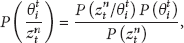
As shown in Figure 1 at time t, the sensor node $m_n$ sampled and quantified the observation as phenomenon J. After sensing and quantization, the observation is reported to the fusion node. After receiving the data reporting from sensor node $m_n$ , it is proposed to design a data detector that makes a decision on the received data and the error probability of the data transfer channel such that the probability of a correct decision is maximized. Using Bayes’ rule, the posterior probabilities can be expressed as

$$\begin{array}{cc}& P\left(\frac{{\theta }_i^t}{z_t^n}\right)=\frac{P\left(z_t^n/{\theta }_i^t\right)P\left({\theta }_i^t\right)}{P\left(z_t^n\right)},\end{array}$$

(1)

where $P({\theta }_i^t/z_t^n)$ are the conditional probabilities of the phenomenon ${\theta }^t={\theta }_i$ at time t, given the event that the gathered data at the fusion node from sensor node $m_n$ at time t is $z_t^n$ . The decision criterion is based on selecting the subinterval corresponding to the maximum of the set of posterior probabilities. $P({\theta }_i^t/z_t^n)$ . $P(z_t^n/{\theta }_i^t)$ are the conditional probabilities of the event that the gathered data at the fusion node from sensor node $m_n$ at time t is $z_t^n$ , given phenomenon ${\theta }^t={\theta }_i$ at time t, and $P(z_t^n/{\theta }_i^t)$ are the priori probabilities which specify the data transfer channel. $P({\theta }_i^t)$ are the probabilities of the phenomenon ${\theta }^t={\theta }_i$ at time tand are also the priori probabilities that depended on the statistic property of the phenomenon. The denominator of (1) can be expressed as

$$\begin{array}{cc}& P\left(z_t^n\right)={\displaystyle \sum }_{i=\mathrm{1}}^{K}P\left(\frac{z_t^n}{{\theta }_i^t}\right)P\left({\theta }_i^t\right).\end{array}$$

(2)

From (1) and (2), we observe that the computation of the posterior probabilities $P({\theta }_i^t/z_t^n)$ requires knowledge of the priori probabilities $P(z_t^n/{\theta }_i^t)$ and $P({\theta }_i^t)$ .

3. Data Transfer Channel Model for WSN

In Section 2, we have demonstrated that the computation of the posterior probabilities $P({\theta }_i^t/z_t^n)$ requires knowledge of the priori probabilities $P(z_t^n/{\theta }_i^t)$ , which are depended on the statistic property of the data transfer channel between the sensor of the sensor node who samples the phenomenon J and the fusion node shown in Figure 2. In this section, we first investigate the error models for the cosmic ray radiation induced errors, thermal noise on chip induced errors, and wireless channel errors. Then, we propose a discrete K-ary input and K-ary output channel to model the data transfer channel as shown in Figure 2.

Figure 2

Errors on the data transfer channel between the sensor node and fusion node within one hop.

3.1. Model for Radiation Induced Transient Error

When a radioactive particle strikes a semiconductor device, it causes a transient pulse that may alter the logical state of the struck node. The generated transient glitches on the circuit can be propagated through the circuit and reversed value gets latched into sequential circuit and becomes an error. Soft error rate (SER) of a circuit is exponentially related to the critical charge $Q_{\text{CRIT}}$ , which is the minimum charge required to cause a soft error and is proportional to system supply voltage:

$$\begin{array}{cc}& P_{\text{ser}}\propto F·A·\exp \left(-\frac{Q_{\text{CRIT}}}{Q_S}\right).\end{array}$$

(3)

F is the neutron flux (i.e., radiation intensity), which is related to the environment where the device operates. A is the area of the circuit sensitive to particle strikes. $Q_S$ is the charge collection efficiency of the device. According to [5]

$$\begin{array}{cc}& Q_{\text{CRIT}}\propto V_{dd}.\end{array}$$

(4)

$V_{dd}$ is system supply voltage. As shown in (4), when supply voltage decreases the critical charge decreases, which will increase the transient error rate. Besides, the flux of low energy particles is orders of magnitude higher than high energy particles [15]. Therefore, with smaller critical charge, circuits are more vulnerable to transient errors induced by lower energy particle strikes.

3.2. Model for Thermal Noise Induced Transient Error

Thermal noise in logic gates is a stationary Gaussian stochastic voltage fluctuation process with zero mean value and deviation ${\delta }_N=\kappa T$ , where κ is the Boltzmann constant and T is the temperature [16]. The model of logic gate considered herein is shown in Figure 2 and was first used by author [17]. It consists of three cascaded stages. The first stage is the logic function, which is used to compute the true value of the logic gate. The next stage is the additive white Gaussian noise (AWGN) channel, which is the noise channel when the logic value transfers through the logic gate. The essence of this stage is to add thermal noise to the data transferred from the input to output. The third is a threshold function, which restores binary data readout from the logic gate. Whenever the noise voltage exceeds the threshold value $V_{\text{th}}$ of the logic gate, an error will happen. Clearly, the logic gate, through which data is transferred, can be modeled as a binary symmetric channel (BSC) [5]. The bit error rate (BER) of the BSC channel is $P_{\epsilon }$ :

$$\begin{array}{cc}& P_{\text{noise}}=\frac{\mathrm{1}}{\mathrm{2}}\mathrm{erfc}\left(\sqrt{\frac{V_{\text{th}}}{\kappa T}}\right),\end{array}$$

(5)

where $\mathrm{erfc}(\gamma )=(\mathrm{2}/\sqrt{\pi }){\int }_{\gamma }^{\infty }\exp (-{\tau }^{\mathrm{2}})d\tau$ and we assume $V_{\text{th}}=(\mathrm{1}/\mathrm{2})V_{dd}$ , which is the typical case in [5].

3.3. Model for Wireless Channel Error

Since most of the envisioned applications for WSNs assume that sensor nodes are densely lying on the ground and their antennas are a few centimeters over the ground, this near ground feature makes the channel models for WSNs to be different from the channel models used in mobile wireless communication networks, where antennas are always over the ground by 1.5 meters. Many field measurement campaigns have verified and reported that one and two slope log distance path loss models are suitable for near ground channel for WSNs deployed in outdoor scenarios [18]. Comparing to one-slope log-distance path loss model, two-slope log-distance path loss model can provide lower model error at 868 MHZ in ISM band. Because most of the radio energy is intercepted by the ground within the Fresnel zone, the path loss exponent will be bigger than the path loss exponent beyond the Fresnel zone. However, considering the small size of the Fresnel zone, we think one-slope log-distance path loss, which can be fitted by the measurements beyond the Fresnel zone, can accurately model the channel for WSNs:

$$\begin{array}{cc}& L\left(d\right)=\text{PL}\left(d_{\mathrm{0}}\right)+\mathrm{10}\eta \hspace{0.17em}\text{lo}{\text{g}}_{\mathrm{10}}\left(\frac{d}{d_{\mathrm{0}}}\right)+X_{\sigma },\end{array}$$

(6)

where $\text{PL}(d_{\mathrm{0}})$ is the path loss at a reference distance $d_{\mathrm{0}}$ in dB, η is the path loss exponent, and $X_{\sigma }$ denotes the shadowing fading component, with $X_{\sigma }~N(\mathrm{0},\sigma )$ .

Definition 2.

Equation (6) can accurately model the one-hop channel between two sensors within WSNs. $h(d)$ is the one-hop channel response in frequency domain for the two sensors at distance d apart.

Based on Definition 2, we define an intermediate variable called channel fading factor $h^{\prime }(d)=\mathrm{10}\hspace{0.17em}\text{lo}{\text{g}}_{\mathrm{10}}(\parallel h(d)\parallel )$ , which measures the amplitude of $h(d)$ in dB:

$$\begin{array}{cc}& h^{\prime }\left(d\right)=L\left(d\right)=\text{PL}\left(d_{\mathrm{0}}\right)+\mathrm{10}\eta \hspace{0.17em}\text{lo}{\text{g}}_{\mathrm{10}}\left(\frac{d}{d_{\mathrm{0}}}\right)+X_{\sigma }.\end{array}$$

(7)

Definition 3.

The additive Gaussian noise at the receiver is $n~N(\mathrm{0},\sqrt{N_{\mathrm{0}}/\mathrm{2}})$ . We further assume that the sensor nodes transmit binary PAM signals, where the two signals waveforms are $s_{\mathrm{1}}=\sqrt{{\epsilon }_b}$ and $s_{\mathrm{2}}=-\sqrt{{\epsilon }_b}$ in the signal duration intervals and zero elsewhere. The two signals are equally likely to be transmitted.

Theorem 4.

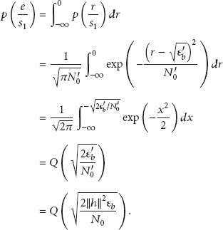
If Definitions 2 and 3 hold, the probability of error between one hop is

$$\begin{array}{cc}& P_{hop}=Q\left(\sqrt{\frac{\mathrm{2}{\parallel h\parallel }^{\mathrm{2}}{\epsilon }_b}{N_{\mathrm{0}}}}\right).\end{array}$$

(8)

Proof.

Let us assume $s_{\mathrm{1}}$ is transmitted. Then, the received signal from the demodulator is

$$\begin{array}{cc}& r={\parallel h\parallel }^{\mathrm{2}}{s}_{\mathrm{1}}+h^{*}n=\sqrt{{\epsilon }_b^{\prime }}+n^{\prime },\end{array}$$

(9)

where ${\epsilon }_b^{\prime }={\parallel h\parallel }^{\mathrm{4}}{\epsilon }_b$ , $n^{\prime }~N(\mathrm{0},\sqrt{N_{\mathrm{0}}^{\prime }/\mathrm{2}})$ ,   $N_{\mathrm{0}}^{\prime }={\parallel h\parallel }^{\mathrm{2}}{N}_{\mathrm{0}}$ . The optimal decision is made by the following rules:

$$\begin{array}{cc}& p\left(\frac{r}{s_{\mathrm{1}}}\right)\ge p\left(\frac{r}{s_{\mathrm{2}}}\right)\hspace{1em}r=s_{\mathrm{1}}\\ p\left(\frac{r}{s_{\mathrm{1}}}\right)<p\left(\frac{r}{s_{\mathrm{2}}}\right)\hspace{1em}r=s_{\mathrm{2}}.\end{array}$$

(10)

The two conditional pdfs of r are

$$\begin{array}{cc}& p\left(\frac{r}{s_{\mathrm{1}}}\right)=\frac{\mathrm{1}}{\sqrt{\pi N_{\mathrm{0}}^{\prime }}}\exp \left(-\frac{{\left(r-\sqrt{{\epsilon }_b^{\prime }}\right)}^{\mathrm{2}}}{N_{\mathrm{0}}^{\prime }}\right)\\ p\left(\frac{r}{s_{\mathrm{2}}}\right)=\frac{\mathrm{1}}{\sqrt{\pi N_{\mathrm{0}}^{\prime }}}\exp \left(-\frac{{\left(r+\sqrt{{\epsilon }_b^{\prime }}\right)}^{\mathrm{2}}}{N_{\mathrm{0}}^{\prime }}\right).\end{array}$$

(11)

Given that $s_{\mathrm{1}}$ is transmitted, the probability of error is simply the probability that $r<\mathrm{0}$ ; that is,

$$\begin{array}{l}p\left(\frac{e}{s_{\mathrm{1}}}\right)={{\displaystyle \int }}_{-\infty }^{\mathrm{0}}p\left(\frac{r}{s_{\mathrm{1}}}\right)dr\hfill \\ =\frac{\mathrm{1}}{\sqrt{\pi N_{\mathrm{0}}^{\prime }}}{{\displaystyle \int }}_{-\infty }^{\mathrm{0}}\exp \left(-\frac{{\left(r-\sqrt{{\epsilon }_b^{\prime }}\right)}^{\mathrm{2}}}{N_{\mathrm{0}}^{\prime }}\right)dr\hfill \\ =\frac{\mathrm{1}}{\sqrt{\mathrm{2}\pi }}{{\displaystyle \int }}_{-\infty }^{-\sqrt{\mathrm{2}{\epsilon }_b^{\prime }/N_{\mathrm{0}}^{\prime }}}\exp \left(-\frac{x^{\mathrm{2}}}{2}\right)dx\hfill \\ =Q\left(\sqrt{\frac{\mathrm{2}{\epsilon }_b^{\prime }}{N_{\mathrm{0}}^{\prime }}}\right)\hfill \\ =Q\left(\sqrt{\frac{\mathrm{2}{\parallel h\parallel }^{\mathrm{2}}{\epsilon }_b}{N_{\mathrm{0}}}}\right).\hfill \end{array}$$

(12)

Similarly, if we assume that $s_{\mathrm{2}}$ is transmitted, the received signal from the demodulator is

$$\begin{array}{cc}& r={\parallel h\parallel }^{\mathrm{2}}{s}_{\mathrm{2}}+h^{*}n=-\sqrt{{\epsilon }_b^{\prime }}+n^{\prime }.\end{array}$$

(13)

Given that $s_{\mathrm{2}}$ is transmitted, the probability of error is simply the probability that $r>\mathrm{0}$ ; that is,

$$\begin{array}{cc}& p\left(\frac{e}{s_{\mathrm{2}}}\right)={{\displaystyle \int }}_{-\infty }^{\mathrm{0}}p\left(\frac{r}{s_{\mathrm{2}}}\right)dr=Q\left(\sqrt{\frac{\mathrm{2}{\parallel h\parallel }^{\mathrm{2}}{\epsilon }_b}{N_{\mathrm{0}}}}\right).\end{array}$$

(14)

Based on (10) and (12), the probability of error between one hop is as follows like (8):

$$\begin{array}{cc}& P_{\text{hop}}=\frac{\mathrm{1}}{\mathrm{2}}p\left(\frac{e}{s_{\mathrm{1}}}\right)+\frac{\mathrm{1}}{\mathrm{2}}p\left(\frac{e}{s_{\mathrm{2}}}\right)=Q\left(\sqrt{\frac{\mathrm{2}{\parallel h\parallel }^{\mathrm{2}}{\epsilon }_b}{N_{\mathrm{0}}}}\right).\end{array}$$

(15)

Theorem 5.

Figure 3 shows the model for data transmission over an end-to-end link in F-hop WSNs with $F-1$ amplify-and-forward (AF) relay nodes, where $F\ge \mathrm{2}$ . If Definitions 2 and 3 hold, the bit error probability of the DTC in F-hop WSNs is

$$\begin{array}{cc}& P_{hop}\le Q\left(\sqrt{\frac{\mathrm{2}{\parallel h_F^t\parallel }^{\mathrm{2}}{\epsilon }_b}{N_{\mathrm{0}}{\left(\mathrm{1}+{\sum }_{f=\mathrm{1}}^{F-\mathrm{1}}\parallel h_F^t/h_f^t\parallel \right)}^{\mathrm{2}}}}\right),\end{array}$$

(16)

where $h_f^t,s_f^t$ , and $r_f^t$ denote the channel response of the fth hop, the transmitted, and received signal by the fth relay node in the tth transmission phase, respectively. Particularly, $s_{\mathrm{0}}^t$ and $r_F^t$ are, respectively, the transmitted signal by the sensor node and received signal at the sink node in the tth transmission phase.

Figure 3

Model for data transmission over an end-to-end link in F-hop WSNs with $F-1$ AF relay nodes.

Proof.

First, we define that the fth relay node scales the received signal by a factor $g_f^t=\mathrm{1}/\parallel h_f^t\parallel$ at the transmission phase t. As shown in Figure 3, the received signal at the sink node in the tth transmission phase is $r_F^t=h_F^t{s}_{F-\mathrm{1}}^t+n_{\mathrm{0}}$ and the transmitted signal of this hop in this transmission phase is $s_{F-\mathrm{1}}^t=g_{F-\mathrm{1}}^t{r}_{F-\mathrm{1}}^t$ ; then,

$$\begin{array}{cc}& r_F^t=h_F^t{g}_{F-\mathrm{1}}^t{r}_{F-\mathrm{1}}^t+n_{\mathrm{0}}.\end{array}$$

(17)

The received signal of the first relay node in the tth transmission phase is

$$\begin{array}{cc}& r_{\mathrm{1}}^t=h_{\mathrm{1}}^t{s}_{\mathrm{0}}^t+n_{\mathrm{0}}.\end{array}$$

(18)

Based on (17) and (18), the received signal at the sink node in the tth transmission phase is

$$\begin{array}{cc}& r_F^t=s_{\mathrm{0}}^t{\displaystyle \prod }_{f=\mathrm{1}}^F{h}_f^t{g}_{f-\mathrm{1}}^t+n_{\mathrm{0}}{\displaystyle \sum }_{f=\mathrm{2}}^F\hspace{0.17em}{\displaystyle \prod }_{m=f}^F{h}_m^t{g}_{m-\mathrm{1}}^t+n_{\mathrm{0}},\end{array}$$

(19)

where $g_{\mathrm{0}}^t=\mathrm{1}$ plug the scale factor $g_f^t$ into (19); the received signal at the sink node in the tth transmission phase can be expressed as

$$\begin{array}{cc}& r_F^t=s_{\mathrm{0}}^t{\displaystyle \prod }_{f=\mathrm{1}}^F{h}_f^t\frac{\mathrm{1}}{\parallel h_{f-\mathrm{1}}^t\parallel }+n_{\mathrm{0}}{\displaystyle \sum }_{f=\mathrm{2}}^F\hspace{0.17em}{\displaystyle \prod }_{m=f}^F{h}_m^t\frac{\mathrm{1}}{\parallel h_{m-\mathrm{1}}^t\parallel }+n_{\mathrm{0}}.\end{array}$$

(20)

Clearly, the second term of (20) can be upper-bounded by

$$\begin{array}{cc}& n_{\mathrm{0}}{\displaystyle \sum }_{f=\mathrm{2}}^F\hspace{0.17em}{\displaystyle \prod }_{m=f}^F{h}_m^t\frac{\mathrm{1}}{\parallel h_{m-\mathrm{1}}^t\parallel }\le n_{\mathrm{0}}{\displaystyle \sum }_{f=\mathrm{1}}^{F-\mathrm{1}}\parallel \frac{h_F^t}{h_f^t}\parallel .\end{array}$$

(21)

Based on (20) and (21), using LS demodulator, the bit error probability of F-hop WSNs is (16).

3.4. Data Transfer Model for WSN

Observing (3), (5), and (8), the reliability of data transfer between any two sensor nodes within one hop is determined by the soft error rate induced by the cosmic ray radiation, bit error rate induced by the on chip thermal noise, and error probability of one-hop transmission as shown in Figure 2. Furthermore, all of the three kinds of errors are related to the power supply voltage. Given the power supply voltage, the above three kinds of errors are independent with each other. For data transfer from the sensor of the sensor node who samples the phenomenon J and the fusion node within one hop, the bit error probability is

$$\begin{array}{cc}& P_b=P_{\text{ser}}+P_{\text{noise}}+P_{\text{hop}}.\end{array}$$

(22)

Then, on the same data transfer channel, the data error probability is

$$\begin{array}{cc}& P_d=\mathrm{1}-{\left(\mathrm{1}-P_b\right)}^q,\end{array}$$

(23)

where q is the number of bits in one data sample as defined in Definition 1. Since the sensor node quantifies the phenomenon J into K subintervals $\mathbf{\theta }=\{{\theta }_{\mathrm{1}},\dots ,{\theta }_K\}$ as in Definition 1, we can use the discrete K-ary input and K-ary output channel shown in Figure 4 to model the data transfer channel between the sensor of sensor node who samples the phenomenon J and the fusion node shown in Figure 2. The channel model shown in Figure 4 is characterized by the following conditional probabilities:

$$\begin{array}{cc}& P_d\left(\frac{{\theta }_j}{{\theta }_i}\right)={\left(P_b\right)}^{\text{dis}\left({\theta }_j,{\theta }_i\right)}{\left(\mathrm{1}-P_b\right)}^{m-\text{dis}\left({\theta }_j,{\theta }_i\right)},\end{array}$$

(24)

where $\text{dis}({\theta }_j,{\theta }_i)$ is the Hamming distance between the binary representation of ${\theta }_j$ and ${\theta }_i$ , which are, respectively, the jth and ith subintervals of the discrete K-ary input and K-ary output channel. $P_d({\theta }_j/{\theta }_i)$ is the conditional probability of the event that the output of the channel is ${\theta }_j$ , given the event that the input is ${\theta }_i$ .

Figure 4

Model for the data transfer channel between the sensor of the sensor node who samples the phenomenon J and the fusion node.

4. Data Source Model for Physical Phenomenon

From (1) and (2) in Section 2, we observe that the computation of the posterior probabilities $P({\theta }_i^t/z_t^n)$ requires knowledge of the priori probabilities $P({\theta }_i^t)$ , which are depended on the statistic property of the phenomenon J. In this section, we first investigate methods to model the data source of the phenomenon J. Then, methods to update the parameters of data source models online are provided to ensure robustness.

Consider an environment monitoring scenario where the sink node needs to continuously reconstruct the data field based on the data gathered from all the sensor nodes spatially and temporally correlated. That is data at any given point in such a field are correlated not only with the data at nearby points but also with the previous values of the data measured at the same point.

4.1. Empirical Model for Data Source

Models to explore the spatial and temporal correlation of a physical phenomenon are investigated in [13]. As in [13], the quantization is assumed to be very fine, and the quantization error is ignored. If at time $t_{\mathrm{2}}$ , the sink node uses the data value gathered at the point $x_{\mathrm{1}}$ and time $t_{\mathrm{1}}$ to estimate the current value at point $x_{\mathrm{2}}$ , the corresponding mean square error is assumed as follows:

$$\begin{array}{cc}& D\left(x_{\mathrm{1}},t_{\mathrm{1}};x_{\mathrm{2}},t_{\mathrm{2}}\right)=\mathrm{2}-\mathrm{2}\exp \left(-\alpha {\left(x_{\mathrm{1}}-x_{\mathrm{2}}\right)}^{\mathrm{2}}-\beta {\left(t_{\mathrm{1}}-t_{\mathrm{2}}\right)}^{\mathrm{2}}\right).\end{array}$$

(25)

In (25), the spatial distortion is related to $\left|x_{\mathrm{1}}-x_{\mathrm{2}}\right|$ , and the temporal distortion is related to $\left|t_{\mathrm{1}}-t_{\mathrm{2}}\right|$ . α and β are the spatial and temporal correlation parameters, and higher values of these parameters specify weaker correlated field. In this section, we focus on the prediction of the current value ${\theta }^t$ using the historically gathered data ${\{{\theta }^{t-\tau }\}}_{\tau =\mathrm{1}}^{\tau =w-\mathrm{1}}$ at the same location and make the following definitions.

Definition 6.

Define the prediction function as $F(·)$ . The estimation of the current value ${\theta }^t$ is denoted by ${\stackrel{-}{\theta }}^t$ , and then

$$\begin{array}{cc}& {\stackrel{-}{\theta }}^t=F\left({\left\{{\theta }^{t-\tau }\right\}}_{\tau =\mathrm{1}}^{\tau =w-\mathrm{1}}\right).\end{array}$$

(26)

We further define the ${\ell }_t={\theta }^t-{\stackrel{-}{\theta }}^t$ as the prediction error.

Time series models F are used for the prediction of the future behavior of variables. These models account for the fact that observations have an internal structure (e.g., autocorrelation, trend, or seasonal variation) that should be accounted for. Two commonly used forms of these models are autoregressive models (AR) and moving average (MA) models.

Definition 7.

The distribution of the prediction error ${\ell }_t$ is a normal distribution, with ${\ell }_t~N(\mathrm{0},{\delta }^{\mathrm{2}})$ .

Based on Definitions 6 and 7, we can give the data source model for the phenomenon J as shown in Figure 5. Denote $P_{\theta }({\theta }_i^t/{\stackrel{-}{\theta }}_k^t)$ as the probability of occurrence of the event that the current data gathered from sensor node $m_n$ is ${\theta }_i^t$ under the condition that ${\stackrel{-}{\theta }}^t={\theta }_k$ .

$$\begin{array}{l}{P}_{\theta }\left(\frac{{\theta }_i^t}{{\stackrel{-}{\theta }}_k^t}\right)=\frac{\mathrm{1}}{\delta \sqrt{\mathrm{2}\pi }}{{\displaystyle \int }}_{{\theta }_i-\mathrm{\Delta }/\mathrm{2}}^{{\theta }_i+\mathrm{\Delta }/\mathrm{2}}\exp \left(-\frac{\left(x-{\theta }_k\right)}{\mathrm{2}{\delta }^{\mathrm{2}}}\right)dx\hfill \\ =\frac{\mathrm{1}}{\sqrt{\mathrm{2}\pi }}{{\displaystyle \int }}_{\left({\theta }_i-{\theta }_k-\mathrm{\Delta }/\mathrm{2}\right)/\delta }^{\left({\theta }_i-{\theta }_k+\mathrm{\Delta }/\mathrm{2}\right)/\delta }\exp \left(-\frac{z^{\mathrm{2}}}{\mathrm{2}}\right)dz\hfill \\ =Q\left(\frac{\left({\theta }_t-{\theta }_k+\mathrm{\Delta }/\mathrm{2}\right)}{\delta }\right)-Q\left(\frac{\left({\theta }_t-{\theta }_k-\mathrm{\Delta }/\mathrm{2}\right)}{\delta }\right).\hfill \end{array}$$

(27)

Given ${\theta }^{t-\mathrm{1}}={\theta }_k$ , we observe that the parameter $P_{\theta }({\theta }_i^t)$ of the Bayesian model (1) is equal to $P_{\theta }({\theta }_i^t/{\theta }_k^{t-\mathrm{1}})$ as shown in Figure 5. This empirical model is characterized by one parameter δ to be determined. Comparing to (25), we know that $\delta \propto \beta {(t_{\mathrm{1}}-t_{\mathrm{2}})}^{\mathrm{2}}$ , where $\left|t_{\mathrm{1}}-t_{\mathrm{2}}\right|$ denotes the sample interval. In the runtime stage, we can update the parameter δ according to the observations gathered at the fusion node as $\delta =\max (\left|z_{\tau }^n-z_{\tau -\mathrm{1}}^n\right|)$ , with $\tau =t-w,\dots ,t-\mathrm{1}$ . w is the window length and is less than t.

Figure 5

Empirical data source model for phenomenon J.

4.2. Learning Model for Data Source

Beside the empirical models, we can also learn the parameter $P({\theta }_i^t)$ in the Bayesian model (1) by random experiments. That is, the fusion node needs to keep $K^{\mathrm{2}}$ counters to log the occurrences of the pair $({\theta }_k^{t-\mathrm{1}},{\theta }_i^t)$ . Learning the model parameter by training is simple. However, enough random experiments are required until the learning is reasonable.

5. Experimental Evaluations

5.1. Evaluation Setup

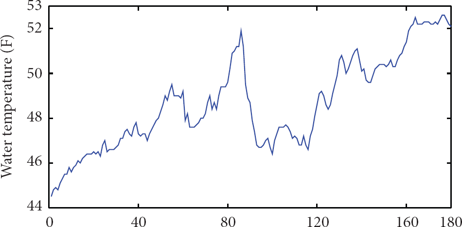
The data are quantized as 8-bit values in our evaluations, including sensor data about water temperature, dissolved oxygen in river water, and river stage from the California Data Exchange Center (CDEC) [19]. As shown in Figures 6, 7, and 8, these data sets differ in terms of autocorrelation properties and degrees of stationarity.

Figure 6

The plot of data set 1.

Figure 7

The plot of data set 2.

Figure 8

The plot of data set 3.

Most of the envisioned applications of WSNs assume that sensor nodes are densely lying on the ground and their antennas are a few centimeters over the ground. This near ground feature makes the channel in WSNs to be very different from the channel in mobile communication networks, where antennas are always over the ground by 1.5 meters. Many field measurement campaigns have verified and reported that the two-slope log-distance path loss model can accurately model the near ground channel in WSNs deployed in outdoor scenarios at ISM frequency band [20]. Considering the small Fresnel zone, we assume there are no sensor nodes locating within the Fresnel zone of the other sensor nodes, and we can use one-slope path loss model shown in (28) as the channel between the transmitter and receiver of every hop:

$$\begin{array}{cc}& \mathrm{20}\hspace{0.17em}\log \left(h\right)=L_{\mathrm{0}}+\mathrm{10}n\hspace{0.17em}\log \left(\frac{d}{d_{\mathrm{0}}}\right)+X_{\sigma },\end{array}$$

(28)

where $d_{\mathrm{0}}$ is the breakpoint, $L_{\mathrm{0}}$ is the path loss at $d_{\mathrm{0}}m$ , n is the path loss factor, d is the distance between the transmitter and receiver, and $X_{\sigma }$ is a normal random variable with standard deviation σ.

In experiments, we assume $d_{\mathrm{0}}=\mathrm{2}$  m,   $L_{\mathrm{0}}=\mathrm{70}$  dB,   $n=\mathrm{4}$ ,   $\sigma =\mathrm{6}$  dB, the output power of the transmitter is −30 dBm, the noise power at the receiver is $N_{\mathrm{0}}=-\mathrm{174}$  dBm, and there are no gains for both the antennas of the transmitter and receiver. We further assume that the relay nodes and sink node know perfect channel state information. The residual errors in the data after error corrections at the sink node are evaluated in terms of the normalized mean square error (NMSE) as follows:

$$\begin{array}{cc}& e_{\text{out}}=\sqrt{\frac{\mathrm{1}}{N}{{\displaystyle \sum }_{v=\mathrm{1}}^N\left|\frac{{\theta }^v-{\widehat{\theta }}^v}{{\theta }^v}\right|}^{\mathrm{2}}}.\end{array}$$

(29)

In (29), N is the total number of samples. An AR model is first fitted by an offline process with the Yule-Walker method [21] in our evaluations. If the order or prediction error of the fitted AR model is too large, a RHW model [22] will be used instead. At the runtime stage, the parameters of the AR and RHW models are updated by each window of observations with the Yule-Walker method [21] and the method detailed in [22], respectively. The residual errors $e_{\text{out}}$ are compared with the NMSE $e_{\text{in}}$ of the error-corrupted data received at the sink node. For example, we list the improvement factors ( $e_{\text{in}}/e_{\text{out}}$ ) of the proposed channel-aware Bayesian model in Table 1, where the sensor node directly routes the observations of the monitored phenomenon J to the sink node and the distance between the sensor node and sink node is 40 m. In Table 1, we also give the parameters of the data sets used in our evaluation.

Table 1

Data set parameters and the improvement factors of the proposed channel-aware Bayesian mode.

Data set	Location	Sampling period	Sensor type	Sample number	Data model	$e_{\text{in}}/e_{\text{out}}$
1	Lewiston	1 day	Water temperature	181	RHW	1.5
2	Balls ferry bridge	1 hour	Dissolved oxygen in river	2191	AR, 10-order	2.0
3	Rumsey bridge	1 hour	River stage	2448	AR, 4 orders	2.1

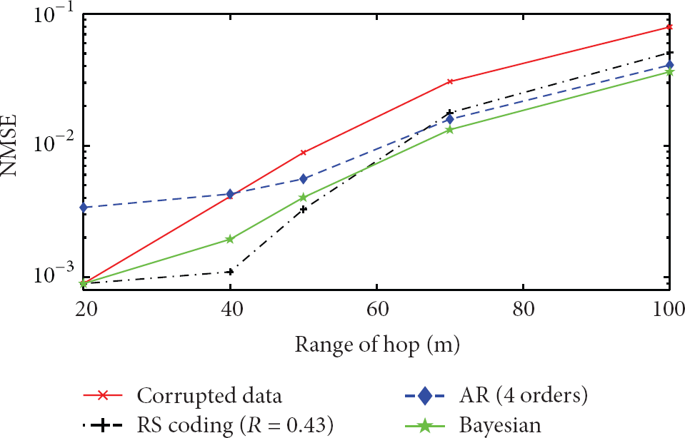
5.2. Evaluation in One-Hop WSNs

In this subsection, we evaluate the error resilience of the proposed Bayesian model, Reed-Solomon (RS) coding, and discrete time series models in one-hop WSNs, where the sensor node directly routes the observations of the monitored phenomenon J to the sink node. And the distance between the sensor node and the sink node varies from 20 m to 100 m. Figures 9, 10, and 11 compare the NMSE of the data corrected by the proposed Bayesian model and Reed-Solomon (RS) coding, and the data estimated by discrete time series models (i.e., RHW or AR models) with the NMSE of the error-corrupted data received by the sink node. In Figures 9, 10, and 11, NMSE floors of the data estimated by discrete time series models can soon be noticed, which are dominated by estimation lags around relatively fast changes of the physical phenomena. The error-corrupted data received at the sink node and data corrected by Bayesian model and RS coding show NMSE floors as well; however, these NMSE floors are much lower than the error floor of the data estimated by RHW or AR models and the common source of these NMSE floors is quantization errors. From Theorem 4 and (28), we know that the bit error probability of one-hop transmission is directly proportional to the hop distance. Due to error correction ability, the RS coding exceeds the proposed Bayesian model and discrete time series models at very low channel error levels. However, this trend is reversed in the presence of high channel error levels, because large NMSE incurred by the untreated decoding errors of RS coding in this case. The other side effect of RS coding is high communication overhead. For example, RS coding with 0.43 code rate ( $R=0.43$ ), which can nearly correct all errors at very low channel error levels, will increase the communication overhead by 57%. Unlike FEC, the overhead of the proposed Bayesian model is computation increasing at the sink node, which is caused by probabilities multiplications and can be solved by log-domain additions.

Figure 9

Evaluation in one-hop WSNs, using data set 1.

Figure 10

Evaluation in one-hop WSNs, using data set 2.

Figure 11

Evaluation in one-hop WSNs, using data set 3.

Depending on the channel error levels, the channel-aware Bayesian model will measure the quantization level with higher likelihood by more confidence. Particularly, at very low channel error levels (e.g., the distance of the hop is 20 m), the quantization levels with small distances (i.e., 0 or 1) to the channel output will have significant chance to be believed as the channel input by the channel-aware Bayesian model. Hence, at very low channel error levels the channel-aware Bayesian model performs much better than the AR and RHW models that only explore temporal correlations among observations.

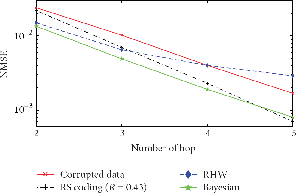
5.3. Evaluation in Multihop WSNs with Amplify-and-Forward Relay Nodes

In this subsection, we evaluate the error resilience of our model, RS coding, and discrete time series models in multihop WSNs, where the readings of the monitored phenomenon ϑ observed by the sensor node are routed to the sink node by f ( $f=\mathrm{1,2},\mathrm{3,4}$ ) relay nodes. The distance between the sensor node and the sink node is 200 m, and the distance of every hop is 200/( $f+1$ ) m. Figures 12, 13, and 14 compare the performance of our model with RS coding and discrete time series models. In the multi-hop sensor networks, where the former relay node amplifies its received signal and forwards it to the next relay node or sink node, the bit error probability of the DTC for this scenario is given by Theorem 5. Clearly as shown in both Theorem 5 and experiment results, the reliability of the end-to-end link in multihop networks degrades considerably compared with the one-hop networks with the same average distance per hop, because the amplified noise in every relay node along the transmission will finally be cumulated at the sink node. However, given a field for the coverage of WSNs, deploying more AF relay nodes still can improve the reliability of the data reception at the sink node. Similar to the results in one-hop networks, our model is still superior over the AR or RHW models and performs as well as RS coding in all cases. However, because of the increased noise level at the sink nodes in multihop networks with AF relay nodes, the performance gain of our model compared with RS coding at medium to large hop distance is increased and the performance degradation of our model at small hop distance is decreased. Moreover, like the one-hop networks, our model brings no communication overhead and the overhead of our model is computation increasing at the sink node.

Figure 12

Evaluation in multihop WSNs, using data set 1.

Figure 13

Evaluation in multihop WSNs, using data set 2.

Figure 14

Evaluation in multihop WSNs, using data set 3.

6. Conclusion and Future Works

In this paper, we have presented a channel-aware Bayesian model to reliably recover data from transient errors on the data transfer channel between the sensor node which monitors a phenomenon and the sink node, and a dis-16 crete K-ary input and K-ary output channel has been provided to formulate the error information on the data transfer channel. Using the real sensor data from CDEC, we have evaluated the performance of our method in both one-hop and multihop sensor networks. In all scenarios, the channel-aware Bayesian model is obviously superior over the discrete time series models (i.e., RHW or AR models), which merely explore the correlations among the observations of the monitored phenomena. Furthermore, the proposed channel-aware Bayesian model performs as well as the RS coding with code rate 0.43; however, the later will increase the communication overhead by 57%. Besides, RS coding can only control the wireless channel errors. The shortcoming of the channel-aware Bayesian model, which is the computation increasing caused by probability multiplications at the sink node, can be solved by log-domain algorithms.

We have identified several future research avenues. First, we currently assume that the sink node and relay nodes know perfect channel state information, and in-field model performance still needs future evaluation. Moreover, the combinations of the proposed algorithms with distributed data fusion and signal detection algorithms considering noise at the sensor of individual sensor node are the most important extensions in future.