
Abstract
In wireless sensor networks with dynamic clustering, the cluster heads are usually not selected on the basis of their locations. This causes irregular distribution of cluster heads and highly variable number of nodes in the clusters. Also, some of the clusters are spread over large areas within the network, causing limited spatial correlation between associated sensor nodes. These irregularities in cluster placements and dimensions negatively impact the efficiency of a wireless sensor network. For example, for a cooperative data aggregation, it necessitates variable or large sized packets while the aggregations, based on spatial correlation of sensor nodes, cannot be exploited easily. In this paper, we have developed a Distributed Uniform Clustering Algorithm (DUCA) for cluster based WSN. In DUCA, cluster formation mechanism is based on a virtual-grid system and sensing ranges of nodes that provide even distribution of clusters, homogenized cluster sizes, and reduced energy consumption. Simulation results show that DUCA improves the distribution of cluster heads by more than 2 times and reduces the energy consumption within a range of 15% to 50% as compared to the existing protocols.
1. Introduction
The basic job of a wireless sensor network (WSN) is to sense and collect the physical or quantifiable data from its surroundings and forward it to some central location. The central location may possibly be an isolated system or it could be a part of a globally stretched infrastructure, for example, the Internet of Things (IoT). The IoT, as envisioned, consists of data sensing and collecting objects, attached to communication devices, providing data that can be analysed and used to initiate automated actions. It has been estimated that by 2015 there will be around 25 billion devices wirelessly connected around the globe [1]. This has created a new perception of incorporating WSN as data collecting component of IoT. However, this requires much larger and wide-ranging sensor networks than currently being imagined [2]. Cooperative energy efficient data collection from such network puts new challenges on the system.
In a large scale WSN, usually, the nodes collaborate with each other to collect and forward data in a hierarchal manner. For this purpose, cluster based protocols are commonly employed. In majority of the cluster based protocols, the clusters are formed dynamically and repeatedly to collect the data from multiple sensor nodes. Usually the dynamic cluster based protocols have highly variable-sized clusters which are not formed uniformly, for example, in LEACH [3], HEED [4], EAP [5], and TDEEC [6]. By “cluster size” we mean the number of nodes in a cluster. Due to the irregular placement of sensor nodes and variable sizes of clusters, we need to have variable or large sized packets for data collection and aggregation. On the contrary, it has been shown in the previous research works that due to the limitations and resource constraints of a WSN, its optimal packet size should be small and should have fixed length [7, 8]. These packet sizes can be constrained by homogenizing cluster sizes in a WSN.
In this work our main objective is to develop a uniform cluster formation mechanism for WSNs without consuming extra energy of the network. For this purpose, we have proposed a new solution which can develop homogeneous clusters in terms of number of nodes with reduced variations in the cluster sizes. In our proposed mechanism the even distribution of cluster heads and clusters is achieved by implementing an energy efficient usage of virtual grids in the network. Unlike previously proposed grid-cluster based protocols, in our mechanism a grid is not taken as a cluster rather clusters are formed on the basis of distances of nodes to their nearest cluster heads. The sizes of clusters are further reduced by exploiting the redundant and overlapped sensing ranges, which occur due to the random placements of sensor nodes in the network.
The remaining paper is organized as follows. Section 2 further explains the problems that arise due to the highly variable sized clusters in WSNs. Section 3 gives a brief overview of the methods given in current literature to solve the problem. Section 4 explains the proposed algorithm design and compares it with the existing protocols. Section 5 discusses a heuristic approach that can be used to reduce the cluster sizes by exploiting the sensing ranges of the nodes. In Section 6, a mathematical relationship is presented that finds the optimum number of grids in the network for a given number of sensor nodes. Section 7 evaluates our proposal against centrally controlled based and grid-cluster based protocols using simulations. Finally, Section 8 concludes the paper.
2. Variable Sized Clusters in a Dynamic Cluster Based WSN
In many of the dynamic cluster based protocols like [3–6, 9–11], the location of the CHs is not considered in the CH-selection criteria. As a result, the selected CHs are not uniformly distributed in the region. For example, it can be seen in Figure 1(a) that all of the CHs are formed in the lower right corner of the network area (Figure 1(a) is a snap shot of one of the rounds taken from a simulation of LEACH protocol [3]). This type of nonuniform selection of CHs has created the following side effects on the system.
The sizes of clusters, in terms of number of nodes per cluster, are highly variable as shown in Figure 1(b). This results in the requirement of large or variable sized packets for the aggregation of data. On the other hand, due to resource constraints, the optimal packet sizes in WSNs are considered to be small and of fixed length [7, 8, 12]. There are some clusters in the network which are spread on large regions. This implies that there must be several nodes which have to contact distantly located CHs to forward their data, for example, clusters 1 and 2 in Figure 1(b). Also, the data at the CHs of these clusters must be collected from far off areas of the region. This influences the system in two ways.
The distant nodes in large sized clusters need to spend higher energy to transmit the data to their CHs. According to the free space energy consumption relation (see (1)), energy consumed in the transmission of k bit Usually in WSNs the sensor nodes placed in close vicinity have spatial correlation. Therefore, CHs after collecting data from these nodes aggregate the data into a single packet. These aggregations are usually based on simple rules of taking average, sum, difference, or maximum of the correlated data. These methods of aggregations are also called “summary based” aggregation. In large sized clusters with sensor nodes placed at far off distances, there is less chance of having good degree of spatial correlation among the data. Therefore, logical and balanced aggregation of data cannot be used easily.


Dynamic cluster based WSN.
3. Related Work
Some solutions have been proposed in the past to overcome the variations in the cluster sizes of WSN. We have divided these mechanisms into two categories:
centrally controlled cluster formation protocols; grid-cluster based protocols.
3.1. Centrally Controlled Cluster Formation Protocols
In these protocols the clusters are formed dynamically but the process is controlled centrally by the sink. For example, in Base Station Controlled Dynamic Clustering Protocol (BCDCP) [13], at the start of each round, all nodes send their current energy status to the sink. The sink chooses a set of CH candidates based on their energy levels. To get a set of clusters with approximately equal sizes, the sink runs the cluster splitting algorithm iteratively. In each iteration step the algorithm selects the CHs by maximizing the distances between the selected CHs, therefore creating uniformly placed CHs in the network. To form clusters, the nodes are associated to the CHs based on the closest distance. Once the clusters are formed, the extra nodes are handed and taken over between the two neighbour clusters in order to balance the size of the clusters. This whole process is centrally controlled by the sink node.
In LEACH-C [3] at the start of each cluster formation round, each node sends its residual energy level and location information to the sink node. The sink node selects CHs and builds clusters using the simulated annealing algorithm. Once the CHs and associated nodes are determined, the sink broadcasts CH IDs and Time Division Multiple Access (TDMA) schedules for each node. All nodes look for their IDs to be matched as the CH ID, if not matched then the nodes follow the Time Division Multiple Access (TDMA) schedule to broadcast their data. The data transmission phase of LEACH-C is identical to that of LEACH. This way the sink, knowing the global information of nodes, forms more uniform sized clusters.
Similar procedure has been adapted in Cluster-Based Energy-Efficient Data Collecting and Aggregation Protocol (CEDCAP) [14]. After receiving the knowledge of energy levels and locations of all nodes, the sink selects the CHs and their associated nodes. Like LEACH-C, here also sink provides the data transmission TDMA schedules to all nodes. But in CEDCAP, the TDMA calculated by the sink are scheduled according to the node degree control of each cluster. Based on the node degree control a set of nodes in each cluster are kept dormant for some period of time, hence reducing the redundant data transmission in the network.
Drawback. In centrally controlled cluster formation protocols in order to provide the energy and location status of nodes, all nodes should send extra overhead of control packets at the start of each round [3]. Besides, each node needs to remain in idle listening mode for a considerable time, in order to receive its CH IDs and TDMA schedules. Whether it is a single hop or a multihop network, additional communication cost is incurred. This cost further increases with the size of network or if nodes are placed at far off places in the network.
3.2. Grid-Cluster Based Protocols
Unlike centrally controlled cluster formation protocols, in grid-cluster based protocols the CH selection decisions are distributed among the nodes themselves. Therefore, it can work well in a large scale network. The basic idea of grid-cluster protocols is to divide the network area into equal sized virtual grids where each grid is considered as a cluster with one CH in each cluster [15–20]. The role of CH is rotated among different nodes within a cluster. Figure 2 depicts the grid-cluster method where every grid contains one CH. The main characteristics of the grid-cluster based protocols can be given as follows.
A grid is considered as a cluster; that is, the clusters are fixed and not dynamic. Although this method decreases the variations in sizes and locations of the clusters, due to the random deployment of nodes, it cannot create all equal sized clusters. Authors in [18] have tried to further even out this irregularity such that after setting one CH in each grid, the sizes of clusters are adjusted by handing and taking over extra nodes to and from the neighbour grids. This is done through a centralized control system and requires an extra overhead of control packets which consumes extra energy and delay in the system. Each grid contains one CH in it and the role of CH rotates among the nodes within a grid. For example, in [16, 20], there is a rotation of CHs which is based on a back-off timer. The back-off timer is calculated on the basis of residual energy levels of each node within a grid. In some of the grid-cluster protocols, the algorithm selects one CH per grid based on its energy level, while there is no rotation of CHs made until the energy of existing CH is completely depleted [17, 19].

Grid-cluster based WSN.
Drawback. Grid-cluster protocols have regularized the CH distributions, in the network, to some extent and have substantially reduced the variations in the cluster sizes. But the network energy consumed in these protocols is very high compared to a dynamic cluster based protocol. The reason behind this is that the selection of CHs is done only within a grid and not with respect to the whole network, as is done in LEACH. Therefore, this method does not give a fair selection of CH with respect to all of the nodes of the network. Another reason of high energy consumption is that the clusters are not formed on the basis of the distances to the closest CHs. Irrespective of the distance a node will always have to associate with the CH belonging to its own grid. For example, in Figure 2 in grid number 1 the nodes in the lower right corner of the grid will have to transmit their data to the distant CH in their grid, whereas there were two closer CHs available in grid number 2 and 5.
4. Proposed Solution
In this research work we have proposed a Distributed Uniform Clustering Algorithm (DUCA) to distribute the CHs evenly and to reduce the variations in cluster sizes in a dynamic cluster based WSN. In DUCA to get an even distribution of CHs, the network is divided into virtual grids. Unlike existing grid-cluster based protocols, the grids in DUCA do not represent a cluster. Our suggested CH selection and node association mechanism has substantially reduced the network energy consumptions compared to existing grid-cluster protocols and LEACH-C as a centrally controlled protocol.
4.1. Assumptions
Following are the basic assumptions made in DUCA design.
Initially a large number of equally charged sensor nodes are randomly deployed in the field and there is a sink node in the centre of the field. Each sensor node is stationary after deployment and is capable of getting its location information by the use of global positioning system or by using any other method of localization. Initially based on their locations each node is informed about their respective grid ID. Design of the DUCA is such that it does not require any change in the existing MAC layer of a dynamic cluster based protocol. All the contentions in DUCA are solved by the MAC layer proposed for LEACH protocol.
4.2. Algorithm Design
In DUCA, initially the sink decides the required number of CHs (C) in the network. To distribute the CHs evenly, network area is divided into
DUCA requires that each sensor node should know which grid it belongs to. In Section 4.2.1, we have explained the method and algorithm used to calculate the grid IDs for each node.
In DUCA, like other existing cluster based protocols, the collection of data is done in rounds, whereas the cluster formation process is divided into three phases. CH selections are done in the first two phases (explained in Sections 4.2.2 and 4.2.3, resp.) and node associations are done in the third phase (explained in Section 4.2.4). To make sure that we get at least one CH in almost every grid, more than required number of CHs are preelected in the first phase of CH election. This is done so that after going through the second phase of CH election we can get the required number of evenly distributed CHs in the field.
4.2.1. Detection of Grid IDs
Suppose the network is spread on a rectangular or square area with the dimensions of X by Y units (for the sake of simplicity, in our simulations we have assumed a square area). The sink calculates and assigns grid IDs to all sensor nodes in the network, based on the following steps.
Steps
Let G = grids in one column = grids in one row. The height and width of each grid are Based on the row number and column number of each grid, their grid IDs are calculated using the following, where i is the grid ID of ith grid:
And midpoint of ith grid can be calculated as follows:
Table 1 shows all the symbols and their meanings used in this paper.


Symbols and their definitions.

4.2.2. CH Election Phase 1
In this phase our aim is to get a fair selection of CHs to equalize the consumption of energy among all the nodes in the network. Therefore, the CHs are elected based on the number of times they have been selected in the previous rounds. For this the election method has been adopted from the LEACH protocol. According to LEACH, in every round, each node generates a random number between 0 and 1 and if the number is less than a threshold value 
Let P be the probability that almost every grid contains at least one CH after first phase of CH election; then, we have to maximize P such that
4.2.3. CH Election Phase 2
The preelected CHs in phase 1 are not evenly distributed; therefore, the aim of this phase is to get an even distribution of CHs in the network. Following are the steps taken.
Steps
All the CHs elected in phase 1 broadcast their residual energy levels and their grid IDs within their grid region. If there were more than one CH in a grid, after hearing the broadcast in Step 1, the one with the highest energy level gets itself elected automatically. The remaining CHs, belonging to the same grid, will go back into their normal node mode for this round. The elected CHs, finally, advertise their elections. This time, the broadcast range is increased to cover the nodes in the adjacent grids also. This is done because DUCA tries to get
This method gives number of CHs elected as almost equals to the number of grids in the region; that is,
4.2.4. Nodes Association Phase
The remaining nodes, after hearing CH advertisements, determine their closest CH on the basis of received signal strengths of multiple CHs. In this phase we have used a parameter, namely, Threshold Sensing Range (
Steps
Irrespective of their grid IDs, nodes broadcast their association requests to the CH, which has the shortest distance to them. In these broadcasts, the nodes also send their residual energy levels and their locations to the respective CHs. CHs calculate the distances between each of its associated nodes and select the active nodes for this round according to the algorithm shown in Algorithm 2. ASST_LIST is the list of nodes which are associated to this CH and the ACTIVE_LIST is the list of nodes which are active for this round only. The CH puts a node to either SLEEP_STATE or ACTIVE_STATE depending on
Put Decrease j from the ACTIVE_LIST Put Decrease i from the ACTIVE_LIST
4.3. Comparisons of Proposed Algorithm with Centrally Controlled and Grid-Cluster Based Protocols
The comparison analysis of DUCA with the centrally controlled and grid-cluster based protocols are given as follows.
The startup phase in centrally controlled cluster formation protocol is always more energy intensive than the distributed approach since the information from each node must be transmitted to the sink at the beginning of each round [3]. This cost of communication increases for the nodes that are far away from the sink [3]. This is not the case with our algorithm since it is based on distributed clustering method. Unlike centrally controlled protocol the CH selection decision is distributed among the nodes; therefore, the proposed algorithm can be used in a large scale network with reduced overheads. Unlike existing grid-cluster based protocols, the grids used in our algorithm is only for the even distribution of CHs and not for the cluster formations. Our suggested CH selection and node association mechanism have substantially reduced the overall energy consumption of the network compared to the existing grid-cluster based protocol. There are following main points that can differentiate our mechanism with any other grid-cluster based protocol proposed so far.
With randomly deployed nodes there can be many grids which have small number of nodes. Therefore, using CH selections criteria only within the grids could not give fair CH selections based on overall number of nodes in the network. This can be explained as follows. For example, in Figure 2, grid numbers 8 and 5 have only three nodes in each of them. If these three nodes become CH alternatively, the chances of their expiring as compared to other nodes in the network will be very high. Therefore, a simple rule of selecting one CH per grid as considered in existing grid-cluster based protocols does not give a balanced consumption of the network energy. That is why in DUCA, every grid does not necessarily contain one CH in it. However, we try to maintain the relation as In DUCA, a grid does not necessarily represent a cluster; rather, a cluster is formed based on the distances of each node to its nearest CH. As a result, a CH may have its associated nodes from more than one grid while maintaining even distribution of clusters and lower energy expenditure in the network. In our algorithm based on a parameter, introduced as Threshold Sensing Range Unlike existing grid-cluster based protocol, in DUCA not all of the grids must be containing one CH for the entire time period. There may be few grids which would remain without CHs in some of the rounds.
The overall effect after the implementation of the DUCA is that we are now able to have the following:
cluster heads and clusters, as evenly spread in the network; a significant improvement in the energy consumption as compared to a regular grid-cluster based protocol; the selection of CHs is done locally and there is no need of centralized CH selections by the sink; in each grid only those nodes will be elected as CHs which have the highest residual energies; the sizes of clusters are in a limited range and the clusters are confined in a close vicinity. This helps in appropriate aggregation of the data specially within a small sized data packet.
5. A Heuristic Approach to Determine the Threshold Sensing Range (TR s )
In our algorithm using a suitable value of Threshold Sensing Range (
A network is said to be covered if each point of it is covered by the sensing range of at least one node. In a randomly deployed WSN, to guarantee the coverage of the whole area, generally more sensors are deployed than needed. This is done so that the sensing or monitoring tasks can be performed to compensate the lack of exact positioning and to improve the fault tolerance [21]. On the other hand, this creates many regions in the network which are covered by more than one sensing node. These regions cause redundant flow of data packets in the network, thus creating unnecessary energy consumption of the network. In DUCA, the parameter
In a large scale randomly deployed network of sensor nodes, there are three ways through which an acceptable value of application requirement; deployment strategy of the nodes; the number of nodes deployed in the area.
Based on the application requirements, approximating the value of
5.1. Calculation of TR s
Let n be the minimal number of nodes, required for an optimal and deterministic (not random) placement of nodes (i.e., each point of the network area is covered with at least one sensor node). Then, the relation between n and the sensing ranges 
When nodes are deployed randomly, their placements are assumed to be uniformly distributed. It means that each node has equal probability to be placed at any location within the area. It can intuitively be said that to have a minimum value of 

The best and worst case scenarios for randomly deployed nodes in a square region.
From Figure 3, for the worst case is the longest distance between the two points of a square region; that is, a diagonal of a square, given as
In the process of random deployment of nodes, if p is the probability that the nodes are arranged according to the best case then 


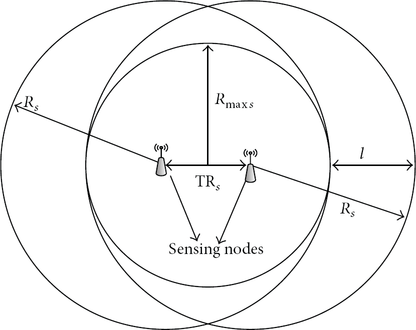
Threshold Sensing Range (
Table 1 shows all the symbols and their meanings used in this paper.
6. Relation between Number of Nodes, Grids, and Cluster Heads in the Network
In DUCA, to get the desired number of CHs, the network is divided into the same number of virtual grids. In this section we will explore the relation between
It was seen during the implementation of our proposed algorithm that for a small value of
In a network with n uniformly deployed nodes, let 

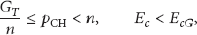
Upper limit of
The above equation can be explained as follows. For n number of nodes within a finite size of area, we should not have more than
7. Evaluation of Proposed Solution
To analyze and compare DUCA solution with the existing protocols we developed a model of WSN with randomly deployed nodes, in which DUCA was compared with the following:
LEACH protocol: as an example of dynamic cluster based protocol; grid-cluster based protocol: as an example of existing distributed uniformly cluster formation protocol; LEACH-C protocol: as an example of centrally controlled uniform cluster formation protocol.
Our aim is to show that our proposed mechanism gives a better solution, in terms of cluster sizes and distributions, compared to LEACH protocol while giving a substantial decrease of network energy consumption compared to grid-cluster and LEACH-C protocols.
7.1. Simulation Parameters
Simulation models were set up using MATLAB for LEACH, LEACH-C, grid-cluster based, and DUCA protocols. Multiple numbers of nodes ranging from 50 to 500 were considered in different field area sizes. The protocols were compared based on different parameters like network energy consumptions, cluster sizes, locations of CHs, and frame sizes. Random function seeds used for the deployment of nodes were kept the same for the four protocols, in each scenario. The CH election criteria and the nodes association criteria used in the simulations are discussed in detail in Section 4.2. Equations used for the calculation of grid ID of each node is given in Section 4.2.1. The data were collected after extensive repetitions of each simulated scenario with different random seeds.
The basic parameters used in the simulations are shown in Table 2. However, the values of m (number of frames sent per round) were not considered according to the method used in LEACH protocol. The authors of LEACH have acquired a method to establish the value of m by making it dependent on the initial energy 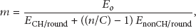
Parameters and their values used in simulations.

This is because the authors of LEACH have assumed that on average if there are 
Now for the calculation of
According to our inference the number of frames per round should be dependent on the application requirement and amount of data to be transferred in each round and not on the initial energy assigned to each node. Since in our analysis we have considered network energy consumptions and not the energy consumed in each node, therefore varying the sizes of m had no effect on overall comparison of the four protocols. Hence, for our simulations we have selected
7.2. Calculation of Distortion Percentages in Received Data
The size of a cluster can affect the data aggregation process on a CH. This can be understood through two important factors, that is, the percentage of distortions
The sizes of clusters affect the requirement of payload size at a CH. If the data collected at CH are aggregated without summarizing or compressing it then it is called packet merging. In packet merging the payload size requirement increases linearly with the increase of cluster size. Consider an example of packet merging, where each data element takes only 2 bytes and each node's ID takes 1 byte. Even with this minimal requirement of bytes, a cluster of 8 nodes requires 24 bytes in a packet, excluding header, while a cluster of 40 nodes would require 120 bytes excluding the header. On the other hand, if compression or summary (average, sum, difference, or maximum) of all readings is taken then the distortion in the individual received data increases with the increased size of clusters.
Many of the previously proposed protocols have used summary based aggregations in their networks. In summary based aggregations it has been assumed that the sensors are highly correlated. High correlation in sensors means that the sensors’ data values are close enough so that their summarized value can give an adequate overview of all of the data. However, this might not be true in real world environments. Therefore, aggregating by taking summary of multiple data values can give distortions in individual reconstructed data at the receiver.
To analyse this we have used different types of sensor data planes to collect the data through the clustered network. These data planes were synthesized by taking actual readings from IRIS motes using MTS420 sensor boards. These sensor boards give different types of sensed data readings, such as temperature, seismic vibrations, light, and humidity. Table 3 shows few of the samples of data collected from MTS420 sensor boards. There are different ranges in which these data types lie. Some of them may give high variations from one node to another or may not give variations at all. Therefore, we have used two types of sensed data planes: one with low variations of data (LV plane) and one with high variations of data (HV plane), shown in Figures 6 and 7, respectively. Also different ranges of data in each plane were considered. First, we did the summary based aggregations using these synthetic sensed data planes in a cluster based WSN. Then, the percentage of distortion
MTS420CA Sensor Board Data Readings.


Low variation data (LV) plane.

High variation data (HV) plane.
In a cluster of N nodes, if the sensed data from node j is 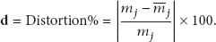
7.3. Results and Findings
In this work, we have compared the cost of clustering using single-hop communication of nodes between LEACH, LEACH-C, grid-cluster, and DUCA protocols. We have also examined the effect of cluster size on
Figure 8 gives a generalized overview of

Distortion percentage
In a network with 9% CH, there is a higher chance of 11% nodes per cluster, as shown in Figure 9, whereas the minimum energy consumed is in the range of 4 to 10% CHs in the network, as can be seen from Figure 10. Although taking higher values of CH% can give smaller clusters, the results have shown that the energy consumption increases in the network.

The probability distributions of cluster size in LEACH, LEACH-C, grid-cluster, and DUCA protocols.

Network energy consumption in 1000 rounds comparisons of LEACH, LEACH-C, grid-cluster based, and DUCA.
Concluding above paragraphs and by examining Figures 8, 9, and 10 together it can be said that around 9% CH selections can give the optimum results in terms of minimum energy consumption and distortion percentages in the data.
The results have shown that there is a significant improvement in the cluster size variations in DUCA as compared to LEACH protocol. On the other hand, the energy consumptions, in DUCA, are very low compared to the existing grid-cluster based and LEACH-C protocols.
Figure 9 shows high variations in the cluster sizes of LEACH protocol, which has been reduced significantly by implementing DUCA based CH selections. For example, in a network of 100 nodes and 4% CHs, the sizes of clusters in the case of LEACH have an average of 24 nodes with a standard deviation of 11.87 and the largest size of cluster is of 77 nodes. In the case of DUCA, these values reduced to 24 nodes, StDev = 6.47, and 50 nodes, respectively. That is, there is almost 2 times decrease in the variations of the cluster sizes. Although the cluster sizes improve significantly in LEACH-C and grid-cluster protocols, from Figure 10 it can be seen that this stability of cluster sizes costs almost 1.5 times more energy consumptions in the network.
The comparison of energy consumption within the network is shown in Figure 10. In grid-cluster based network, large amount of energy is consumed at 5% to 8% CH. According to our analysis, this is due to the fact that the selection of CHs is not done with respect to the whole network; rather, it is based on the energy levels of nodes within their respective grids only. Another reason is that the grids are considered as clusters irrespective of the distance of each node to its nearest CH, whereas in the proposed algorithm the CH selection criteria are based on the node's energy levels with respect to its grid as well as the whole network. Also, the clusters are formed on the basis of nodes’ distances to their nearest CHs. In LEACH-C, since each node needs to transmit its status to the sink in the start-up phase of each round, therefore it is more energy intensive. This cost of energy is always added up to the cost of normal data communications of the nodes.
Significant amount of energy can further be conserved if the sensing ranges of nodes are kept large enough such that the number of active nodes per cluster can be reduced. This can be implemented if a reasonable value of
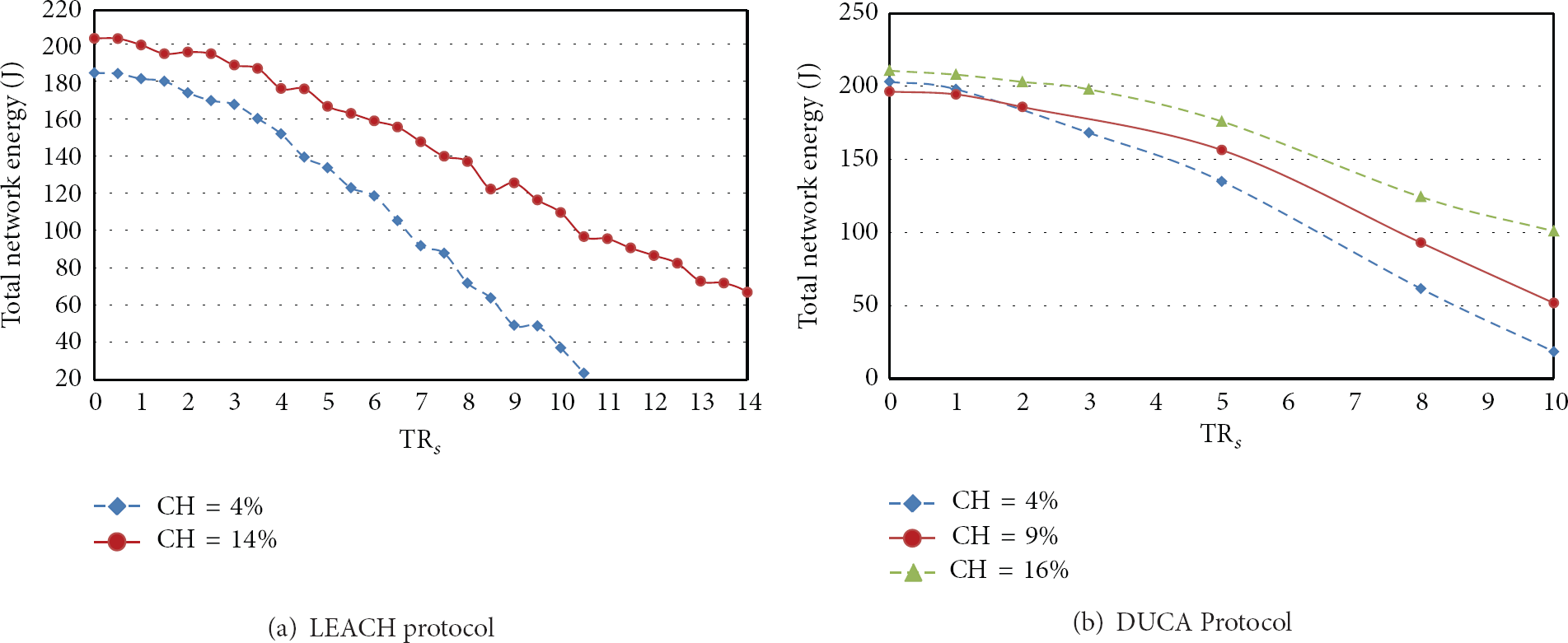
Network energy consumed in 1000 rounds; area = 1000 m2 for different

PMF comparison of cluster sizes with
Figure 13 gives the minimum network energy consumptions for different number of nodes in LEACH, LEACH-C, grid-cluster, and DUCA protocols. The effect of increase in number of nodes is much more in LEACH-C and grid-cluster protocols as compared to LEACH and DUCA, such that for 4 times increase in number of nodes the energy consumption increased to 8 times in grid-cluster and LEACH-C, while it increases 4 and 5.5 times in LEACH and DUCA, respectively. Therefore, in grid-cluster and LEACH-C based protocols the ratio of number of nodes to network energy increases from 2.7 to 5.6 approximately. In case of LEACH it remains almost the same while increases slightly from 1.9 to 2.7 in the case of DUCA.
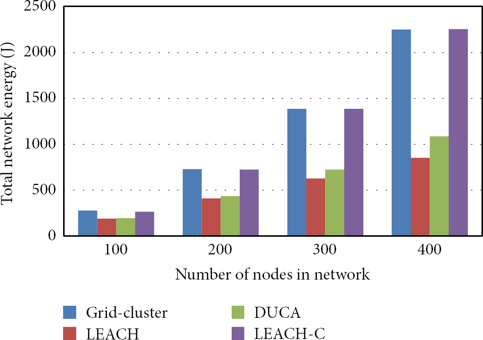
Minimum network energy consumption for different number of nodes.
8. Conclusion
In dynamic cluster based WSN, usually the sizes of clusters get highly variable when the CH selections are not based on the location of the nodes. This requires large or variable sized packets for the fusion or aggregation of data. On the other hand, if the CH selections are based only on their location, sizes of clusters become stable but it increases the overall energy consumption of the network. Centrally controlled CH selection mechanisms also give a homogeneous distribution of clusters but these procedures require extra communication energy at the start of each round. In the proposed algorithm (DUCA), cluster size variations have been substantially reduced without spending extra energy in the network. In DUCA, virtual-grid parameters have been used for even distribution of CHs while the clusters are formed on the basis of distances to CHs and not the grids. Since smaller clusters produce fewer distortions in aggregated data, the sizes of clusters are also reduced by exploiting the sensing ranges of nodes.
Footnotes
Conflict of Interests
The authors declare that there is no conflict of interests regarding the publication of this paper.