Sage Journals: Discover world-class research

Abstract

Pressure fluctuations are very important characteristics in pump turbine's operation. Many researches have focused on the characteristics (amplitude and frequencies) of pressure fluctuations at specific locations, but little researches mentioned the distribution of pressure fluctuations in a pump turbine. In this paper, 3D numerical simulations using SSTk − ω turbulence model were carried out to predict the pressure fluctuations distribution in a prototype pump turbine at pump mode. Three operating points with different mass flow rates and different guide vanes’ openings were simulated. The numerical results show how pressure fluctuations at blade passing frequency (BPF) and its harmonics vary along the whole flow path direction, as well as along the circumferential direction. BPF is the first dominant frequency in vaneless space. Pressure fluctuation component at this frequency rapidly decays towards upstream (to draft tube) and downstream (to spiral casing). In contrast, pressure fluctuations component at 3BPF spreads to upstream and downstream with almost constant amplitude. Amplitude and frequencies of pressure fluctuations also vary along different circumferential locations in vaneless space. When the mass flow and guide vanes’ opening are different, the distribution of pressure fluctuations along the two directions is different basically.

1. Introduction

Pump storage power stations (PSPs) are experiencing rapid developments in recent years, in response to the increasing demand of power/frequency modulations. A number of technical problems arise in the operations of pump turbine, which is the most important hydraulic part of PSPs. Hydraulic instability of pump turbine is found as one of the most influential problems, which is mainly caused by strong pressure fluctuations [1]. This instability can affect the safe and stable operations of the units. For instance, start-up difficulties caused by hydraulic instability have been observed in Guangzhou, Shisanling, Yixing, Tianhuangping, and many other PSPs [2 –4] in China. It is very important to study the characteristics of pressure fluctuations in the units and thus search for methods to reduce them.

Many researches have indicated that the pressure fluctuations in vaneless space of the pump turbine are stronger than those in the other positions, which are mainly caused by rotor stator interaction (RSI) [5]. The RSI phenomenon may be a combination of potential flow and viscous flow [6]. As a result of potential flow, the flow in guide vanes is periodically disturbed by rotating runner blades, which is one of the main sources of pressure fluctuations extending to the spiral casing and draft tube. The characteristics of this interaction are mainly affected by parameters of vaneless gap. The viscous flow mainly causes nonuniformity of the velocity field in the spiral casing and vaneless space. It can also cause flow separations and wakes in the whole flow domain [7].

The understanding of the mechanism of RSI and the resulting pressure fluctuations has been improved through extensive studies. For example, Sinha and Katz [8] used PIV measurements to analyze the effects of blades orientations, wakes, and level of turbulence energy. More work has been done by numerical simulations and theoretical analyses. Ruchonnet et al. [9] presented a numerical simulation of the hydroacoustic part of RSI phenomenon based on a one-dimensional model. The analysis of the pressure fluctuations resulting from the rotor-stator excitation showed several RSI patterns. Nicolet et al. [10] did similar work and discussed the influence of the thickness of guide vanes and runner blades on RSI. Tanaka [11] had developed a theoretical model to determine the diametrical vibration modes in the machine. Based on the former researches, some control measures have been developed to decrease the pressure fluctuations. Arndt et al. [12] found that by increasing the vaneless gap for 1.5 to 4.5 percent, the amplitude of pressure fluctuations decreased by 50%. Kawamoto et al. [13] found that the amplitude of the pressure fluctuations was reduced by 20–30% after increasing the guide vanes height by 40%.

Most of the researches so far have focused on the characteristics (amplitudes and frequencies) of pressure fluctuations at specific locations. In order to enhance our understanding of the mechanism of RSI, it is beneficial to have detailed information of pressure fluctuation distributions with different frequencies in the flow passage [14] and circumferential directions. In this paper, 3D numerical simulations were carried out on pressure fluctuations at different positions with different flow rates and different guide vanes’ openings, in order to study the distribution of pressure fluctuations in pump mode of a prototype pump turbine along different directions. Analysis of this problem in turbine mode will be performed in future study.

2. Pump Turbine Parameters

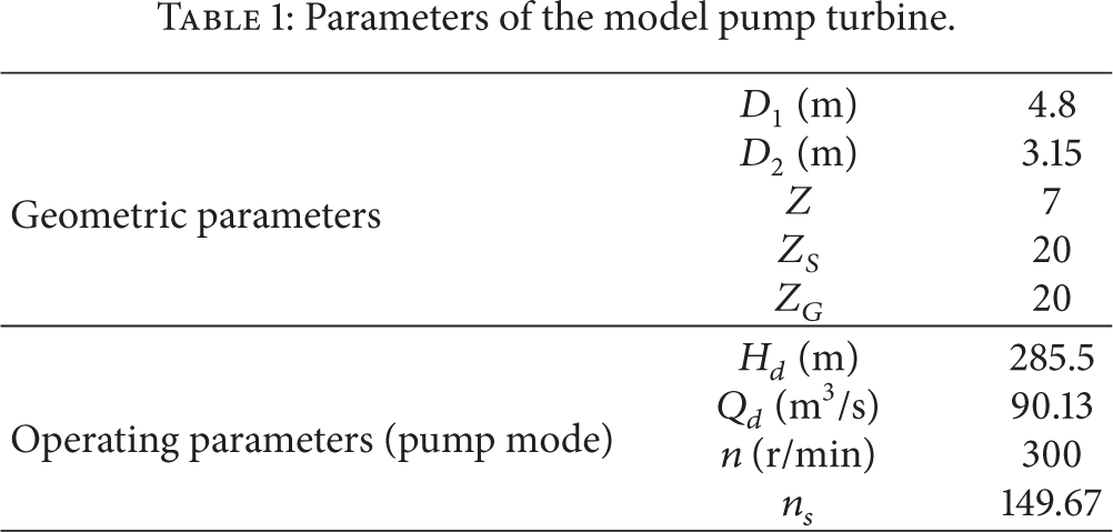
The parameters of the prototype pump turbine are shown in Table 1. D₁ and D₂ are outlet diameter and inlet diameter of the runner, respectively; Z_S, Z_G, and Z are the numbers of stay vanes, guide vanes, and runner blades, respectively; H_d is the rated head in pump mode; n is the rotational speed of the runner; Q_d is the rated discharge; n_s is the specific speed of the unit in pump mode.

Table 1:

Parameters of the model pump turbine.

Geometric parameters	D₁ (m)	4.8
	D₂ (m)	3.15
	Z	7
	Z _S	20
	Z _G	20

Operating parameters (pump mode)	H_d (m)	285.5
	Q_d (m³/s)	90.13
	n (r/min)	300
	n _s	149.67

In order to analyze the influence of guide vanes’ opening and mass flow rate, three operating points were chosen for flow simulations. The parameters of the three operating points are shown in Table 2, where α denotes the guide vanes’ opening, P denotes the input power of unit, P1 and P2 are at the same α but with different flow rates, and P2 and P3 are in the same flow rate but with different α.

Table 2:

Different operating points.

No.	α (°)	H_d (m)	Q_d (m³/s)	P (MW)

P1	22	285.5	90.13	268.8
P2	22	294.3	72.92	242.2
P3	18	311.6	72.77	240.1

The whole geometry contains spiral casing, stay vanes, guide vanes, runner, and draft tube, as shown in Figure 1.

Figure 1:

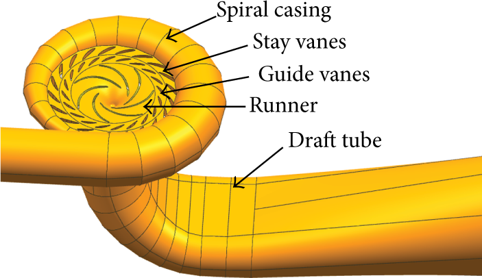
Computational domain of the prototype pump turbine.

3. Numerical Simulation Methods

3.1. Mesh Profiles

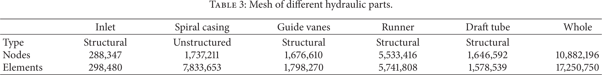
The mesh was generated by software ICEM for numerical simulations. Unstructured mesh was used in spiral casing and stay vanes, while structural mesh was used in the other parts of the hydraulic model, that is, guide vanes, runner, and draft tube. The boundary layers near stay vanes, guide vanes, and runner blades were refined to match the requirement of y⁺. The total elements number of the whole mesh was set as 17.3 million according to the mesh independence verification results shown in Figure 2, which was performed with respect to the hydraulic efficiency at one operating point. The following efficiency in this paper always denotes hydraulic efficiency of the unit. Figure 3 shows the mesh of several parts. Table 3 shows the mesh details in different parts of the model.

Table 3:

Mesh of different hydraulic parts.

	Inlet	Spiral casing	Guide vanes	Runner	Draft tube	Whole

Type	Structural	Unstructured	Structural	Structural	Structural
Nodes	288,347	1,737,211	1,676,610	5,533,416	1,646,592	10,882,196
Elements	298,480	7,833,653	1,798,270	5,741,808	1,578,539	17,250,750

Figure 2:

Mesh independence verification with respect to hydraulic efficiency.

Figure 3:

Mesh of different hydraulic parts.

3.2. Distribution of Pressure Monitoring Sensors

Pressure monitoring sensors were positioned along two directions in the pump turbine. There were 20 equally distributed sensors along the circumferential direction in the vaneless space (HVS1-20). Several other pressure sensors were placed along a flow path, that is, HC (in the spiral casing), HST2 and HST1 (in the stay vanes in different radius), HG (in the guide vanes), HFS (at the incircle of guide vanes), HVS (in the vaneless space), HD2 (in the draft tube cone), and HD6 (in the draft tube bend). The pressure sensors are shown in Figures 4 and 5.

Figure 4:

Pressure monitoring sensors in circumferential direction in vaneless space.

Figure 5:

Pressure monitoring sensors along a flow path.

3.3. Simulation Conditions

Commercial CFD code FLUENT was used to perform the simulations. SST k − ω turbulence model was chosen in the simulations. As we know, the 3D URANS methods have been used for simulating flows in complex fluid machinery because of their acceptable accuracy and low requirement for computing resources compared with LES, especially in prototype pump turbine simulation with larger geometrical scale. Comparing with other RANS turbulence models, SST k − ω model has a relatively good behavior in predicting pressure gradients and separating flow. SST k − ω model does slightly overestimate the turbulence levels in regions with large normal strain, for example, stagnation regions and regions with strong accelerations. The use of a k − ω formulation in the inner parts of the boundary layer makes the model directly usable all the way down to the wall through the viscous sublayer; hence the SST k − ω model can be used as a Low-Re turbulence model without any extra damping functions. The SST formulation also switches to a k − ε behaviour in the free-stream and thereby avoids the common k − ω problem that the model is too sensitive to the inlet free-stream turbulence properties.

Velocity inlet at the draft tube and pressure outlet in the spiral casing were set as boundary conditions of the pump turbine in the pump mode. The pressure velocity coupling was SIMPLEC scheme. The discretization was set as second-order upwind. The unsteady time step in this simulation was chosen as the time of runner rotating by 1°. The rotational speed of runner was always 300 r/min, based on which the time step was chosen as 5.56 × 10⁻⁴ seconds.

4. Results and Discussions

4.1. Accuracy of Simulation

The steady and unsteady simulation results were compared to the experimental results to validate the accuracy of the numerical simulations. The experiments were carried out by the manufacturers for acceptance tests of the prototype pump turbine.

Figure 6 shows the comparison results. The head and efficiency are almost the same as the experimental data, which proved the accuracy of the simulations.

Figure 6:

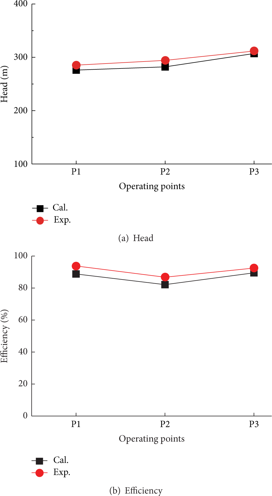
Accuracy validation of numerical simulations.

Comparisons between simulation results and experimental results were also performed to validate the accuracy of unsteady simulation results on pressure fluctuations. The results of relative amplitude (defined as Δp/ρgH, where Δp is the total amplitude of pressure fluctuations, ρ is the density of water, and H is the hydraulic head) in Table 4 and frequency spectrum in Figure 7 indicate that the accuracy of numerical calculations is acceptable. The blade passing frequency (BPF) in this case is 35 Hz (rotating speed of the runner is 300 r/min and the number of blades is 7).

Table 4:

Comparison of relative pressure fluctuation amplitudes between simulations and experiments.

	HC	HVS	HD2

Exp.	1.59%	4.42%	0.81%
Cal.	1.68%	5.24%	0.85%

Figure 7:

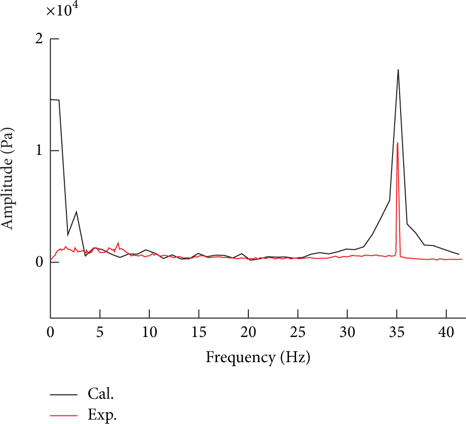
Comparison of pressure fluctuations spectrum between simulations and experiments in vaneless space.

4.2. Distribution in Circumferential Direction

The pressure fluctuations at different positions in vaneless space at P1 (best efficiency point in pump mode) are shown in Figure 8. The point with the highest relative amplitude occurs at position HVS16, which is very close to the position of the longest stay vane (Figure 4).

Figure 8:

Relative pressure fluctuations amplitude in vaneless space (P1).

The frequency spectrum at different positions along vaneless space is shown in Figure 9, from which it can be concluded that the pressure fluctuations of BPF and its multiple frequencies are the main dominant frequencies in vaneless space. The BPF is the first dominant frequency, and its amplitude varies along different positions in vaneless space. The 3BPF is the second dominant frequency, and its amplitude keeps almost constant with varying positions. A more detailed result can be seen from Figure 10.

Figure 9:

Frequency spectrum of pressure fluctuations at different positions in vaneless space (P1).

Figure 10:

Distribution of pressure fluctuations components of BPF, 2BPF, and 3BPF at different positions in vaneless space (P1).

Figure 10 shows the distribution of pressure fluctuation components of BPF, 2BPF, and 3BPF along different positions in vaneless space. The components of BPF and 2BPF have similar distributions, reaching the highest values at the point HVS16. The distribution trend of relative amplitude in Figure 8 is similar to BPF component since BPF is the first dominant frequency in vaneless space. The component of 3BPF has a different distribution, almost keeping the constant amplitude along the circumferential direction. Component of 3BPF is an expected frequency based on the interaction between 7 runner blades and 20 guide vanes [15]. The difference between BPF and 3BPF distributions indicates that components of these two frequencies may transfer in different modes because of their different sources. BPF is mainly caused by rotor part in RSI, while 3BPF is mainly caused by stator part in RSI.

4.3. Distribution in Flow Path Direction

Figure 11(a) shows the relative amplitude analysis of pressure fluctuations along a flow path. Pressure fluctuations reach the highest value at HVS, HFS, and HG. Figure 11(b) shows different frequency spectra at different positions. The amplitudes of BPF and 2BPF at HVS, HFS, and HG are relatively large but decrease rapidly to a small value at spiral casing and draft tube. The variation of the amplitudes of 3BPF at different positions along the flow path is smaller than that of BPF. Detailed distributions of amplitudes of BPF, 2BPF, and 3BPF can be seen from Figure 12. BPF is the first dominant frequency close to the vaneless space, and its amplitude decreases rapidly at the spiral casing and draft tube. On the other hand, 3BPF spreads highlighting from vaneless space to upstream and downstream with small change in amplitude. Component of 3BPF is larger than BPF at spiral casing and draft tube, while component of BPF is the largest at vaneless zone.

Figure 11:

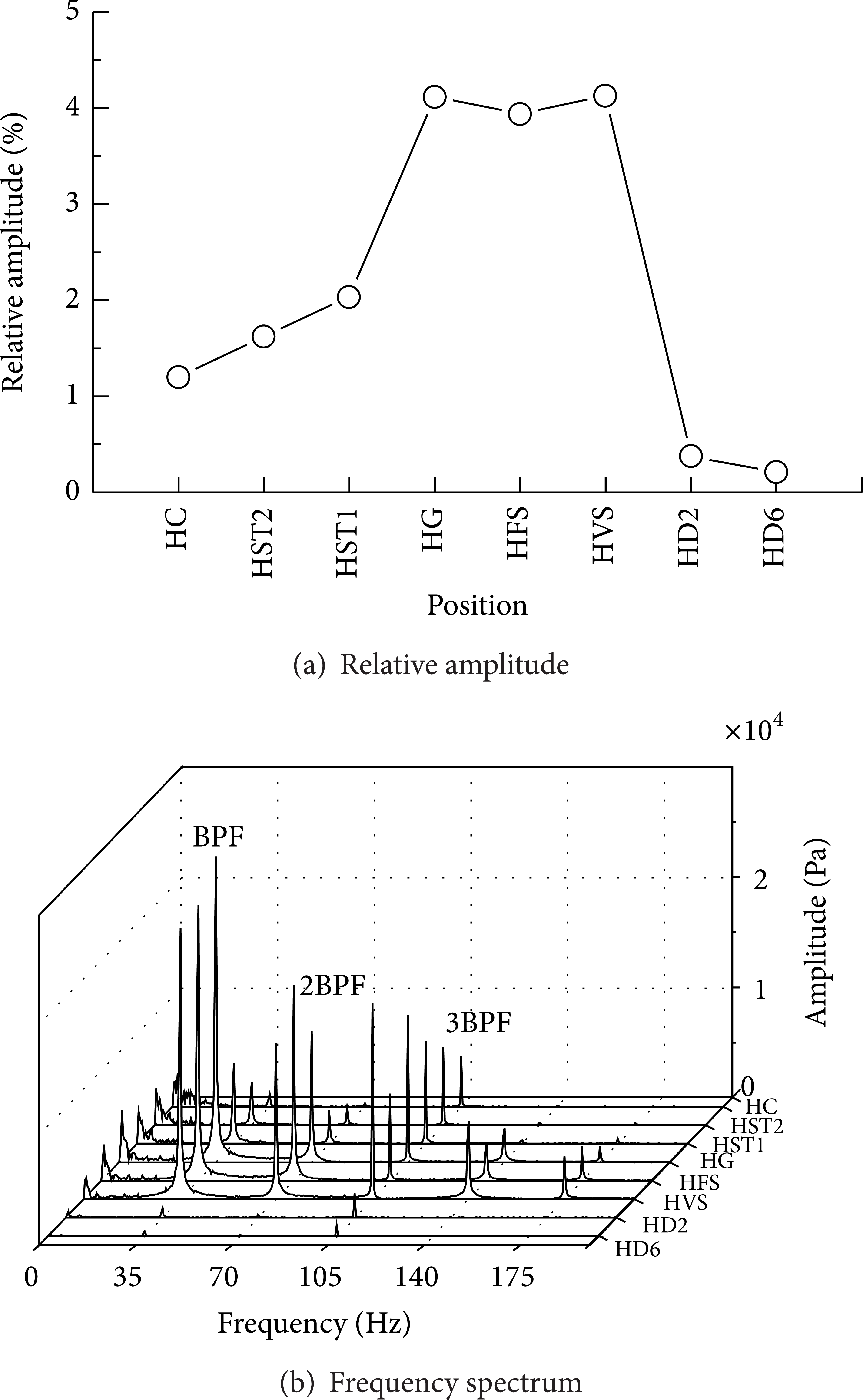
Relative amplitude and frequency spectrum of pressure fluctuations at different positions along a flow path (P1).

Figure 12:

Distribution of pressure fluctuations components of BPF, 2BPF, and 3BPF at different positions along a flow path (P1).

4.4. Influence of Mass Flow Rate

In order to analyze the influence of the mass flow rate on the distribution of pressure fluctuations, another operating point (P2) with a different flow rate is compared below. Other parameters including guide vanes’ opening of P2 are the same as P1, while the flow rate of P2 is 20% smaller than that of P1.

Figure 13(a) shows the relative amplitude of pressure fluctuations in vaneless space at P1 and P2. It is obvious that the pressure fluctuations become the strongest at position HVS16 in P1 and P2. The general distribution is similar between P1 and P2 but the relative amplitude of P2 is larger than that of P1, because P1 is the best efficiency point. Relative amplitude reaches a higher value at HVS18 in P2 because component of low frequency is very high at HVS18, which can be seen from Figure 13(b).

Figure 13:

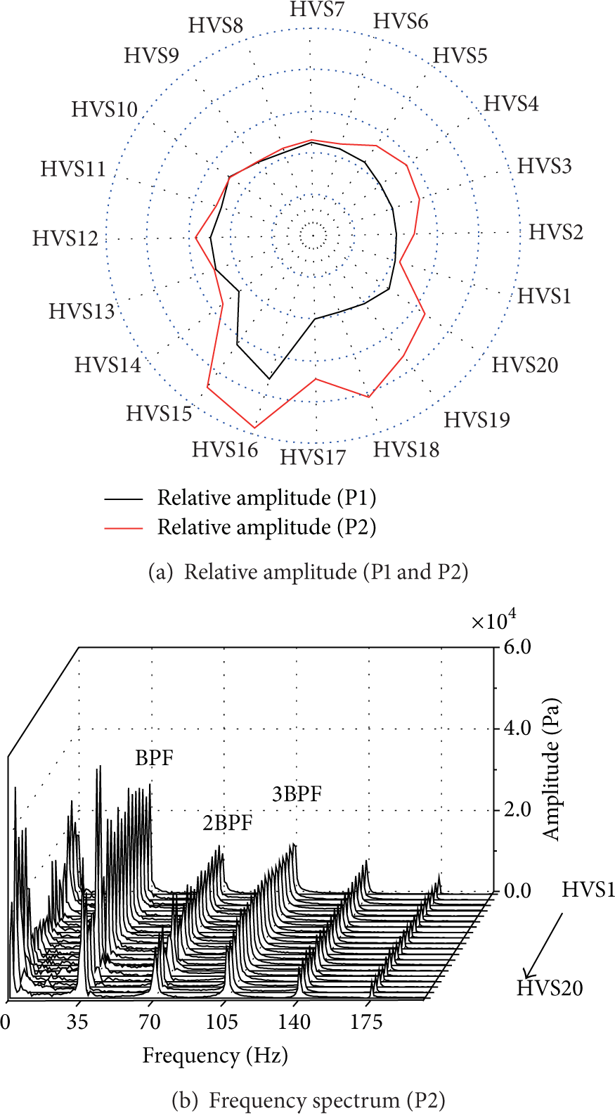
Relative amplitude and frequency spectrum of pressure fluctuations in vaneless space with different flow rates.

Figure 14 shows the distribution comparison of pressure fluctuations components of BPF, 2BPF, and 3BPF in vaneless space at P1 and P2. The general distributions of BPF, 2BPF, and 3BPF are similar. Component of BPF in P2 is larger than that in P1, while component of 3BPF in P2 is smaller than that in P1. This indicates that decreasing flow rate strengthens BPF, while it weakens 3BPF.

Figure 14:

Distribution of pressure fluctuations components of BPF, 2BPF, and 3BPF at different positions in vaneless space with different flow rates (P1 and P2).

Figure 15(a) shows the relative amplitude of pressure fluctuations at different positions along a flow path at P1 and P2. The relative amplitude in P1 reaches the highest value at HVS, while in P2 it reaches the highest value at HG (in the middle of guide vanes channel). It can be seen from Figure 15(b) that the low frequency replaces the BPF to be the first dominant frequency at HG. Pressure fluctuations with low frequency at HVS, HFS, HST1, and HST2 also have relatively large amplitude. The low frequency occurs when the unit is not operating at the best efficiency point. Figure 16 shows the distribution difference of pressure fluctuations components of BPF, 2BPF, and 3BPF at P1 and P2. With decreasing flow rate, BPF becomes higher close to vaneless space, while it becomes lower far away from vaneless space. 2BPF keeps the same and 3BPF becomes lower along a whole flow path with decreasing flow rate.

Figure 15:

Relative amplitude and frequency spectrum of pressure fluctuations at different positions along a flow path with different flow rates.

Figure 16:

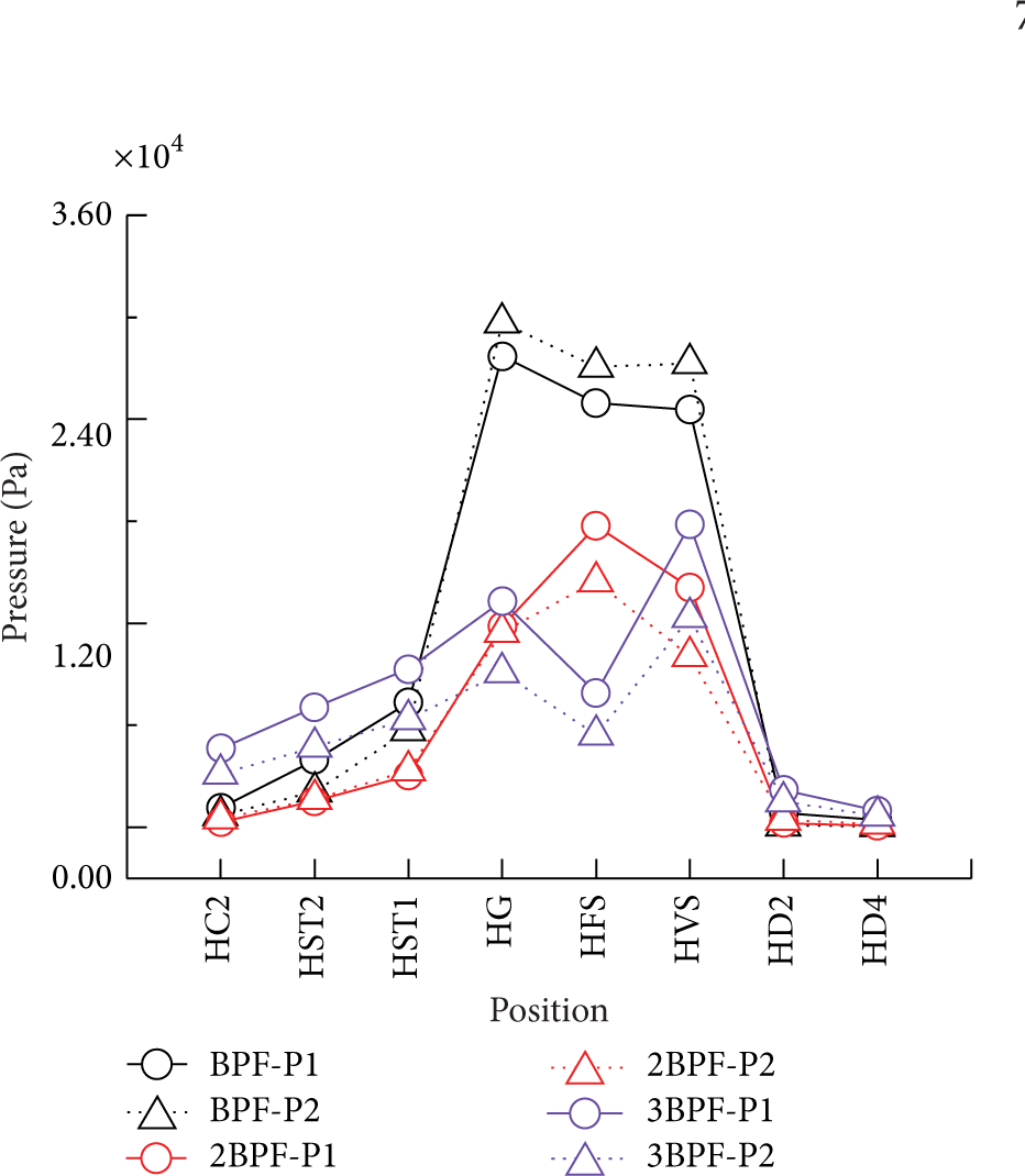
Distribution of pressure fluctuations components of BPF, 2BPF, and 3BPF at different positions along a flow path (P1 and P2).

4.5. Influence of Guide Vanes’ Opening

In order to analyze the influence of guide vanes’ opening on the distribution of pressure fluctuations, another operating point (P3) with a different guide vanes’ opening is compared below. Other parameters including flow rate of P3 are the same with P2, while the guide vanes’ opening of P3 is 18° (22° at P2). Conclusion can be drawn from Figure 6(b) that efficiency of P3 is higher than that of P2. The guide vanes’ opening of P2 is the same as the best efficiency point P1 but the flow rate is lower, while the guide vanes’ opening of P3 is smaller than P1 and flow rate is also smaller. That is why the efficiency of P3 is higher than P2.

Figure 17(a) shows the relative amplitude of pressure fluctuations in vaneless space at P2 and P3. Pressure fluctuations reach the highest amplitudes at HVS15 in P3 and at HVS16 in P2. The general distribution is similar between P2 and P3 but the relative amplitude of P2 is larger than that of P3. The low frequency is much smaller at P3 than at P2, which can be seen from the comparison between Figures 17(b) and 13(b).

Figure 17:

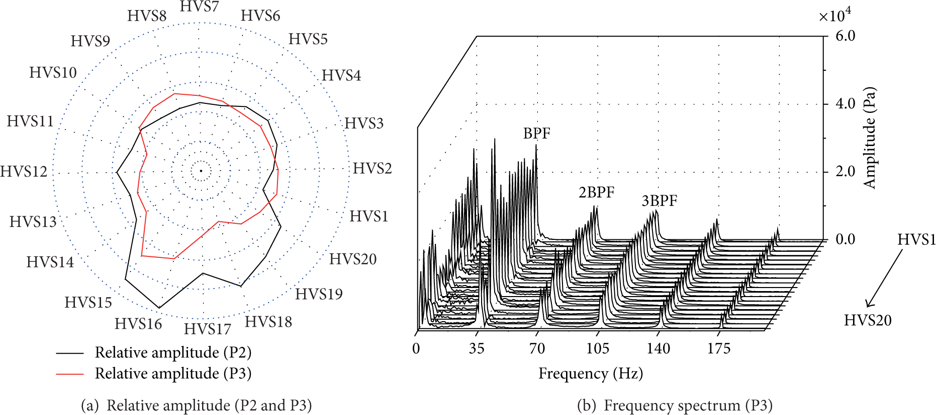
Relative amplitude and frequency spectrum of pressure fluctuations in vaneless space with different guide vanes’ openings.

Figure 18 shows the distribution comparison of pressure fluctuations components of BPF, 2BPF, and 3BPF in vaneless space at P2 and P3. The general distributions of BPF, 2BPF, and 3BPF are similar. Components of BPF and 2BPF are similar at P2 and P3, while component of 3BPF at P2 is larger than that at P3. That means that increasing guide vanes’ opening only influences the component of 3BPF by strengthening its amplitude. The components of BPF and 2BPF remain almost unchanged with changing guide vanes’ opening.

Figure 18:

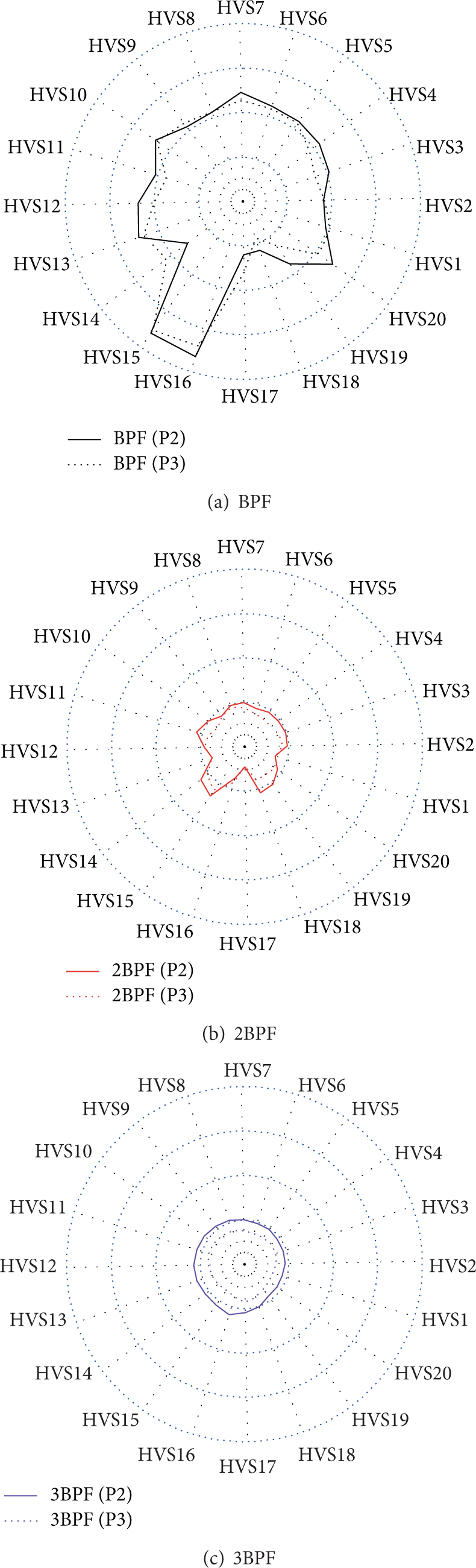
Distribution of pressure fluctuations components of BPF, 2BPF, and 3BPF at different positions in vaneless space with different guide vanes’ openings (P2 and P3).

Figure 19(a) shows the relative amplitude of pressure fluctuations at different positions along a flow path at P2 and P3. The relative amplitude at P2 and P3 reaches the highest value at HG (in the middle of the flow channel between guide vanes) because the low frequency replaces the BPF to be the first dominant frequency at HG. Pressure fluctuations with low frequency at HVS, HFS, HST1, and HST2 also have relatively large amplitudes. The relative amplitude of pressure fluctuations at vaneless zone at P2 is larger than that at P3, while at the other zone the amplitude is almost the same. Figure 20 shows the distribution difference of pressure fluctuations components of BPF, 2BPF, and 3BPF at P2 and P3. With increasing guide vanes’ opening, the components of BPF and 2BPF remain the same along the whole flow path. Component of 3BPF increases along the whole flow path with increasing guide vanes’ opening.

Figure 19:

Relative amplitude and frequency spectrum of pressure fluctuations at different positions along a flow path with different guide vanes’ openings.

Figure 20:

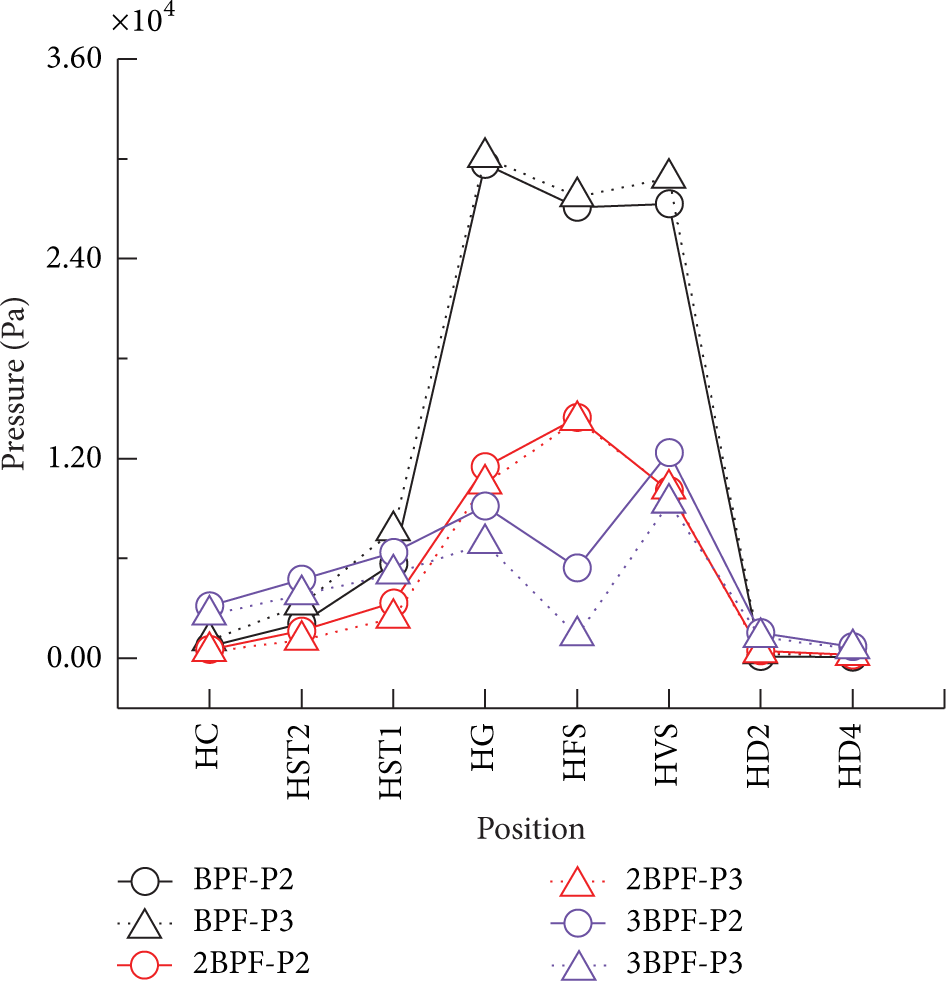
Distribution of pressure fluctuations components of BPF, 2BPF, and 3BPF at different positions along a flow path with different guide vanes’ openings (P2 and P3).

5. Conclusions

3D numerical simulations using SST k − ω turbulence model were performed in this paper to analyze the distribution of pressure fluctuations in prototype pump turbine at pump mode. Influences of flow rate and guide vanes’ opening were taken into account to show the distribution of pressure fluctuations in both circumferential and flow path directions. The conclusions can be drawn as follows. The highest pressure fluctuations along the circumferential direction occur at positions that are close to the volute tongue. Components of BPF and 2BPF also reach the highest value the same position, while component of 3BPF keeps almost constant along circumferential direction. The highest pressure fluctuations occur in vaneless space along a flow path direction. Component of BPF is high in vaneless space but rapidly decays towards upstream (to draft tube) and downstream (to spiral casing). However, pressure fluctuations component of 3BPF spreads to upstream and downstream with almost constant amplitudes. This indicates that the component of 3BPF varies slightly in the whole unit.

With different flow rates and guide vanes’ openings, the distribution of pressure fluctuations along circumferential and flow path direction is similar to the original operating point except some variations. Component of low frequency increases when the pump turbine is not operating at the best efficiency point. With decreasing flow rate, component of BPF increases in vaneless space but decreases away from vaneless space, while component of 3BPF decreases within the whole unit. With increasing guide vanes’ opening, distribution of BPF and 2BPF varies slightly, while component of 3BPF increases along the whole unit.

In this study, the two most important frequencies (BPF and 3BPF) caused by RSI in the studied prototype pump turbine show totally different distributions along circumferential direction and flow path direction. This indicates that different components of RSI (different interaction mode) may have different performances in the pump turbine unit, which should draw more attention in future investigations.

Conflict of Interests

The authors declare that there is no conflict of interests regarding the publication of this paper.

Footnotes

Acknowledgments

The authors would like to thank the National Natural Science Foundation of China (no. 51076077) and the National Science and Technology Ministry of China (ID: 2008BAC48B02) for their financial supports.

References

Nennemann

T. C.

, and Farhat

, “CFD prediction of unsteady wicket gate-runner interaction in Francis turbines: a new standard hydraulic design procedure,” in Proceedings of the 14th Waterpower, Austin, Tex, USA, 2005.

M. Y.

, “Technical performance analysis and comparison of pump turbine in Guangzhou PSPs and Shisanling PSP,” Dong fang Electrical Machine, vol. 3, pp. 66–72, 1995.

Nennemann

and Parkinson

, “YiXing pump turbine guide vane vibrations: problem resolution with advanced CFD analysis,” in Proceedings of the 25th IAHR Symposium on Hydraulic Machinery and Systems, 2010.

S. R.

, “Analysis of vibration in Tianhuangping PSP station,” Mechanical and Electrical Technique of Hydropower Station, vol. 1, pp. 1–9, 1999.

Parrondo-Gayo

J. L.

González-Pérez

, and Fernández-Francos

, “The effect of the operating point on the pressure fluctuations at the blade passage frequency in the volute of a centrifugal pump,” Transactions of the ASME Journal of Fluids Engineering, vol. 124, no. 3, pp. 784–790, 2002.

Dring

R. P.

Joslyn

H. D.

Hardin

L. W.

, and Wagner

J. H.

, “Turbine rotor-stator interaction,” ASME Journal of Engineering for Powe, vol. 104, no. 4, pp. 729–742, 1982.

Zobeiri

, Investigations of time dependent flow phenomena in a turbine and a pump-turbine of Francis type: rotor-stator interactions and precessing vortex rope [EPFL Doctoral Thesis], 2009, No. 4272.

Sinha

and Katz

, “Quantitative visualization of the flow in a centrifugal pump with diffuser vanes—I: on flow structures and turbulence,” Journal of Fluids Engineering, vol. 122, no. 1, pp. 97–107, 2000.

Ruchonnet

Nicolet

, and Avellan

, “Hydroacoustic modeling of rotor stator interaction in francis pump-turbine,” in Proceedings of the IAHR International Meeting of WG on Cavitation and Dynamic Problems in Hydraulic Machinery and Systems, 2006.

10.

Nicolet

Ruchonnet

, and Avellan

, “One-dimensional modeling of rotor stator interaction in francis pump-turbine,” in Proceedings of the 23rd IAHR Symposium on Hydraulic Machinery and Systems, 2006.

11.

Tanaka

, “Vibration behavior and dynamic stress of runners of very high head reversible pump turbine,” International Journal of Fluid Machinery and Systems, vol. 4, no. 2, pp. 289–306, 2011.

12.

Arndt

Acosta

A. J.

Brennen

C. E.

, and Caughey

T. K.

, “Experimental investigation of rotor-stator interaction in a centrifugal pump with several vaned diffusers,” Journal of Turbomachinery, vol. 112, no. 1, pp. 98–108, 1990.

13.

Kawamoto

Niikura

Satoh

Harada

, and Terasaki

, “Reduction of stress amplitude in the runner of ultrahigh head pump turbines,” Transactions of the Japan Society of Mechanical Engineers B, vol. 59, no. 558, pp. 481–486, 1993.

14.