Study on a New Steering Mechanism for Point-the-Bit Rotary Steerable System

Abstract

This paper presents a novel steering mechanism embedded in a point-the-bit rotary steerable system (RSS) for oilfield exploitation. The new steering mechanism adopts a set of universal joints to alleviate the high alternative strain on drilling mandrel and employs a specially designed planetary gear small tooth number difference (PGSTD) to achieve directional steering. Its principle and characteristics are explained and examined through a series of analyses. First, the eccentric displacement vector of the offset point on the drilling mandrel is formulated and kinematic solutions are established. Next, structural design for the new steering mechanism is addressed. Then, procedures and program architectures for simulating offset state of the drilling mandrel and motion trajectory of the whole steering mechanism are presented. After that, steering motion simulations of the new steering mechanism for both 2D and 3D well trajectories are then performed by combining LabVIEW and SolidWorks. Finally, experiments on the steering motion control of the new steering mechanism prototype are carried out. The simulations and experiments reveal that the steering performance of the new steering mechanism is satisfied. The research can provide good guidance for further research and engineering application of the point-the-bit RSS.

1. Introduction

Directional drilling is crucial for oilfield exploration and development. The introduction of rotary steerable system (RSS) in the late 1990s marked a significant advance in drilling technology. RSSs are complex drilling tools integrated with mechanical, electrical, and hydraulic components [1]. Compared with traditional drilling tools, the advantages of RSS technology include real-time drilling direction adjustment, intelligent well trajectory control, and smooth well trajectory without spiral borehole [2–5]. A rotary steerable system mainly consists of steering mechanism, a measurements-while-drilling system (MWD), a ground-to-underground two-way communication system, and a ground monitoring system [6, 7]. Among these components, the steering mechanism is crucial. With the steering control of the steering mechanism, the drilling direction of the drill bit can be changed continuously during drilling [6–8].

According to the steering control principle, existing steering mechanisms can be classified into two types, namely, push-the-bit type and point-the-bit type [9]. For most early RSSs, the steering mechanisms belong to push-the-bit type, like the PowerDrive RSS from Schlumberger and the AutoTrack RSS from Baker Hughes. The steering mechanisms of push-the-bit type are normally powered by hydraulic and mainly consisted of an outer cylinder, hydraulic distribution components, control components, and drilling mandrel. On the outer cylinder, three stretching pads are placed uniformly and each stretching pad is connected to a hydraulic cylinder. During drilling process, the stretching pads will contact with the well wall in turn powered by hydraulic cylinders. Due to reacting force, the drilling mandrel will be deviated from its present pointing axis and the drilling direction will be changed [10–12]. Although the push-the-bit steering mechanism can achieve flexible directional steering, several problems are observed in practice. A major problem is that the intensive impact on the stretching pads may cause violent vibrations of the steering mechanism and lead to poor drilling well holes. Additionally, it is difficult to seal the hydraulic-powered steering mechanism [13].

RSSs with point-the-bit steering mechanism, for example, the Geo-Pilot RSS from Halliburton and the PowerDrive Xceed RSS from Schlumberger, were proposed later to overcome the above drawbacks [14]. The point-the-bit steering mechanism normally utilizes a set of offset mechanisms to deflect the drilling mandrel and hence change the drilling direction. The offset mechanism consisted of several eccentric rings. Each eccentric ring is powered by motors and can rotate, respectively. During the rotation of the eccentric rings, the offset amplitude and offset phase of the drilling mandrel can be adjusted [15, 16]. The point-the-bit steering mechanism can afford better well holes quality, longer service life, lower vibration, and better efficiency of rock cutting. Moreover, the point-the-bit steering mechanism can control its trajectory more accurately and quicker than the push-the-bit steering mechanism, as it is powered by motors rather than hydraulic cylinders. Further, there is no trouble on sealing the steering mechanism [17]. Nevertheless, existing point-the-bit steering mechanism is not perfect, although the existing point he-bit steering mechanism has demonstrated the capbility of the existing point the-bit steering mechanism capability to steer the drill bit to target locations. A prominent problem is the high alternative strain on the drilling mandrel, which may lead to a reduced service life of the mandrel and a severe wear of the eccentric rings [17].

Considering the limitations of existing steering mechanism, the authors propose a novel steering mechanism used in point-the-bit RSSs. It is conceived that the new steering mechanism should be easier to assemble and can alleviate the high alternative strain on drilling mandrel, and additionally it can simplify the control process [15, 18]. This paper will try to investigate the characteristics of the new mechanism, and the related contents are organized as follows. Section 2 explains the working principle and the kinematic solution of the new steering mechanism. Section 3 introduces the structural design and the control system design of the new steering mechanism. Section 4 investigates the combined steering motion simulations of the new steering mechanism. Section 5 demonstrates the prototype experiments and discusses the characteristics of the proposed mechanism. And finally Section 6 draws the conclusion.

2. Working Principle and Kinematic Solution

2.1. Working Principle of the New Steering Mechanism

As shown in Figure 1, the drilling shaft is separated by the universal joints into two portions, namely, a normal drilling shaft and a hollow drilling mandrel. With the new layout, the drilling mandrel can be easily offset by offset device [19]. Moreover, the alternative strain on the drilling mandrel is expected to be much reduced, and the mechanical structure can be greatly simplified. Besides, the universal joints can compensate the displacement of the drilling mandrel along the axis direction.

Figure 1:

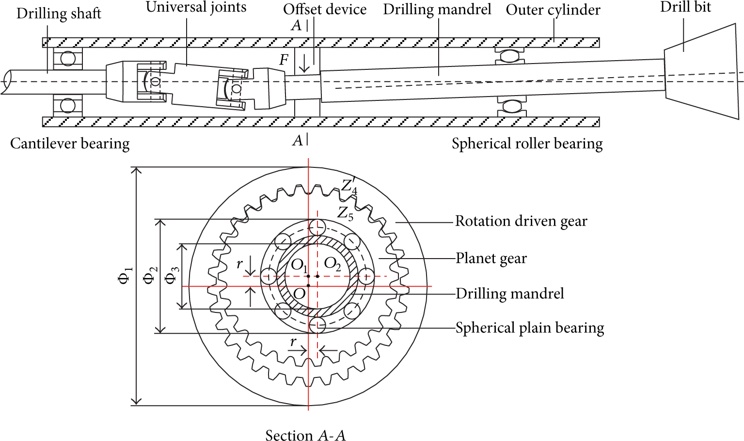
Schematic layout of the new steering mechanism.

The offset device is the key part of the new steering mechanism. It consists of a specially designed planetary gear small tooth number difference (PGSTD) and two servomotors. In the PGSTD, the revolution driven gear has an eccentric hole where the planet gear is located inside. The planet gear also has an eccentric hole where the drilling mandrel passes through. Driven by two motors, the PGSTD can continuously offset the drilling mandrel from its present pointing axis.

As illustrated in Figure 1, O, O₁, and O₂ are, respectively, the centers of gyration for rotation driven gear, planet gear, and drilling mandrel. Z₄′ and Z₅ are, respectively, the inner tooth numbers of the rotation driven gear and the tooth number of the planet gear. And Φ₁, Φ₂, and Φ₃ are the dimensional parameters of the PGSTD. Note that the distance of OO₁ and that of O₁O₂ are both denoted as r. These parameters will be specified considering the steering performance demand and the volume limitation of the new steering mechanism.

The schematic structure of offset device is further detailed in Figure 2. Two DC servomotors (M1 and M2) control the rotation and the revolution of the planet gear separately. When M1 rotates, the planet gear will rotate around its own axis. When M2 rotates, the planet gear will revolute around the axis of the steering mechanism. In the meantime, the planet gear will rotate around its own axis due to the gearing interaction between the rotation driven gear and the planet gear. As the drilling mandrel is constrained in the eccentric hole of the planet gear by a set of spherical plain bearings, it always follows the movement of the planet gear.

Figure 2:

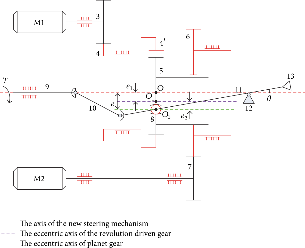
The schematic structure of the offsetting device in the steering mechanism. 1: DC servomotor M1, 2: DC servomotor M2, 3: rotation drive gear, 4: rotation driven gear, 5: planet gear, 6: revolution driven gear, 7: revolution drive gear, 8: spherical plain bearings, 9: drilling shaft, 10: universal joints, 11: drilling mandrel, 12: spherical roller bearing, 13: drill bit.

As illustrated in Figure 2, O₂ is also the offset point on the drilling mandrel. The displacement vector (e) from O to O₂ is defined as the eccentric displacement vector of the offset point on the drilling mandrel. According to vector composition principle, e is the result of vector composition by e₁ (displacement vector from O to O₁) and e₂ (displacement vector from O₁ to O₂). Obviously, e determines the steering performance of the new steering mechanism. With a suitable revolution and rotation of the planet gear, the amplitude of e ranges from 0 to 2r, and the phase ranges from 0° to 360°. A special case is shown in the figure when the directions of e₁ and e₂ are in coincidence, and hence the amplitude of e reaches the maximum.

Considering the demanded performances and the internal volume limitation of our prototype, the eccentric displacement values are defined as e₁ = e₂ = r = 5.25 mm. And then, a steering range of 1 degree is achieved. Other structural parameters of the new steering mechanism are chosen as shown in Table 1 [20].

Table 1:

Structural parameters of the new steering mechanism.

Z 3	Z 4	Z4′	Z 5	Z 6	Z 7	Modulus	Φ1 (mm)	Φ2 (mm)	Φ3 (mm)
17	38	33	30	38	17	3.5	250	100	60

2.2. Kinematic Solution for the New Steering Mechanism

2.2.1. Forward Kinematic Solution

A forward kinematic solution is used to determine the resultant eccentric displacement vector of the offset point on the drilling mandrel from the rotation angles of the two input motors. To obtain the solution, a kinematic model of the eccentric displacement vector of the offset point on the drilling mandrel is built as illustrated in Figure 3.

Figure 3:

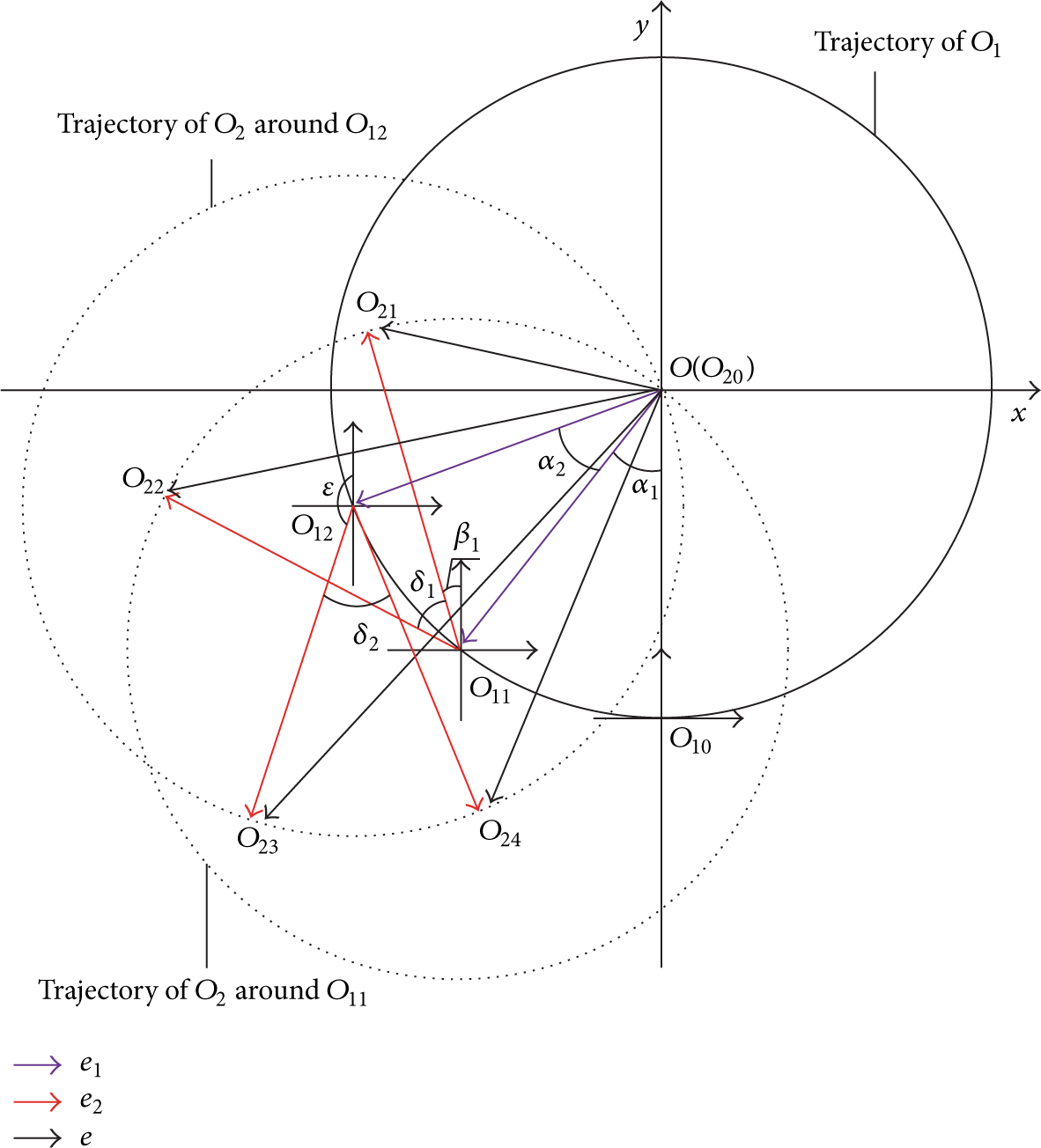
The kinematical model of the eccentric displacement vector.

Initially, the steering mechanism does not offset the drilling mandrel and the resultant eccentric displacement vector (e) of the offset point is 0. Under the condition, O₂ is located at O₂₀ which is coincident with the origin O.

Take the points O and O₁ as the origins to establish the system coordinate and the local coordinate system, respectively. And, hence, the resultant eccentric displacement vector (e) is synthesized by e₁ in the system coordinate and e₂ in the local coordinate system.

In this special PGSTD, when the planet gear revolutes, it will rotate around its own axis due to the gearing interaction. According to the drive ratio and structural parameters of the PGSTD, the relationship between the revolution angle α and the rotation angle β can be derived as

$\beta =-\mathrm{0.1}\alpha .$

(1)

During steering process, M2 firstly starts to drive the revolution of the planet gear. And then, M1 starts to drive the rotation of the planet gear to take the drilling mandrel to the target position. The process of the forward kinematic solution for the new steering mechanism is shown as follows.

When the revolution angle of the planet gear is α₁, the center of gyration for the planet gear will move from O₁₀ to O₁₁. With the effect of the gearing interaction, the rotation angle of the planet gear is β₁, leading to the offset point on the drilling mandrel moving from O₂₀ to O₂₁. In the system coordinate, e₁ (OO₁₁) can be written as

$e_1=O{O}_{11}=\left(\begin{array}{c}-r\sin {\alpha }_{\mathrm{1}}\\ -r\cos {\alpha }_{\mathrm{1}}\end{array}\right).$

(2)

In the local coordinate (take O₁₁ as the origin), e₂ (O₁₁O₂₁) can be written as

$e_2=O_{11}{O}_{21}=\left(\begin{array}{c}r\cos \left(\mathrm{9}{\mathrm{0}}^{°}+{\beta }_{\mathrm{1}}\right)\\ r\sin \left(\mathrm{9}{\mathrm{0}}^{°}+{\beta }_{\mathrm{1}}\right)\end{array}\right)=\left(\begin{array}{c}-r\sin {\beta }_{\mathrm{1}}\\ r\cos {\beta }_{\mathrm{1}}\end{array}\right).$

(3)

According to vectors synthesizing principle, the resultant eccentric displacement vector of the offset point on the drilling mandrel is

$e=O{O}_{21}=e_1+e_2=\left(\begin{array}{c}-r\sin {\alpha }_{\mathrm{1}}-r\sin {\beta }_{\mathrm{1}}\\ -r\cos {\alpha }_{\mathrm{1}}+r\cos {\beta }_{\mathrm{1}}\end{array}\right).$

(4)

When the revolution is completed, M1 starts to drive the planet gear rotating around O₁₁. When the rotation angle is δ₁, the offset point on the drilling mandrel will move from O₂₁ to O₂₂. New e₂ (O₁₁O₂₂) in the local coordinate is

$e_2=O_{11}{O}_{22}=\left(\begin{array}{c}r\cos \left({\delta }_{\mathrm{1}}+{\beta }_{\mathrm{1}}+\mathrm{9}{\mathrm{0}}^{°}\right)\\ r\sin \left({\delta }_{\mathrm{1}}+{\beta }_{\mathrm{1}}+\mathrm{9}{\mathrm{0}}^{°}\right)\end{array}\right)=\left(\begin{array}{c}-r\sin \left({\beta }_{\mathrm{1}}+{\delta }_{\mathrm{1}}\right)\\ r\cos \left({\beta }_{\mathrm{1}}+{\delta }_{\mathrm{1}}\right)\end{array}\right).$

(5)

Finally, the resultant eccentric displacement vector is

$e=O{O}_{22}=e_1+e_2=\left(\begin{array}{c}-r\sin {\alpha }_{\mathrm{1}}-r\sin \left({\beta }_{\mathrm{1}}+{\delta }_{\mathrm{1}}\right)\\ -r\cos {\alpha }_{\mathrm{1}}+r\cos \left({\beta }_{\mathrm{1}}+{\delta }_{\mathrm{1}}\right)\end{array}\right).$

(6)

Hereto, the first steering adjustment for the drilling direction has been completed. To achieve further directional steering, the steering mechanism will act in the same way. When the second revolution angle of the planet gear is α₂, the center of gyration for the planet gear will rotate around O from O₁₁ to O₁₂. In the meanwhile, the offset point on the drilling mandrel will move from O₂₂ to O₂₃. In the system coordinate, e₁ (OO₁₂) can be written as

$e_1=O{O}_{12}=\left(\begin{array}{c}-r\sin \left({\alpha }_{\mathrm{1}}+{\alpha }_{\mathrm{2}}\right)\\ -r\cos \left({\alpha }_{\mathrm{1}}+{\alpha }_{\mathrm{2}}\right)\end{array}\right).$

(7)

In the local coordinate (take O₁₂ as the origin), e₂ (O₁₂O₂₃) can be written as

$e_2=O_{12}{O}_{23}=\left(\begin{array}{c}r\cos \epsilon \\ r\sin \epsilon \end{array}\right),$

(8)

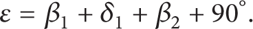
where ε is the whole rotation angle of the planet gear from the initial state and it can be expressed as

$\epsilon ={\beta }_{\mathrm{1}}+{\delta }_{\mathrm{1}}+{\beta }_{\mathrm{2}}+\mathrm{9}{\mathrm{0}}^{°}.$

(9)

And hence e₂ can be further expressed as

$e_{\mathrm{2}}=\left(\begin{array}{c}-r\sin \left({\beta }_{\mathrm{1}}+{\delta }_{\mathrm{1}}+{\beta }_{\mathrm{2}}\right)\\ r\cos \left({\beta }_{\mathrm{1}}+{\delta }_{\mathrm{1}}+{\beta }_{\mathrm{2}}\right)\end{array}\right).$

(10)

As a result, the resultant eccentric displacement vector is

$\begin{array}{l}e=O{O}_{23}=e_1+e_2\\ =\left(\begin{array}{c}-r\sin \left({\alpha }_1+{\alpha }_2\right)-r\sin \left({\beta }_1+{\delta }_1+{\beta }_2\right)\\ -r\cos \left({\alpha }_1+{\alpha }_2\right)+r\cos \left({\beta }_1+{\delta }_1+{\beta }_2\right)\end{array}\right).\end{array}$

(11)

After the revolution is completed, M1 starts and the planet gear rotates around its axis to take the drilling mandrel to the second target position. When the second rotation angle is δ₂, the offset point on the drilling mandrel will rotate around O₁₂ from O₂₃ to O₂₄. The new e₂ (O₁₂O₂₄) in the local coordinate is

$\begin{array}{c}{e}_2=O_{12}{O}_{24}=\left(\begin{array}{c}r\cos \left(\epsilon +{\delta }_{\mathrm{2}}\right)\\ r\sin \left(\epsilon +{\delta }_{\mathrm{2}}\right)\end{array}\right)\\ =\left(\begin{array}{c}-r\sin \left({\beta }_{\mathrm{1}}+{\delta }_{\mathrm{1}}+{\beta }_{\mathrm{2}}+{\delta }_{\mathrm{2}}\right)\\ r\cos \left({\beta }_{\mathrm{1}}+{\delta }_{\mathrm{1}}+{\beta }_{\mathrm{2}}+{\delta }_{\mathrm{2}}\right)\end{array}\right).\end{array}$

(12)

Finally, the resultant eccentric displacement vector is

$\begin{array}{l}e=O{O}_{24}=e_1+e_{\mathrm{2}}\\ =\left(\begin{array}{c}-r\sin \left({\alpha }_{\mathrm{1}}+{\alpha }_{\mathrm{2}}\right)-r\sin \left({\beta }_{\mathrm{1}}+{\delta }_{\mathrm{1}}+{\beta }_{\mathrm{2}}+{\delta }_{\mathrm{2}}\right)\\ -r\cos \left({\alpha }_{\mathrm{1}}+{\alpha }_{\mathrm{2}}\right)+r\cos \left({\beta }_{\mathrm{1}}+{\delta }_{\mathrm{1}}+{\beta }_{\mathrm{2}}+{\delta }_{\mathrm{2}}\right)\end{array}\right).\end{array}$

(13)

Based on mathematical induction method, the resultant eccentric displacement vector of the offset point on the drilling mandrel can be deduced as

$\begin{array}{l}e=O{O}_{2i}=e_1+e_2\\ =\left(\begin{array}{c}-r\sin \left({\displaystyle \sum }{\alpha }_i\right)-r\sin \left({\displaystyle \sum }{\beta }_i+{\displaystyle \sum }{\delta }_i\right)\\ -r\cos \left({\displaystyle \sum }{\alpha }_i\right)-r\cos \left({\displaystyle \sum }{\beta }_i+{\displaystyle \sum }{\delta }_i\right)\end{array}\right),\end{array}$

(14)

where α _i is the revolution angle of the planet gear, β _i is the rotation angle due to the gearing interaction, and δ _i is the rotation angle.

2.2.2. Inverse Kinematic Solution

An inverse kinematic solution is computed to determine the rotation angles of the two input motors from a specified eccentric displacement vector. First, the rotation angle and the revolution angle of the PGSTD can be obtained according to the kinematic equations in Section 2.2.1. As the equations produce two sets of angles for a specified eccentric displacement vector, an optimal set of angles is chosen according to the smallest rotation angle principle. With the optimal values of α and δ, one can deduce the relationship between the rotation angle (δ) of the planet gear and the rotation angle (λ₁) of motor M1 as

${\lambda }_{\mathrm{1}}=-\frac{\mathrm{380}}{\mathrm{187}}\delta .$

(15)

Moreover, the relationship between the revolution angle (α) of the planet gear and the rotation angle (λ₂) of M2 can be deduced as

${\lambda }_{\mathrm{2}}=-\frac{\mathrm{38}}{\mathrm{17}}\alpha .$

(16)

3. Design of the New Steering Mechanism

3.1. Structural Design

The structural design of the new steering mechanism is determined based on the proposed working principle. The steering mechanism consists of nine major components, including drilling shaft, universal joints, offset device, drilling mandrel, outer cylinder, spherical roller bearing unit, upper and bottom stabilizers, and drill bit. The schematic of the overall structure for the new steering mechanism is shown in Figure 4.

Figure 4:

The schematic of the steering mechanism.

The rotary drilling shaft is hollow and can transfer drilling liquid into the steering mechanism in addition to torque. The universal joints connect the drilling shaft and the drilling mandrel to drive the latter. In addition there is an axial prismatic joint in the universal joints to compensate the axis displacement of the drilling mandrel. The offset device is composed of two DC servomotors and a set of PGSTD as presented in Section 2.1. The outer cylinder nearly does not rotate during drilling process and acts as a platform for installing other components. The spherical roller bearing unit is used to provide a steady pivot for the drilling mandrel. Further it can transfer the force of drill bit to outer cylinder to alleviate the high alternative strain on drilling mandrel. The upper and bottom stabilizers (not shown) contact with the well wall during drilling process to keep the outer cylinder relatively steady. The last component is drill bit.

3.2. Control System Design

The control system mainly consists of control computer, motion control module, DAQ module, and sensors. The control computer generates ideal well trajectory. In addition, it compares the data acquired by DAQ module and the data of ideal well trajectory to calculate trajectory deviation and then generate motor commands. The motion control module is a commercial motion controller with customized control codes. It receives command from the control computer and controls two input motors. The DAQ module acquires data from several sensors. The schematic of control system is shown in Figure 5.

Figure 5:

The schematic of control system for the new steering mechanism.

As the existing steering mechanisms are mostly powered by hydraulic cylinder (push-the-bit RSS) or eccentric rings (point-the-bit RSS), the speed ability of the control system is poor and control arithmetic is complicated [2]. Compared with the existing steering mechanism, the speed ability of the proposed new steering mechanism is improved and the control arithmetic is much easier as it is powered by gears.

4. Motion Simulation

4.1. Procedures and Program Architectures for the Motion Simulation

The motion simulation is performed based on LabVIEW and SolidWorks. With this method, a simulator has been developed by using 3D model and real control software. And the simulator can be implemented in real system without any revision [21–25]. The simulator is run by interoperation between NI LabVIEW and SolidWorks. Control applications for simulation are developed in LabVIEW while the 3D model for simulation is created in SolidWorks. For the simulation, NI SoftMotion is mainly used to control the 3D model in SolidWorks [26]. The simulation flowchart with SolidWorks, LabVIEW, and the SoftMotion module is shown in Figure 6.

Figure 6:

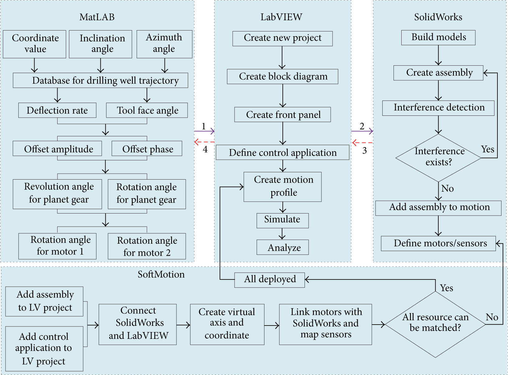
Simulation flowchart with SolidWorks, LabVIEW, and the SoftMotion module.

Before the simulation runs, input parameters were calculated in MATLAB. According to the known parameters, deflection rates and tool face angles of the steering mechanism could be deduced. Further, refering to the method presented in Section 2.2, revolution and rotation angles of the planet gear could be achieved. Finally, the rotation angles of the two motors could be calculated. When all calculations were completed, input parameters were stored in text file format preparing for later simulation.

The control application for the simulation was created in LabVIEW with SoftMotion. And the control application mainly consists of data read module, parameters set module, and results displayed module. The data read module reads input parameters for the simulation. The parameters set module is used to set control parameters for the simulation. The results displayed module displays the simulation results. Control application for the simulation is shown in Figure 7.

Figure 7:

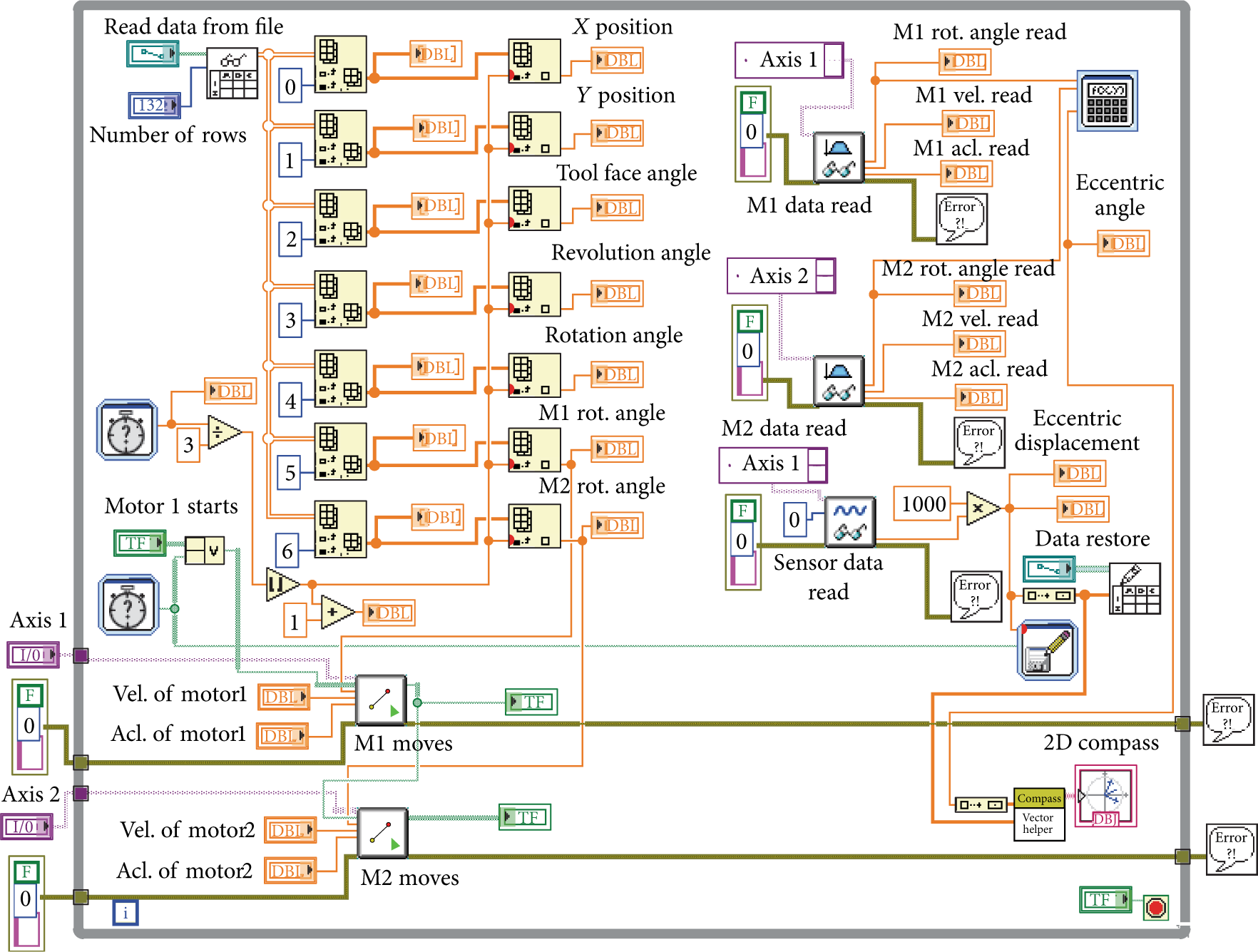
LabVIEW control application for motion control and simulation.

The 3D model of the steering mechanism for the simulation was built in SolidWorks. When interference detection is completed, the assembly model was imported into SolidWorks Motion module. In the Motion module, virtual axes for rotation drive were added and virtual sensors were defined. The simplified 3D model for simulation is shown in Figure 8.

Figure 8:

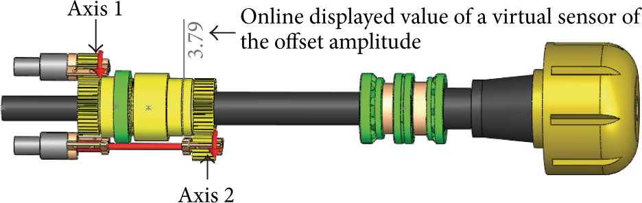
The simplified and set 3D model for simulation.

NI SoftMotion is mainly applied to control the motion of the 3D model in SolidWorks. With SoftMotion, the control application created in LabVIEW can be linked to SolidWorks, leading them to synchronize with each other. In SoftMotion, virtual axis and sensors should be defined and matched. When all motors and sensors are found and matched correctly, the motion profile can be created and the simulation will be ready.

When the simulation runs, input parameters are read by LabVIEW as presented by Step 1 shown in Figure 6. During the simulation process, the motion of 3D model in SolidWorks is controlled by LabVIEW as presented by Step 2. In the meanwhile, the simulation results obtained by virtual sensors in SolidWorks are sent to LabVIEW as presented by Step 3. After the simulation is completed, the actual well trajectory is drawn in MATLAB as presented by Step 4. By comparing the ideal well trajectory and the actual well trajectory, the steering performance analysis of the new steering mechanism can be achieved.

4.2. Motion Simulation for 2D Well Trajectory

2D well trajectory is located on a vertical plane, and the inclination angle changes continually while the azimuth angle keeps constant. A typical part of a 2D well trajectory is specified as

$y=\mathrm{1.25}{x}^{\mathrm{2}}+\mathrm{2.5}x\hspace{1em}\left(x\in \left[\mathrm{0,12}\right]\right).$

(17)

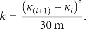
Target points on the curve are obtained by sampling every 30 m [27]. Further, the inclination angle (κ) of each target point can be calculated as

$\kappa =\arctan \left(y^{\prime }\right)=\arctan \left(\mathrm{2.5}x+\mathrm{2.5}\right)\hspace{1em}\kappa \in \left[\mathrm{0},\frac{\pi }{\mathrm{2}}\right].$

(18)

And then, the deflection rate (k) between two adjacent target points is

$k=\frac{{\left({\kappa }_{\left(i+\mathrm{1}\right)}-{\kappa }_i\right)}^{\circ }}{\mathrm{30}\hspace{0.17em}\text{m}}.$

(19)

Once the deflection rate is calculated, the deviation angle of the drilling mandrel can be deduced refering to “Modified Three Point Geometry Method.” According to “Modified Three Point Geometry Method,” the ideal well trajectory between two adjacent target points can be approached by a circular arc of actual drilling well trajectory. The circular arc passing through three support points of the new steering mechanism and its curvature is specified as the same as that of the ideal well trajectory [28]. The schematic of the “Modified Three Point Geometry Method” principle to calculate the deviation angle of the drilling mandrel is shown in Figure 9.

Figure 9:

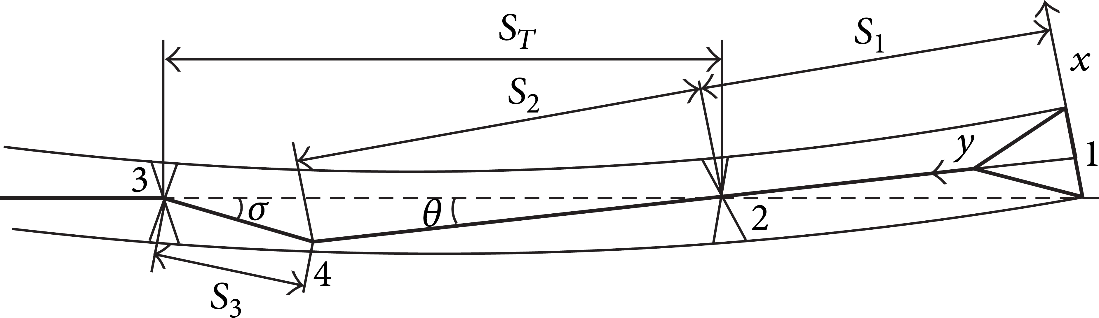
Schematic of the “Modified Three Point Geometry Method” principle.

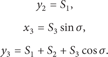
In Figure 9, points 1, 2, 3, and 4 are, respectively, the center of drill bit, bottom stabilizer, upper stabilizer, and bottom universal joint. Points 1, 2, and 3 are the support points of the new steering mechanism against the well wall and they determine the circular arc of the actual well trajectory. In the schematic above, S₁, S₂, and S _T are the known quantities; S₃ and σ are the variables; θ is the aim parameter. The process to calculate the deviation angle of the drilling mandrel is as follows.

Take point 1 as the origin to establish the coordinate system, and then the following equations can be obtained:

$\begin{array}{c}{y}_{\mathrm{2}}=S_{\mathrm{1}},\\ x_{\mathrm{3}}=S_{\mathrm{3}}\sin \sigma ,\\ y_{\mathrm{3}}=S_{\mathrm{1}}+S_{\mathrm{2}}+S_{\mathrm{3}}\cos \sigma .\end{array}$

(20)

Then the curvature of the circular arc (ξ) can be expressed as

$\begin{array}{l}\xi =\frac{\mathrm{2}\left|x_{\mathrm{3}}\right|}{\sqrt{{\left(x_{\mathrm{3}}{y}_{\mathrm{2}}\right)}^{\mathrm{2}}+{\left(x_3^2+y_2^2-y_{\mathrm{2}}{y}_{\mathrm{3}}\right)}^{\mathrm{2}}}}\\ =\mathrm{2}{S}_{\mathrm{3}}\sin \sigma \times (\phantom{{+S_{\mathrm{1}}\left(S_{\mathrm{2}}+S_{\mathrm{3}}\cos \sigma \right)\phantom{S_2^2}]}^2}{S}_1^2{S}_3^2\text{si}{\text{n}}^{\mathrm{2}}\sigma +[S_2^2+\mathrm{2}{S}_{\mathrm{2}}{S}_{\mathrm{3}}\cos \sigma +S_3^2{{+S_{\mathrm{1}}\left(S_{\mathrm{2}}+S_{\mathrm{3}}\cos \sigma \right)\phantom{S_2^2}]}^2)}^{-1/2}.\end{array}$

(21)

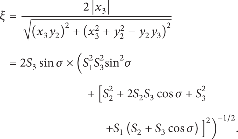
As σ is small enough, suppose that sinσ = σ, cos⁡σ = 1, and the expression above approximately equals the following:

$\xi =\frac{\mathrm{2}{S}_{\mathrm{3}}\sigma }{\left(S_{\mathrm{2}}+S_{\mathrm{3}}\right)\left(S_{\mathrm{1}}+S_{\mathrm{2}}+S_{\mathrm{3}}\right)}.$

(22)

Further, the deflection rate of the new steering mechanism can be calculated as follows:

$k=\mathrm{30}\hspace{0.17em}\xi =\frac{{\left(\mathrm{60}{S}_{\mathrm{3}}\sigma /\left(\left(S_{\mathrm{2}}+S_{\mathrm{3}}\right)\left(S_{\mathrm{1}}+S_{\mathrm{2}}+S_{\mathrm{3}}\right)\right)\right)}^{\circ }}{\mathrm{30}\hspace{0.17em}\text{m}}.$

(23)

Refering to the cosine and sine theorem, S₃ and σ can be expressed as follows:

$\begin{array}{c}{S}_{\mathrm{3}}=\sqrt{S_T^2+S_2^2-\mathrm{2}{S}_T{S}_{\mathrm{2}}\cos \theta },\\ \frac{\sin \sigma }{S_{\mathrm{2}}}=\frac{\sin \theta }{S_{\mathrm{3}}}⟹\sigma \approx \sin \sigma =\frac{S_{\mathrm{2}}\sin \theta }{S_{\mathrm{3}}}.\end{array}$

(24)

As θ is also small enough, suppose that cos θ = 1 and sin θ = θ. And, hence, the deflection rate can be further expressed:

$k=\frac{\mathrm{60}{S}_{\mathrm{2}}\theta }{S_T\left(S_{\mathrm{1}}+S_T\right)}.$

(25)

In this new steering mechanism, the parameters of S₁, S₂, and S _T are, respectively, assigned as S₁ = 600 mm, S₂ = 1000 mm, and S _T = 1200 mm. As a result, the deflection rate can be finally expressed:

$k=\frac{{\left(\mathrm{10.7}\theta \right)}^{°}}{\mathrm{30}\hspace{0.17em}\text{m}}.$

(26)

Once the deflection rate (k) is calculated, the deviation angle (θ) can be deduced. Further, the offset amplitude of the offset point can be calculated as

$d=\theta S_{\mathrm{2}}.$

(27)

As the azimuth angle keeps constant during the drilling process, the offset phase of the offset point always keeps constant at 270°. And hence the eccentric displacement vector for each point can be calculated.

According to the kinematic solution presented in Section 2.2 and the procedures and program architectures for the motion simulation presented in Section 4.1, the input parameters for simulation can be calculated. In the 2D well trajectory motion simulation, suppose that there are six target points. The input parameters for the motion simulation are shown in Table 2.

Table 2:

Parameters for 2D well trajectory motion simulation.

	A	B	C	D	E	F
X (m)	3.97	5.98	7.52	8.83	9.98	11.03
Y (m)	29.68	59.62	89.58	119.55	149.52	179.51
L (m)	30	60	90	120	150	180
κ (°)	4.55	3.24	2.64	2.29	2.04	1.86
d (mm)	0.430	1.331	0.601	0.361	0.247	0.183
α (°)	87.65	−4.94	4.00	1.31	0.62	0.35
δ (°)	−101.11	−4.44	3.60	1.18	0.56	0.32
λ1 (°)	205.47	9.03	−7.32	−2.40	−1.13	−0.64
λ2 (°)	−195.93	11.03	−8.95	−2.93	−1.39	−0.78

In Table 2, the minus represents that the rotation direction is opposite to the initially defined. Import these parameters into LabVIEW, set control parameters, and run the simulation. When the simulation starts, the 3D model in SolidWorks will move under the control of LabVIEW. From front panel, the curve of offset amplitude of the offset point on the drilling mandrel can be achieved. Then, the actual drilling well trajectory can be drawn based on the principle of “Modified Three Point Geometry Method.” The curve of the offset amplitude is shown in Figure 10. The actual drilling well trajectory, the ideal well trajectory, and the curve of 10* error (error multiplied by 10 to be shown clearly) are shown in Figure 11.

Figure 10:

Eccentric displacement for 2D well trajectory simulation.

Figure 11:

The actual and the ideal well trajectories of 2D well trajectory motion simulation.

Figure 10 shows the adjustment process of the eccentric displacement of the offset point on the drilling mandrel during drilling the 2D well trajectory. The eccentric displacement is adjusted by the new steering mechanism at each target point and then it will keep the constant until reaching next adjacent target point. In Figure 10, the simulation curve of the offset amplitude shows that the results acquired by simulation are the same as those acquired by mathematical calculation listed in Table 2. As presented in Figure 11, the actual well trajectory passes through each target point and it approaches the ideal well trajectory nearly, especially the parts after point A. The error curve shows that the error between the actual well trajectory and the ideal well trajectory from point A to point B are more obvious and larger than those of other parts. The maximum of the error appears at the position of x = 2, where the value of error is d_max = 47.5/10 = 4.75 m. The explanation for the error from point A to point B is that the rotation angles of the two motors from the initial state are much larger than those of other parts. And the adjustment process for this part takes more time. For RSS drilling a 2D well trajectory, the error in this simulation is within the accepted range (d ≤ 10 m) [29]. And hence the new steering mechanism can satisfy the directional steering need for 2D well trajectory.

4.3. Motion Simulation for 3D Well Trajectory

3D well trajectory is a curve in space, which means that the inclination angle and azimuth angle are both changing continuously. For 3D well trajectory, the coordinate values, inclination angles, well depths, and azimuth angles of the target points are already known. Based on these known parameters, input parameters for the 3D well trajectory simulation can be calculated refering to the principle of “Limiting Curvature Method.” According to the principle of “Limiting Curvature Method,” the well trajectory between two adjacent target points is a circular arc and the circular arc is on an incline plane [30]. The process for the input parameters calculation is shown as follows.

Firstly, the deflection rate (k_{i(i + 1)}) of the new steering mechanism between two adjacent target points i and i + 1 can be calculated:

$\begin{array}{c}{\gamma }_{i\left(i+\mathrm{1}\right)}\hspace{1em}=\text{arccos}[\phantom{\left({\phi }_{\left(i+\mathrm{1}\right)}-{\phi }_i\right)}\cos {\kappa }_i\cos {\kappa }_{(i+\mathrm{1})}+\sin {\kappa }_i\sin {\kappa }_{\left(i+\mathrm{1}\right)}\cos \left({\phi }_{\left(i+\mathrm{1}\right)}-{\phi }_i\right)],\\ k_{i\left(i+\mathrm{1}\right)}=\frac{\mathrm{30}{\gamma }_{i\left(i+\mathrm{1}\right)}}{\left(L_{\left(i+\mathrm{1}\right)}-L_i\right)},\end{array}$

(28)

where γ_{i(i + 1)} is the whole angle of the circular arc between the target points i and i + 1; κ _i and κ_{(i + 1)} are the inclination angles; φ _i and φ_{(i + 1)} are the azimuth angles; L _i and L_{(i + 1)} are the well depth.

Further, the tool face angle (ω _i ) of the new steering mechanism at each target point can be obtained:

$\begin{array}{c}{R}_{i\left(i+\mathrm{1}\right)}=\frac{\left(L_{\left(i+\mathrm{1}\right)}-L_i\right)}{{\gamma }_{i\left(i+\mathrm{1}\right)}},\\ \cos {\omega }_i=\frac{\cos {\kappa }_i\sin {\kappa }_{\left(i+\mathrm{1}\right)}\cos \left({\phi }_{\left(i+\mathrm{1}\right)}-{\phi }_i\right)-\sin {\kappa }_i\cos {\kappa }_{\left(i+\mathrm{1}\right)}}{\sin {\gamma }_{i\left(i+\mathrm{1}\right)}},\\ \sin {\omega }_i=\frac{\sin {\kappa }_i\sin \left({\phi }_{\left(i+\mathrm{1}\right)}-{\phi }_i\right)}{\sin {\gamma }_{i\left(i+\mathrm{1}\right)}},\\ {\omega }_i=\{\begin{array}{cc}\text{arccos}\left(\cos {\omega }_i\right),\hfill & \left(\sin {\omega }_i\ge \mathrm{0}\right),\hfill \\ \mathrm{2}\pi -\text{arccos}\left(\cos {\omega }_i\right),\hfill & \left(\sin {\omega }_i<\mathrm{0}\right),\hfill \end{array}\end{array}$

(29)

where R_{i(i + 1)} is the radius of the circular arc.

Further, input parameters for the 3D well trajectory simulation will be obtained according to the kinematic solution presented in Section 2.2 and the procedures and program architectures for the motion simulation presented in Section 4.1. The known parameters (X,Y,Z,L,κ,φ) and the input parameters (d,ω,α,β,λ₁,λ₂) are listed in Table 3.

Table 3:

Parameters for 3D well trajectory motion simulation.

	A	B	C	D	E	F
X (m)	0	10	50	200	250	250
Y (m)	0	0	10	60	90	90
Z (m)	1000	1150	1350	1600	1800	2300
L (m)	1000	1200	1500	1800	2000	2300
κ (°)	0	15	30	20	0	0
φ (°)	0	0	20	20	20	20
d (mm)	2.273	1.682	1.516	3.032	0	Null
ψ (°)	270	226.06	270	270	270	Null
α (°)	−77.491	194.923	−199.132	8.486	73.214	Null
δ (°)	110.258	102.131	−105.918	7.637	−114.108	Null
λ1 (°)	−224.054	−207.534	215.234	−15.518	231.877	Null
λ2 (°)	173.215	−435.710	445.118	−18.868	−163.655	Null

According to the principle of “Limiting Curvature Method,” another medium target point (j) between the target points i and i + 1 is needed to define the circular arc of the actual well trajectory on the incline plane. The coordinate values of j can be calculated as

$\begin{array}{c}\iota =\frac{L_j-L_i}{R_{i\left(i+\mathrm{1}\right)}},\\ X_j=X_i+R_{i\left(i+\mathrm{1}\right)}\times [\sin {\kappa }_i\cos {\phi }_i\sin \iota +\left(\cos {\kappa }_i\cos {\phi }_i\cos {\omega }_i-\sin {\phi }_i\sin {\omega }_i\right)\times \left(\mathrm{1}-\cos \iota \right)],\\ Y_j=Y_i+R_{i\left(i+\mathrm{1}\right)}\hspace{1em}\times [\sin {\kappa }_i\sin {\phi }_i\sin \iota +\left(\cos {\kappa }_i\sin {\phi }_i\cos {\omega }_i+\cos {\phi }_i\sin {\omega }_i\right)\times \left(\mathrm{1}-\cos \iota \right)],\\ Z_j=Z_i+R_{i\left(i+\mathrm{1}\right)}\times \left[\cos {\kappa }_i\sin \iota -\sin {\kappa }_i\cos {\omega }_i\left(\mathrm{1}-\cos \iota \right)\right],\end{array}$

(30)

where ι is a medium variable.

In 3D well trajectory simulation, the number of the target points is specified as six.

Import these parameters into LabVIEW, and run the simulation. From front panel, the offset amplitude and phase of the offset point can be obtained. According to data acquired by simulation, actual drilling well trajectory can be deduced based on the principle of “Limiting Curvature Method.” The offset amplitude and offset phase are shown in Figure 12. The actual drilling well trajectory is shown in Figure 13.

Figure 12:

The offset amplitude and offset phase of the drilling mandrel in the simulation.

Figure 13:

The actual drilling trajectory of the 3D well trajectory motion simulation.

Figure 12 shows the adjustment process of the eccentric displacement vector (expressed by the offset amplitude and the offset phase) of the offset point on the drilling mandrel during drilling the 3D well trajectory. The eccentric displacement vector is adjusted by the new steering mechanism at each target point and then it will keep the constant until reaching the next adjacent target point. In Figure 12, the simulation curves show that the offset amplitudes and the offset phases acquired by the simulation between two adjacent target points are the same as those acquired by mathematical calculation listed in Table 3. As presented in Figure 12, the adjustment processes of the offset amplitude and the offset phase are performed simultaneously to ensure that they can reach the needed values at the same time. And hence the adjustment process is more complicated and takes more time as shown in Figure 12.

As presented in Figure 13, the actual well trajectory passes through the six specified target points in the space. And the actual drilling well trajectory consists of six portions. The first portion (before point A) is a vertical line and the steering mechanism will not offset the drilling mandrel. The second portion (from point A to point B) is a circular arc on the vertical plane, meaning that the inclination angles are increasing while the azimuth angles keep constant. When drilling this portion, the state of the steering mechanism is similar to drilling a 2D well trajectory. The third portion (from point B to point C) is a circular arc on an incline plane, meaning the inclination angles and azimuth angles both increasing continually. The fourth portion (from point C to point D) and fifth portion (from point D to point E) are similar in that the inclination angles are decreasing and the azimuth angles keep constant. Both the two portions are circular arcs on a vertical plane. The last portion (from point E to point F) is a vertical line that is the same as the first portion. The 3D well trajectory motion simulation shows that the new steering mechanism can satisfy the drilling need for drilling complicated 3D well trajectories.

5. Prototype Experiments

To verify the steering performance of the new mechanism, a prototype was built as shown in Figure 14.

Figure 14:

The steering control experiment for the prototype of the new steering mechanism.

Steering control experiments were then conducted using the prototype. In the experiments, the eccentric displacement vector of the offset point on the drilling mandrel is expressed by the X and Y coordinates of the offset point. The control system is constructed according to Figure 5. An NI PCI-7354 card acts as the motion control module. Two displacement sensors are used to monitor separately the offset displacements of the drilling mandrel along x- and y-axes. An NI USB-6356 DAQ module is used to acquire the data of the two displacement sensors and transfer the data to the industrial control computer.

In the steering control experiment, the rotation angles of the two DC servomotors are the input parameters, and 13 pairs of input data are chosen as shown in Table 4.

Table 4:

Input parameters for the steering control experiment.

	t = 0 s	60 s	120 s	180 s	240 s	300 s	360 s	420 s	480 s	540 s	600 s	660 s	720 s
λ1 (°)	0	0	15	0	30	0	45	0	90	0	180	0	360
λ2 (°)	0	15	0	30	0	45	0	90	0	180	0	360	0

The X and Y coordinates of the offset point on the drilling mandrel for the prototype experiment and the computer simulation are, respectively, shown in Figures 15 and 16.

Figure 15:

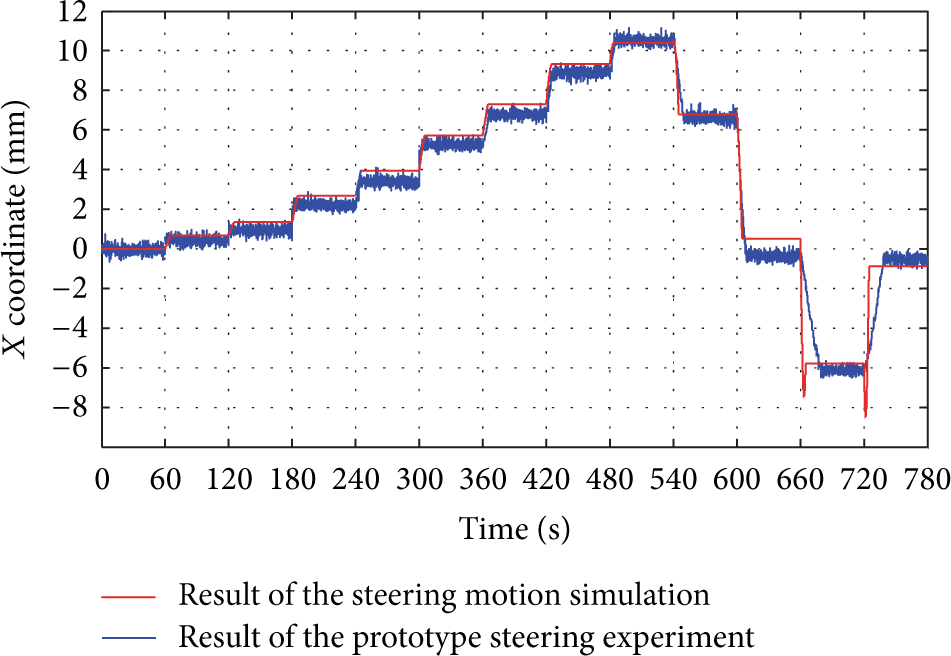
The X coordinates of the offset point for the prototype experiment and simulation.

Figure 16:

The Y coordinates of the offset point for the prototype experiment and simulation.

As presented in Figures 15 and 16, the experiment results match the simulation results well. However, there are notable deviations for several positions, for example, at the time of 630 s. Such deviations may be attributed to a number of factors, for example, sensor accuracy, part dimension tolerances, and gravity force. Further calibration experiments may help improve the accuracy. Note that the fluctuation of the X and Y coordinates in the prototype experiment is due to the vibration of the rotating drilling mandrel. The experiments verify the correctness of the steering principle analysis, theoretical calculation, and steering motion simulation.

6. Conclusion

In this study, a new steering mechanism based on a set of hollow universal joints and a set of specific planetary gear small tooth number differences (PGSTD) for the point-the-bit rotary steerable system (RSS) is proposed. The new steering mechanism has a compact structure and is easy to operate. It modifies several previous ideas of achieving directional steering and may better meet the demands in rotary steerable drilling. The principle of the new steering mechanism was presented. The structural design and control system design of the mechanism were described in detail. To analyze its steering performances, the eccentric displacement vector of the drilling mandrel was analyzed and formulated. Motion simulations for 2D and 3D well trajectories were conducted to verify the working principle and the accuracy of the kinematic solutions using LabVIEW and SolidWorks. The simulations showed that the new steering mechanism could achieve directional drilling and satisfy the drilling needs for complicated well trajectories. Steering control experiments for a prototype of the new steering mechanism verify the correctness of the theoretical calculation and steering motion simulation. However, due to the limitations of time and conditions, the prototype experiments are still limited to run in the laboratory. Real drilling experiments under actual drilling conditions will be beneficial to evaluate the effectiveness of the new mechanism. Moreover, the dynamic performance of the new steering mechanism should be optimized to meet the challenge of complicated underground environments. This work of paper is expected to provide useful guidance for the design and research of the steering mechanism for the point-the-bit RSS.