Sage Journals: Discover world-class research

Abstract

U-type tubes are widely used in military and civilian fields and the quality of the internal surface of their channel often determines the merits and performance of a machine in which they are incorporated. Abrasive flow polishing is an effective method for improving the channel surface quality of a U-type tube. Using the results of a numerical analysis of the thermodynamic energy balance equation of a two-phase solid-liquid flow, we carried out numerical simulations of the heat transfer and surface processing characteristics of a two-phase solid-liquid abrasive flow polishing of a U-type tube. The distribution cloud of the changes in the inlet turbulent kinetic energy, turbulence intensity, turbulent viscosity, and dynamic pressure near the wall of the tube were obtained. The relationships between the temperature and the turbulent kinetic energy, between the turbulent kinetic energy and the velocity, and between the temperature and the processing velocity were also determined to develop a theoretical basis for controlling the quality of abrasive flow polishing.

1. Introduction

Abrasive flow machining is a polishing method by which the pressure applied by the back-and-forth flow of a soft abrasive viscoelastic medium is used to polish the surface of the machined part [1]. The hard and sharp edges of the grains in the abrasive flow are used as cutting tools for achieving a certain degree of polishing. The advantage of abrasive flow machining is its applicability to channels that cannot be easily accessed by general tools [2, 3]. The even and progressive abrasion of the surface and corners of the worked parts by the grains can be used to accomplish deburring, polishing, and chamfering. It has been experimentally confirmed that abrasive flow machining can be used to significantly improve the surface quality of nonlinear runners [4]. The machining mechanism is illustrated in Figure 1.

Figure 1:

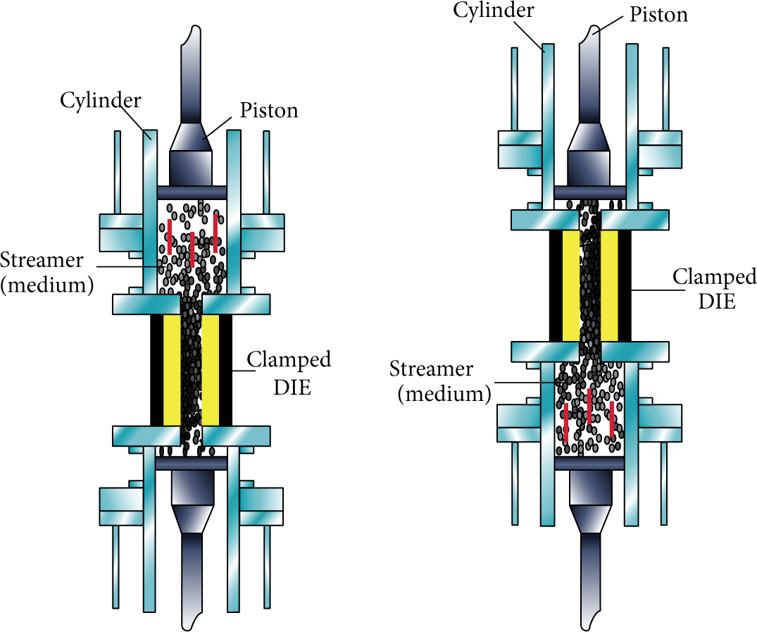
Principle of abrasive flow machining.

Several studies on abrasive flow machining have been conducted and reported. Jain et al. [5 –9] experimentally investigated the effect of the central force on the process and obtained the relationship among the shaft velocity, cycle index, and grain size, with the purpose of improving the surface roughness of the grain and the material removal. They also investigated the modeling of the abrasive media by modifying the standard Maxwell model of elastomers to the generalized Maxwell model. With the assumption that the material removal by shear stressing was dependent on the bonding of the abrasive grains, a fundamental material model that could be easily integrated in conventional simulation programs was developed and presented. Sankar et al. [10 –12] also discussed the effect of rotating abrasive flow machining on the surface morphology of the workpiece and analyzed the relationship between the rotational velocity of the workpiece and the effective abrasion distance in the polishing area using the theoretical and experimental spiral path lengths. They also obtained the relationship among the rotational velocity of the workpiece, the rate of change of the surface roughness, and the amount of removed material. Furumoto et al. [13] studied the interior of the injection mold used for free abrasive finishing machining and found that high-velocity free-flowing abrasion increases the kinetic energy of the grains, which in turn increases the possibilities of contact between the grains and the inner surface, thereby improving the polishing quality. Kar et al. [14] put forward a method for measuring the axial force of single abrasive flow polishing of AISI4140, a material used for automobile hydraulic cylinders. They investigated the effect of the medium pressure and processing time on the surface quality of the workpiece. Ji et al. [15, 16] used the Preston equation and its modified coefficient of VOF to model the softness of the structural surface of an abrasive flow. By numerical simulation, they found that the average velocity of the abrasive particles in the tube line increased with increasing inlet flow rate. Using the cutting experience formula for soft abrasive flow, the Euler multiphase flow model, and the realizable k-ε turbulence model of a V-type textural semiannular liquid-solid flow with different particle concentrations, they performed numerical simulations to investigate the turbulent velocity for different types of particles. By examining the wall pressure, they determined the optimum particle size for soft abrasive flow polishing and also found that the shape and structure of the microchannel significantly affected the process. Wan et al. [17] proposed a simple zero-order semimechanistic approach to the analysis of two-way abrasive flow machining. This was prompted by the need to reduce the number of time-consuming and labor-intensive experimental trials.

Wang et al. [18] also used a numerical method to design effective passageways for producing a smooth surface in a complex hole by abrasive flow machining. They examined the current method and found that the shear forces of the polishing process and the flow properties of the machining medium determined the smoothness of the entire surface.

In the present study, the existing theory was examined and simulation experiments were performed under specific conditions. The study was prompted by the fact that unless the grinding viscosity temperature characteristics of the particle flow of abrasive flow polishing are determined and the relevant quality relationships are established, the existing theory would remain incomplete and there would be limited universal guidelines for the process. In this study, the effects of the viscosity temperature characteristics of abrasive flow polishing on the quality of the produced surface were investigated with the purpose of developing the relationships among the process temperature, turbulent kinetic energy, turbulence intensity, velocity, and dynamic pressure. It is expected that such would be used to improve the polishing quality of the process and further develop its theory.

2. Numerical Thermodynamic Model of Two-Phase Solid-Liquid Flow

In the mass conservation and momentum conservation equations, the pressure and velocity are unknown physical parameters. In a two-phase solid-liquid flow, the viscosity and density often change, and the dynamic viscosity of the fluid medium can be determined when large temperature changes occur. The density of a liquid is significantly related to its compressibility, and variations in the density can be ignored for small compressibilities. Hence, the energy conservation equation can be used to determine the temperature at each point in a flow field based on the other variables, which include the pressure and velocity.

2.1. Energy Conservation Equation

The energy conservation law is a basic law that a flow through a heat exchange system is required to satisfy. The law states that the energy of an element in a fluid flow is equal to the net increase in energy of the element plus the physical work done on it by the surface forces:

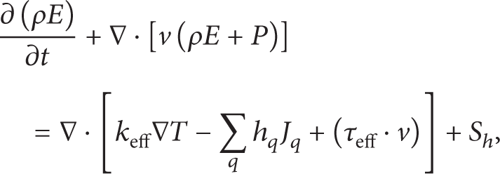
\begin{array}{l} \frac{\partial (ρ E)}{\partial t} + \nabla \cdot [v (ρ E + P)] \\ = \nabla \cdot [k_{eff} \nabla T - \sum_{q} h_{q} J_{q} + (τ_{eff} \cdot v)] + S_{h}, \end{array}

(1)

where E represents the kinetic energy and internal energy of the fluid element: E = h − (P/ρ) + (v²/2). In an abrasive flow, the compressibility is small; hence, the enthalpy is given by h = ∑_qY_qh_q + (P/ρ), where Y_q is the mass fraction of the q phase. The specific enthalpy of the q phase can be expressed as $h_{q} = \int_{T_{ref}}^{T} c_{p, q} d T$ , where C_p,q is the specific heat capacity of the q phase, T_ref = 298.15 K, k_eff is the effective thermal conductivity of the fluid, and J_q is the diffusion flux of the q phase. The first three terms on the right-hand side of (1) are, respectively, the thermal, diffusion, and viscous dissipation terms of the energy transfer, and S_h may be the internal heat of the source fluid, the exothermic or endothermic heat of a chemical reaction, or some other custom term.

2.2. Particle Temperature Equation

The development of science and technology over recent years has led to the use of the dynamic theory to determine the viscosity coefficient, thermal conduction coefficient, particle phase pressure, and other parameters. This has resulted in the development of the particle temperature equation. In abrasive flow machining, the collision between the abrasive particles and the wall surface due to the irregular motion of the particles is similar to the thermal motion of fluid molecules. The abrasive particles in a turbulent two-phase flow continuously gain energy, but their inelastic collisions with the wall also results in constant dissipation of energy. The particle temperature equation can therefore be suitably applied to the energy variation of the particles of a two-phase liquid-solid flow:

\begin{array}{l} \frac{3}{2} [\frac{\partial}{\partial t} (α_{s} ρ_{s} T_{s}) + \nabla \cdot (α_{s} ρ_{s} v_{s} T_{s})] \\ = (- P_{s} [I] + τ_{s}) : \nabla v_{s} - γ_{s} + \nabla \cdot (k_{s} \nabla T_{s}) - 3 C_{D} α_{s} T_{s}, \end{array}

(2)

where the left-hand side of the equation represents the accumulated kinetic energy of the particles and the right-hand side is obtained from the granular temperature convection transport equation. The first term on the right-hand side is the granular stress deformation work, the second term is the energy dissipation of the particles due to their inelastic collision with the wall, the third term is the thermal conductivity of the particles, and the last term represents the effect of the energy dissipation of the fluid and solid phases.

In (2), P_s and τ_s are, respectively, the compressive and shear stresses of the particulate phase, K_s is the heat conduction coefficient of the particles, and γ_s is the particle collision energy dissipation term:

\begin{array}{l} k_{s} = \frac{150 ρ_{s} d_{s} \sqrt{π T_{s}}}{384 (1 + e) g_{0}} {[1 + \frac{6}{5} α_{s} g_{0} (1 + e)]}^{2} + 2 ρ_{s} α_{s}^{2} d_{s} (1 + e) g_{0} \sqrt{\frac{T {}_{s}}{π}} \\ γ_{s} = \frac{12 (1 - e^{2})}{d_{s} \sqrt{π}} ρ_{s} α_{s}^{2} g_{0} \sqrt{T_{s}^{3}} . \end{array}

(3)

It can be seen from the granular temperature equation that the solid particles maintain laminar flow while the turbulent liquid phase gains energy and then dissipates it through inelastic collision with the wall surface. The turbulent particle phase is separated from the single-particle fluctuation zone by the single particle fluctuation characteristics produced by the inelastic collision of the randomly moving particles with the wall. The turbulent fluctuation of the particle phase reflects the turbulent fluctuation behavior of the solid particles. The particle temperature is determined by the single particle level, and the turbulent kinetic energy of the particles and the granular temperature may therefore be reduced by the dissipation of turbulent kinetic energy. The ultimate dissipative state particle temperature is irreversibly transformed into heat, which determines the particle temperature in a thermodynamic sense.

3. Development of Physical Model of U-Type Tube

3.1. Energy Conservation Equation

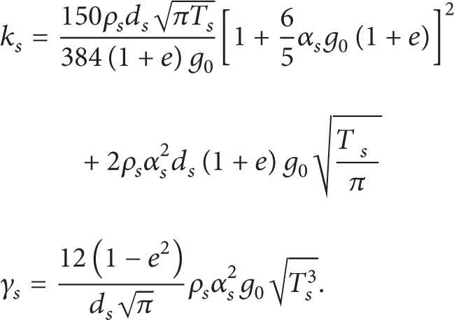
In this study, a U-type tube was used as the object of the numerical thermodynamic analysis of abrasive flow polishing. The tube is shown in Figure 2(a). Based on the characteristics of a two-phase solid-liquid abrasive flow polishing channel determined by simulation, the actual channel geometry model of a U-type tube requires simplification. The simplified geometry model is shown in Figure 2(b).

Figure 2:

U-type tube model.

3.2. Energy Conservation Equation

Because the abrasive flow polishing medium in a U-type tube contains a viscous fluid, investigation of the heat transfer during the process requires an analysis of the flow field parameters, including the dynamic pressure and the turbulent kinetic energy of the machined parts near the wall. The structure of the inner channel of a U-type tube is relatively simple; using an unstructured hexahedral mesh, the mesh division is as shown in Figure 3.

Figure 3:

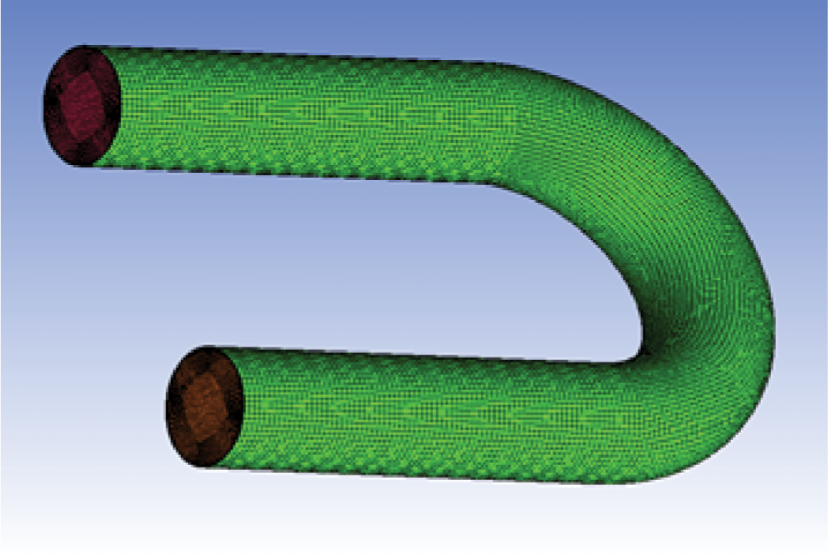
Mesh of U-type tube.

The flow of abrasive flow machining is complex and involves strong fluctuations between laminar and turbulent flows. The numerical simulation of the turbulent flow is more vulnerable to the grid than that of the laminar flow. To ensure accurate turbulence calculations, the area of the boundary layer where the average flow changes quickly and the average stress is large is selected as the near-wall region. To deal with the calculation mesh, a boundary layer is added to the part of the flow region near the wall, and the flow region is divided into specific regions between the surface mesh and the internal mesh. The grid independence check has been done. After grid independence check, U-type model is divided into 541896 nodes, with 530796 hexahedral cells, 1581589 quadrilateral interior faces, and 17622 quadrilateral wall faces. The grid volume is positive.

Based on the characteristics of abrasive flow machining, ICEM, which is the preprocessing module of FLUENT, was used in this study to develop the geometry of the flow region, set the boundary type, and generate the meshes on the parts of the U-type tube. A noncoupled implicit double precision solver was used for the numerical analysis of the turbulent RNG k-ε model of the two-phase solid-liquid turbulent flow. An abrasive flow media carrier was used as the main phase and silicon carbide particles with a volume score of 0.3 mm were used as the secondary phase. The boundary conditions and the inlet and outlet velocities were set, and the rest of the wall was considered to be solid. The effects of gravity were taken into consideration.

After setting the parameters, the SIMPLEC algorithm was used to solve the dynamic two-phase flow equation and perform the calculations in the flow area. After initialization, iterative computations were used to analyze the abrasive flow machining process in the U-type tube. Using the calculation results, we obtained the residual monitoring curve and some numerical simulation figures.

4. Results and Discussion

The simulated U-type tube had an internal diameter of 4 mm and the first introduction of turbulent kinetic energy was under a condition different from that of a U-type tube used for abrasive flow machining. For an inlet velocity of 70 m/s and initial temperature of 300 K, we analyzed the turbulent kinetic energy in the near-wall region, as well as the turbulence intensity, turbulent viscosity, and dynamic pressure nephrogram. Figure 4 shows the images of the turbulent kinetic energy in the U-type tube for different inlet conditions. Figure 5 shows the turbulence intensity at the corners and near the tube exit, and it can be observed that the values are relatively large near the wall and reach a maximum at the corner. The U-type tube channel abrasive flow has a polishing effect at the bend in the tube where the irregular motion of the abrasive grains is more intense. Figures 4 –7 show the turbulent kinetic energy. (a), (b), and (c), respectively, correspond to 3.375, 9.375, and 13.5 m²/s².

Figure 4:

Turbulent kinetic energy cloud for different inlet conditions of U-type tube channel.

Figure 5:

Turbulence intensity images for different inlet conditions of U-type tube channel.

Figure 6:

Turbulent viscosity cloud for different inlet conditions of U-type tube channel.

Figure 7:

Dynamic pressure nephrogram under different entrance of turbulent kinetic energy of U-type tube channel.

It can be observed from Figure 6 that the turbulent viscosity near the wall of the channel was less than that at the centre and that near the wall in the bend was larger than that at the inner wall. The region of variable turbulent viscosity is relatively large because the abrasive flow into the channel has a microgrinding effect on the wall surface, and this increases the mean temperature near the wall. The decrease in the abrasive flow viscosity near the wall is greater than that at the center owing to the effects of eddy diffusion.

As can be seen from Figure 7, the dynamic pressure of the U-tube channel near the wall was very small, whereas those at the inlet and outlet at the corners were relatively large. For different inlet turbulent kinetic energy conditions near the wall, the distributions of the turbulence intensity, turbulent viscosity, and dynamic pressure can be divided into three sections, namely, the straight section after the inlet (section 1), the curved section (section 2), and the straight section before the outlet (section 3). In-depth comparative analyses of the distributions for different inlet turbulent kinetic energies near wall, turbulence intensities, turbulent viscosities, and dynamic pressures were conducted using a velocity of 70 m/s and initial temperature of 300 K. The distribution of the turbulent kinetic energy and turbulence intensities in the U-type tube are given in Table 1.

Table 1:

Distributions of turbulent kinetic energy and turbulence intensity in U-type tube for velocity of 70 m/s and initial temperature of 300 K.

Inlet turbulent kinetic energy (m²/s²)	Turbulent kinetic energy (m²/s²)			Turbulence intensity
Inlet turbulent kinetic energy (m²/s²)	section 1	section 2	section 3	section 1	section 2	section 3

3.375	150	285	235	1 000	1 240	1 102
9.375	160	290	245	1 140	1 370	1 240
13.5	171	308	257	1 200	1 442	1 302

An analysis of the data in Table 1 reveals that the turbulent kinetic energies and turbulence intensities in the different sections of the U-type tube increase with increasing inlet turbulent kinetic energy. It can also be observed from the table that, moving from section 1, through section 2, and to section 3, the turbulent kinetic energy and turbulence intensity increase and then decrease again. Comparative analyses reveal that, for an inlet turbulent kinetic energy of 9.375 m²/s², there was better uniformity in the turbulent kinetic energy and turbulence intensity in the tube channel. Table 2 gives the distributions of the turbulent viscosity and dynamic pressure in the tube for a velocity of 70 m/s and initial temperature of 300 K.

Table 2:

Distributions of turbulent viscosity and dynamic pressure in U-type tube for velocity of 70 m/s and initial temperature of 300 K.

Inlet turbulent kinetic energy (m²/s²)	Turbulent viscosity (kg/m·s)			Dynamic pressure (Mpa)
Inlet turbulent kinetic energy (m²/s²)	section 1	section 2	section 3	section 1	section 2	section 3

3.375	1.2	2.15	2.8	5.3	5.7	6.86
9.375	1.32	2.22	2.82	5.02	5.35	6.48
13.5	1.18	2.16	2.81	4.9	5.28	6.43

It can be observed from Table 2 that the turbulent viscosity initially increased with increasing inlet turbulent kinetic energy and then decreased. Moving from section 1, through section 2, and to section 3, the turbulent viscosity initially decreased and then increased. An examination of the dynamic pressure data in the table reveals that the dynamic pressure in the tube gradually decreased with increasing inlet turbulent kinetic energy, and that the dynamic pressure initially increased and then decreased with movement along the tube. Comparative analyses revealed that there was greater uniformity in the turbulent viscosity and dynamic pressure distributions for an inlet turbulent kinetic energy of 9.375 m²/s².

Using an inlet turbulent kinetic energy of 9.375 m²/s² and initial velocity of 70 m/s, U-type channel simulations were performed to evaluate the process for different distributions of the near-wall turbulence kinetic energy, turbulence intensity, turbulent viscosity, and dynamic pressure. In Figures 8 –11, (a), (b), (c), and (d), respectively, correspond to temperatures of 290, 300, 310, and 320 K.

Figure 8:

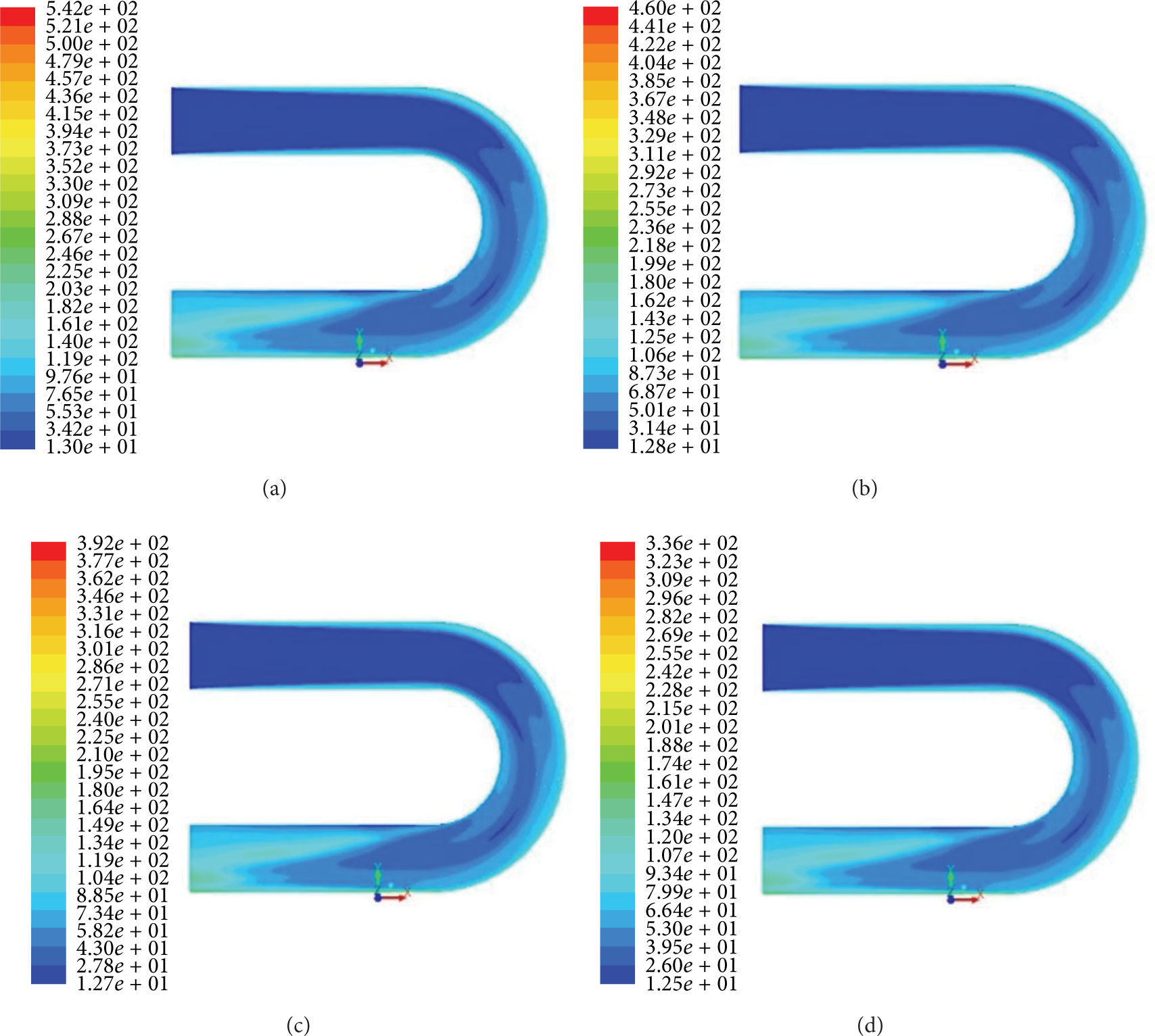
Turbulent kinetic energy cloud of U-type tube channel for different temperatures.

Figure 9:

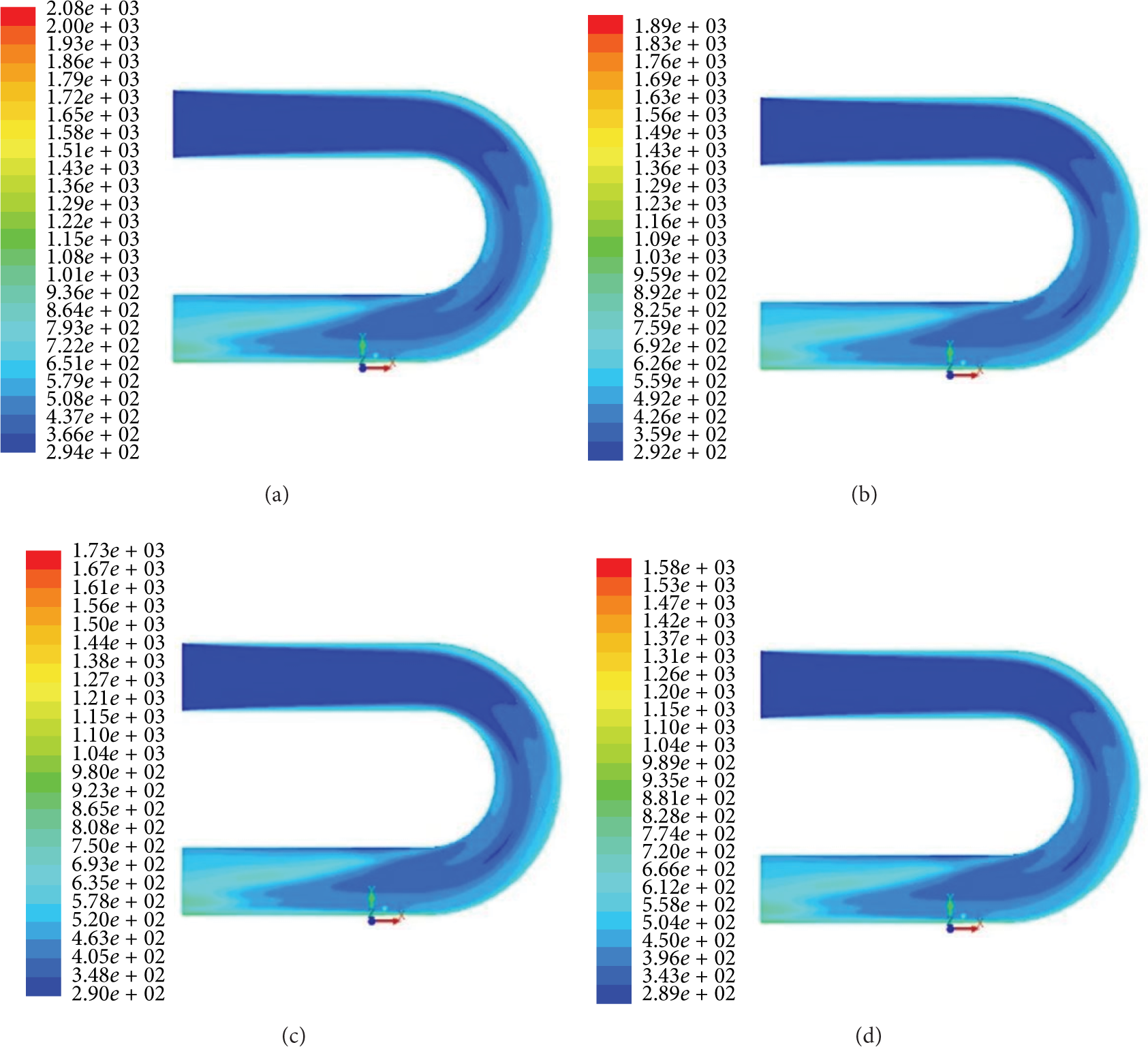
Turbulence intensity images of U-type tube channel for different temperatures.

Figure 10:

Turbulent viscosity cloud of U-type tube channel for different temperatures.

Figure 11:

Dynamic pressure nephrogram of U-type tube channel for different temperatures.

It can be seen from Figures 8 and 9 that the outlet turbulent kinetic energy and turbulence intensity near the wall around the bend of the tube were relatively high and attained maximum values at the bend. This indicates that the abrasive flow polishing mainly occurred around the bend of the U-type tube channel, which is conducive for light processing.

It can be observed from the images shown in Figure 10 that the change in the turbulent viscosity at the outer wall near the bend of the tube was greater than that at the outlet.

Figure 11 also reveals that the dynamic pressure of the U-type tube near the wall was very small, whereas those at the inlet and outlet were relatively large. The change in temperature had little effect on the dynamic pressure distribution. Based on the distributions of the near-wall turbulent kinetic energy, turbulence intensity, turbulent viscosity, and dynamic pressure for different temperatures, the U-type tube channel can be divided into three sections, namely, the straight section after the inlet (section 1), the curved section (section 2), and the straight section before the outlet (section 3). The distributions of the near-wall turbulent kinetic energy and turbulence intensity obtained by further comparative analyses for different temperatures using an inlet velocity of 70 m/s and turbulent kinetic energy of 9.375 m²/s² are given in Table 3.

Table 3:

Distribution of turbulent kinetic energy and turbulence intensity in U-type tube channel for inlet velocity of 70 m/s and turbulent kinetic energy of 9.375 m²/s².

Temperature(K)	Turbulent kinetic energy (m²/s²)			Turbulence intensity
Temperature(K)	section 1	section 2	section 3	section 1	section 2	section 3

290	192	330	280	1 190	1 430	1 290
300	160	290	245	1 140	1 370	1 240
310	145	280	230	1 110	1 345	1 210
320	134	272	220	1 090	1 330	1 190

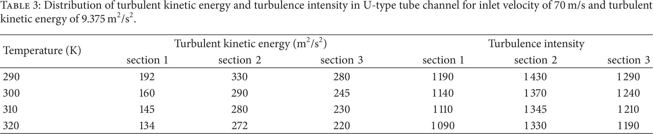
As can be seen from Table 3, the turbulent kinetic energy and turbulence intensity decreased drastically with increasing temperature. This was because the decrease in the viscosity of the abrasive flow medium with increasing temperature caused the velocity gradient of the liquid phase to decrease, thereby decreasing the turbulence intensity and turbulent kinetic energy. The turbulent kinetic energy and turbulence intensity initially increased between sections 1 and 2 and then decreased between sections 2 and 3. The distributions are, however, not uniform for any temperature. Table 4 gives the distributions of the turbulent viscosity and dynamic pressure in the U-type tube channel for an inlet velocity of 70 m/s and turbulent kinetic energy of 9.375 m²/s².

Table 4:

Distributions of turbulent viscosity and dynamic pressure in U-type tube channel for inlet velocity of 70 m/s and turbulent kinetic energy of 9.375 m²/s².

Temperature (K)	Turbulent viscosity (kg/m·s)			Dynamic pressure (Mpa)
Temperature (K)	section 1	section 2	section 3	section 1	section 2	section 3

290	1.47	2.47	2.42	5.04	5.36	6.5
300	1.32	2.22	2.82	5.02	5.35	6.48
310	1.26	2.21	2.81	5.01	5.35	6.48
320	1.16	2.16	2.46	5.01	5.34	6.48

It can be observed from Table 4 that the turbulent viscosity in the U-type tube channel increased with decreasing abrasion temperature and that the turbulent viscosity initially decreased and then increased with movement from section 1, through section 2, and to section 3. It can also be seen from Table 4 that there are smaller differences between the turbulent viscosities in the different sections for an initial temperature of 300 K. Examination of the dynamic pressure data in Table 4 reveals a decrease with increasing temperature, although the decrease is not substantial.

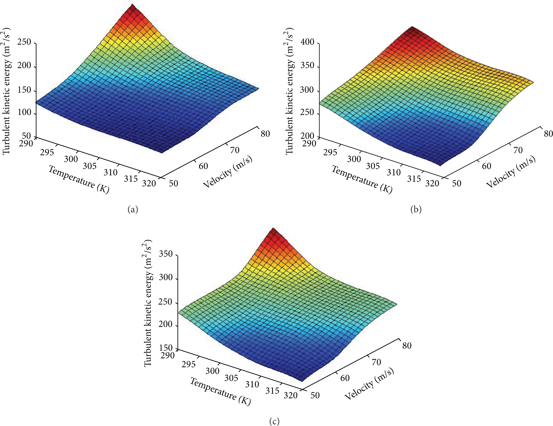
The inlet turbulent kinetic energies for different conditions of the abrasive flow polishing in a U-type tube obtained by simulation using different temperature conditions are as given in Tables 1, 2, 3, and 4 for an inlet velocity of 70 m/s. It can be observed that the turbulent kinetic energy varies with the temperature in each section of the tube. Furthermore, using different inlet velocities of 50, 60, and 80 m/s, the relationship between the temperature and the turbulent kinetic energy for each section of the tube was obtained as shown in Figure 12. Figures 12(a), 12(b), and 12(c), respectively, correspond to sections 1, 2, and 3.

Figure 12:

Relationship between the temperature and turbulent kinetic energy in a U-type tube ((a), (b), and (c) resp., correspond to sections 1, 2, and 3 of the tube).

It can be seen from Figure 12 that the turbulent kinetic energy increased with increasing processing temperature in each section of the tube. This was because the increasing velocity increased the turbulent kinetic energy. The turbulent flow was maximum at the corner of section 2, which indicates that the abrasive flow movement was most intense in this section, and the processing capacity was thus highest.

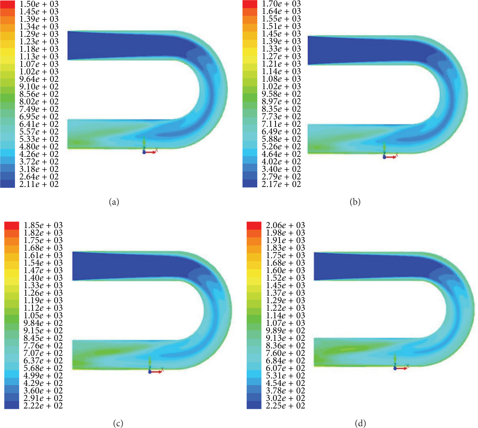
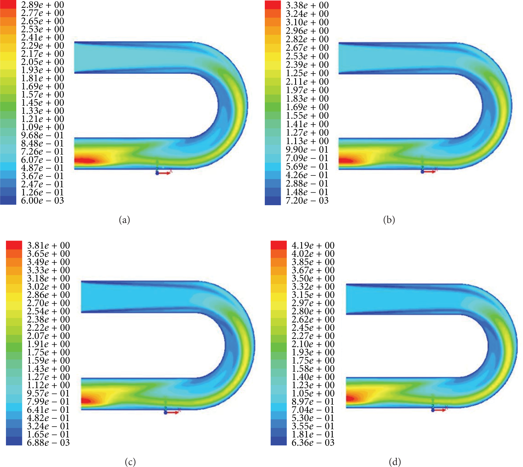
For comparison, numerical simulations of the polishing in the tube were carried out using different inlet velocities but the same inlet turbulent kinetic energy of 9.375 m²/s² and temperature of 300 K. The turbulent kinetic energy, turbulence intensity, turbulent viscosity, and dynamic pressure were determined. The results are shown in Figures 13 to 16, where (a), (b), (c), and (d), respectively, correspond to velocities of 50, 60, 70, and 80 m/s.

Figure 13:

Turbulent kinetic energy cloud in U-type tube channel for different velocities.

Figures 13 and 14, respectively, show the turbulent kinetic energy and turbulence intensity in the U-type tube for different velocities. As can be seen, the turbulent kinetic energies and turbulence intensities near the wall of the tube, at the inlet, near the bend, and at the outlet all increased with increasing inlet velocity, and the values were maximum at the bend of the tube, which indicates that the abrasion of the grains was more intense at the bend.

Figure 14:

Turbulence intensity image of U-type tube channel for different velocities.

It can be seen from the turbulent viscosity images in Figure 15 that the turbulent viscosity near the wall of the U-tube in section 1 was lower than that at the center.

Figure 15:

Turbulent viscosity cloud in U-type tube channel for different velocities.

Figure 16:

Dynamic pressure nephrogram of U-type tube channel for different velocities.

Figure 16 shows that the dynamic pressure near the wall of the tube increased with increasing velocity, although the increase was not substantial. Based on the observed turbulent kinetic energies, turbulence intensities, turbulent viscosities, and dynamic pressures for the different velocities, the U-type tube channel can be divided into three sections, namely, the straight section after the inlet (section 1), the curved section (section 2), and the straight section before the outlet (section 3). By in-depth comparative analyses of the different parameters for the different inlet velocities using an inlet temperature of 300 K and inlet turbulent kinetic energy of 9.375 m²/s², the turbulent kinetic energy and turbulence intensity distributions presented in Table 5 were obtained.

Table 5:

Distributions of turbulent kinetic energy and turbulence intensity in U-type tube channel for inlet temperature of 300 K and turbulent kinetic energy of 9.375 m²/s².

Velocity (m/s)	Turbulent kinetic energy (m²/s²)			Turbulence intensity
Velocity (m/s)	section 1	section 2	section 3	section 1	section 2	section 3

50	110	235	195	1 080	1 300	1 180
60	125	255	210	1 100	1 330	1 201
70	160	290	245	1 140	1 370	1 240
80	180	315	260	1 160	1 395	1 255

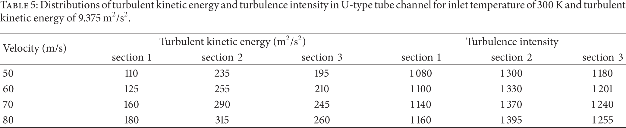
It can be seen from Table 5 that the turbulent kinetic energy and turbulence intensity in the U-type tube channel increased with increasing velocity and that the turbulent kinetic energy at the bend in the tube was relatively large. The increase in the amplitude of the turbulent kinetic energy was maximum for a velocity of 70 m/s. Moreover, the increase in the turbulent kinetic energy and the increase in the turbulence intensity between sections 1 and 2 and between sections 2 and 3 for a velocity of 60 m/s were less than those for velocities above 70 m/s. Hence, the distributions of the two parameters for an inlet velocity of 70 m/s are preferable for a U-tube channel. Table 6 gives the distributions of the turbulent viscosity and dynamic pressure in the U-type tube for an inlet temperature of 300 K and turbulent kinetic energy of 9.375 m²/s².

Table 6:

Distributions of turbulent viscosity and dynamic pressure in U-type tube channel for inlet temperature of 300 K and turbulent kinetic energy of 9.375 m²/s².

Velocity (m/s)	Turbulent viscosity (kg/m·s)			Dynamic pressure (MPa)
Velocity (m/s)	section 1	section 2	section 3	section 1	section 2	section 3

50	0.8	1.8	2.5	5	5.34	6.49
60	1.05	2	2.65	5.01	5.35	6.49
70	1.32	2.22	2.82	5.02	5.35	6.48
80	1.35	2.4	3.08	5.02	5.36	6.51

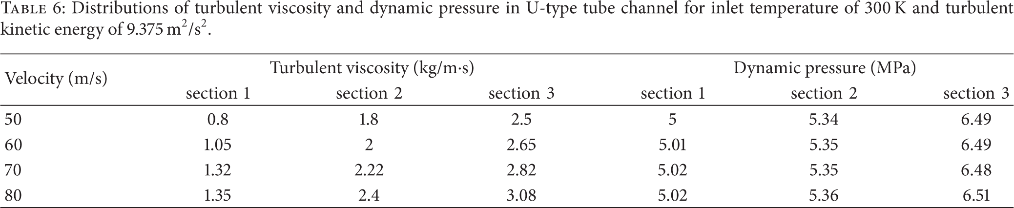
It can be seen from Table 6 that, for a high inlet velocity, the turbulent viscosity in the U-type tube initially decreases between sections 1 and 2 and then increases between sections 2 and 3. Comparative analyses revealed smaller differences in the turbulent viscosity between sections 1 and 2 and between sections 2 and 3 for an inlet velocity of 70 m/s. Comparison of the dynamic pressures in Table 6 reveals that, with increasing velocity, the dynamic pressure in the U-type tube initially decreased between sections 1 and 2 and then increased between sections 2 and 3. The turbulence viscosity and dynamic pressure distributions for a velocity of 70 m/s are thus preferable.

By simulation of a U-type tube abrasive flow polishing process using different inlet turbulent kinetic energies and velocities, the data in Tables 1, 2, 5, and 6 were obtained and were used to determine the relationship between the velocity and the turbulent kinetic energy in each section of the tube for an initial temperature of 300 K. Corresponding relationships were obtained for initial temperatures of 290, 310, and 320 K. Figures 17(a), 17(b), and 17(c), respectively, show the relationships for sections 1, 2, and 3.

Figure 17:

Relationship between velocity and turbulent kinetic energy in U-type tube ((a), (b), and (c) respectively show the relationships for sections 1, 2, and 3).

Figure 17 shows that during the process of the abrasive flow polishing in the U-type tube, the process velocity increased, the turbulent kinetic energy in each section of the tube increased, and the temperature of each section decreased. As can be seen from Figure 18, the turbulent flow was maximum in section 2. This was because the abrasive flow changed suddenly by collision of the grains with the tube wall, which resulted in increased turbulent kinetic energy.

Figure 18:

Relationship between temperature and velocity during abrasive flow polishing in U-type tube.

The results of the simulation of the U-type tube abrasive flow polishing using different temperature and velocity conditions were compared and analyzed based on the data in Tables 3, 4, 5, and 6. An inlet turbulent kinetic energy of 9.375 m²/s², a process velocity of 70 m/s, and an initial temperature of 300 K were used to determine the best distributions of the near-wall turbulent kinetic energy, turbulence intensity, turbulent viscosity, and dynamic pressure. Initial temperatures of 290, 310, and 320 K were similarly used for the simulation, and the relationship between the abrasive flow polishing temperature and velocity was determined. Inlet turbulent kinetic energies of 3.375 and 13.5 m²/s² were further used for the simulation and the corresponding relationships were obtained. The obtained relationships are shown in Figure 18. As can be seen from the figure, the process velocity gradually increased with increasing temperature, but the rate of increase began to reduce after attainment of a particular temperature. At this point, the abrasive flow machining velocity also almost ceased to increase. This was because the abrasive flow fluid viscosity in the tube decreased with decreasing temperature. There was no obvious effect of the velocity change near the wall on the process.

5. Conclusion

In this study, we investigated abrasive flow polishing in a U-type tube by an analysis of the thermodynamic energy balance equation of the two-phase solid-liquid flow. The flow and heat transfer characteristics were examined by numerical simulation, and the effects of the turbulent kinetic energy, turbulence intensity, turbulent viscosity, and dynamic pressure on the quality of the polishing process were examined to establish the theory of the process.

Using different inlet conditions for the simulation, the turbulent kinetic energies for different temperatures were analyzed, and the relationships between the temperature and the turbulent kinetic energy in the different sections of the U-type tube during the abrasive flow polishing process were obtained. By comparison of the turbulent kinetic energies for different inlet velocities, the relationships between the velocity and the turbulent kinetic energy in the different sections of the tube were also determined. Furthermore, by comparing the temperatures for different velocities, the relationships between the temperature and the velocity for different inlet turbulent kinetic energies were determined. The parameter relationships obtained in this study can be used for the optimization of the parameters of abrasive flow polishing. Based on the obtained relationship between the temperature and the velocity, the particle velocity and temperature of abrasive flow polishing in a U-type tube can be limited within an optimal range to improve the efficiency of the process and the quality of the polished surface.

Conflict of Interests

The authors declare that there is no conflict of interests regarding the publication of this paper.

Footnotes

Acknowledgments

The authors would like to thank the National Natural Science Foundation of China (no. NSFC 51206011), Jilin Province Science and Technology Development Program of Jilin Province (no. 20130522186JH), and Doctoral Fund of Ministry of Education of China (no. 20122216130001) for financially supporting this research.

References

Zheng

W.-J.

J.-Y.

, and Hao

, “Three-dimensional computer numerical simulation for micro-hole abrasive flow machining feature,” International Review on Computers and Software, vol. 7, no. 6, pp. 1283–1287, 2012.

Liu

W. N.

J. Y.

Yang

L. F.

Liu

Zhao

, and Yu

, “Design analysis and experimental study of common rail abrasive flow machining equipment,” Advanced Science Letters, vol. 5, no. 2, pp. 576–580, 2012.

Huang

Y.-Y.

Marshall

J.-E.

Carlos

G.-L.

, “Variation in carbon nanotube polymercomposite conductivity from the effects of processing, dispersion, aging and sample size,” Material Express, no. 1, pp. 315–328, 2011.

J.-Y.

Yang

L.-F.

Liu

W.-N.

, “Experimental research into technology of abrasive flow machining non-linear tube runner,” Advances in Mechanical, vol. 2014, Article ID 752353, 9 pages, 2014.

Jain

R. K.

Jain

V. K.

, and Kalra

P. K.

, “Modelling of abrasive flow machining process: a neural network approach,” Wear, vol. 231, no. 2, pp. 242–248, 1999.

Jain

R. K.

Jain

V. K.

, and Dixit

P. M.

, “Modeling of material removal and surface roughness in abrasive flow machining process,” International Journal of Machine Tools and Manufacture, vol. 39, no. 12, pp. 1903–1923, 1999.

Jain

R. K.

and Jain

V. K.

, “Optimum selection of machining conditions in abrasive flow machining using neural network,” Journal of Materials Processing Technology, vol. 108, no. 1, pp. 62–67, 2000.

Jain

R. K.

and Jain

V. K.

, “Specific energy and temperature determination in abrasive flow machining process,” International Journal of Machine Tools and Manufacture, vol. 41, no. 12, pp. 1689–1704, 2001.

Jain

R. K.

and Jain

V. K.

, “Stochastic simulation of active grain density in abrasive flow machining,” Journal of Materials Processing Technology, vol. 152, no. 1, pp. 17–22, 2004.

10.

Sankar

M. R.

Jain

V. K.

, and Ramkumar

, “Rotational abrasive flow finishing (R-AFF) process and its effects on finished surface topography,” International Journal of Machine Tools and Manufacture, vol. 50, no. 7, pp. 637–650, 2010.

11.

Sankar

M. R.

Jain

V. K.

Ramkumar

, and Joshi

Y. M.

, “Rheological characterization of styrene-butadiene based medium and its finishing performance using rotational abrasive flow finishing process,” International Journal of Machine Tools and Manufacture, vol. 51, no. 12, pp. 947–957, 2011.

12.

Sankar

M. R.

Jain

V. K.

, and Ramkumar

, “Experimental investigations into rotating workpiece abrasive flow finishing,” Wear, vol. 267, no. 1–4, pp. 43–51, 2009.

13.

Furumoto

Ueda

Amino

, and Hosokawa

, “A study of internal face finishing of the cooling channel in injection mold with free abrasive grains,” Journal of Materials Processing Technology, vol. 211, no. 11, pp. 1742–1748, 2011.

14.

Kar

K. K.

Ravikumar

N. L.

Tailor

P. B.

Ramkumar

, and Sathiyamoorthy

, “Performance evaluation and rheological characterization of newly developed butyl rubber based media for abrasive flow machining process,” Journal of Materials Processing Technology, vol. 209, no. 4, pp. 2212–2221, 2009.

15.

S.-M.

C.-H.

Tan

D.-P.

Yuan

Chi

, and Zhao

, “Study on machinability of softness abrasive flow based on preston equation,” Journal of Mechanical Engineering, vol. 47, no. 17, pp. 156–163, 2011.

16.

S. M.

Tang

Tan

Gong

Yuan

, and Pan

, “Structured surface softness abrasive flow precision finish machining and its abrasive flow dynamic numerical analysis,” Journal of Mechanical Engineering, vol. 46, no. 15, pp. 178–184, 2010.

17.

Wan

Ang

Y. J.

, and Sato

, “Development of a material model for visco-elastic abrasive medium in Abrasive Flow Machining,” in Proceedings of the 14th CIRP Conference on Modeling of Machining Operations, pp. 351–356, 2013.

18.

Wang

A. C.

Tsai

Liang

K. Z.

Liu

, and Weng

, “Uniform surface polished method of complex holes in abrasive flow machining,” Transactions of Nonferrous Metals Society of China, vol. 19, no. 1, pp. s250–s257, 2009.

Numerical Thermodynamic Analysis of Two-Phase Solid-Liquid Abrasive Flow Polishing in U-Type Tube

Abstract

1. Introduction

2. Numerical Thermodynamic Model of Two-Phase Solid-Liquid Flow

2.1. Energy Conservation Equation

2.2. Particle Temperature Equation

3. Development of Physical Model of U-Type Tube

3.1. Energy Conservation Equation

3.2. Energy Conservation Equation

4. Results and Discussion

5. Conclusion

Conflict of Interests

Footnotes

Acknowledgments

References