
Abstract
Simultaneous heat and mass transfer are investigated in a falling film outside grooved and smooth tubes. A numerical analysis of the helically trapezoidal-grooved and reference smooth tube was performed in the computational fluid dynamics program “Ansys Fluent 14.” The three-dimensional model drawings in the x, y, and z coordinates are used, and the effects of the falling film outside the helically grooved tube on the surface temperature and surface heat transfer coefficient are determined. The average surface temperature, heat transfer coefficient, and Nu values are determined experimentally for a constant heat flux. An uncertainty analysis and Nu correlation for the grooved tube are also provided in this study. The Reynolds number varied between 50 and 350 for the falling film and between 1500 and 3500 for air. Using a computational fluid dynamics (CFD) analysis for the reference smooth tube, the experimental results are validated within 2–12% difference. The experimental results are also within 6–13% of the grooved tubes.
1. Introduction
The use of closed type cooling towers and evaporative condensers is becoming widespread. Increasing the wet surface area in the heat exchangers, absorbers, and evaporators in absorption cooling systems increases heat and mass transfer, thereby reducing the capital and operating cost of the system.
In the literature, the experimental results for a falling film-type flow vary according to the fluid type, tube material, and the number and order of tubes.
Rogers [1] used the integral method to analyze the energy equations for a laminar film flow falling on moving and horizontal tubes. Rogers expressed the laminar film thickness at any point as a function of the Reynolds number, Archimedes number (Ar), and angular position of the horizontal tubes.
Hu and Jacobi [2, 3] observed changes based on the separation interval in droplet and jet-type flows. Liquid film flows from one tube to another, whereas the flow forms discrete droplets, discrete jets, or a continuous sheet flow. In the experiments, effects of thermophysical properties and geometric parameters (in droplet and jet flow) were discovered and introduced. Under the conditions of that study, the departure-site spacing increases as the Reynolds number decreases for fluids with a high modified Galileo number (Ga). As with fluids with low Ga numbers, departure-site spacing is independent of Reynolds number. In small tubes, the diameter of the tube and departure-site spacing slightly increase. This increase is independent of the tube dimension in large tubes. Although departure-site spacing is independent of tube spacing, the relationship between the type of jet flow, wavelength in the jet flow, and the tube spacing was observed under several conditions.
Liu et al. [4] performed experimental and numerical studies investigating the evaporation of water films falling on horizontal tube bundles in evaporators. The heat transfer coefficients of the water film horizontally falling on heated tubes were calculated using laminar and turbulence models. The calculation area around the heated tube was divided into two parts: the stagnation zone and the lateral free film zone. This previous study found that the diameter of the tube affected the heat transfer.
Kim and Kang [5] investigated the effect of hydrophilic surface treatment on evaporative heat transfer from the outer wall surface for various copper tubes, from which smooth, spiral, corrugated, and low-finned tubes were selected as the test tubes.
Roques and Thome [6] presented the flows and transits for four types of expanded tubes. These are Wieland Gewa-K40 (40 fpi), Wieland Gewa-K19 (19 fpi), and Wolverine low fin (26 fpi and 29 fpi) tubes. Comparing these tubes with smooth tubes displays the effect of fins and fin density on the transits. The basic finding was that a high fin density (40 fpi) does not affect the transit significantly when compared with smooth tube transits. However, low fin densities (29 fpi and 26 fpi) increase the Reynolds number of the transits.
Louahlia-Gualous et al. [7] presented numerical results for reverse heat transfer and experimental results for local heat transfer in falling films. These authors found that the local heat transfer coefficients increased as the air speed and flow rate of a liquid film increased or as the temperature of an input film decreased. Correlations were developed for the mean heat transfer coefficients in the stagnation region, the thermally developed region, and the lower side of the heated cylinder.
A study performed by Ribatski and Jacobi [8] summarized the existing literature on horizontal type falling film-type evaporators. That study also examined a single smooth tube, enhanced surfaces, and the flow model that affects heat transfer on tube bundles and experimental parameters.
Jafar et al. [9] studied the effects of the liquid flow field on the Reynolds number, cylinder diameter, and the spatial placement of the cylinder in droplet mode. The range of the Reynolds number in that study was 50 to 2000. A finite-volume finite-difference computational fluid dynamics (CFD) code, FLUENT, was used in their simulations. The volume of fluid (VOF) technique has been employed to mark a point occupied by fluid as unity and a point occupied by air as zero.
Additionally, Jafar et al. [10] determined the behavior of a liquid film flow over horizontal cylinders. That study employed a CFD code in Fluent for 2D configurations with one, two, and three cylinders.
Luo et al. [11] studied the two-dimensional CFD of a falling film evaporating from horizontal tubes with different shapes during seawater desalination. The flow and heat transfer characteristics of the falling water film on one circular tube and two noncircular shaped tubes (drop-shaped and an oval-shaped) were analyzed. They found that the average heat transfer coefficients of the oval- and drop-shaped tubes were approximately 34.03% and 12.63% higher than those of the circular tube, respectively, with a mass flow rate of 0.49 kg/m·s and a spray height of 0.009 m.
It is important to determine the heat transfer coefficient in simultaneous heat and mass transfer mechanism. Unlike other studies, different groove geometries are investigated by the computational fluid dynamics program “Ansys Fluent 14,” and heat transfer coefficients were found for different conditions. The geometry of the groove was designed, and the results of the analysis are compared with experimental results. Furthermore, this study determines the heat transfer coefficient during evaporation. The surface temperature is set to a constant value for a heated tube, and a falling film is investigated in different conditions.
2. Experimentation
A schematic illustration of the experimental system is presented in Figure 1. In the experimental system, thermocouples, hygrometers, anemometers, and flowmeters were employed as measuring equipment [12]. The system also contains a test cabinet, feeding unit, radial fan, air duct, power source, proportional-integral-derivative (PID) controller unit, frequency changer, VTI ex1200 series multichannel data recorder, and heating elements.

Schematic illustration of the experimental system.
Measurements were conducted at 9 points along the test tube—3 points up to the tenth, twentieth, and thirtieth centimeter and 3 points circumferentially (Figure 2). To provide a uniform surface temperature in the axial direction, the test tubes were copper, and the walls were 3 mm thick. Three notches were formed at equal spacings on the surface in the axial direction. Thermocouples can be partially buried in these notches. To determine the circumferential temperature distribution, two additional notches were formed at 90° angles. The circumferential thermocouples were fixed on the surface using a thin fishline to hold the three thermocouples along the same vertical and horizontal axes. Heat emery paste was applied to the thermocouples. The thermocouples can be affixed between the pitches according to the groove geometry by using the identical method. Among the 9 thermocouples employed, the average of the longitudinal thermocouples assists the determination of the temperature of the upper surface, the temperature of the side surface, and the temperature of the bottom surface of the tube. The test cell, test tube (outer diameter of 18 mm) (helically trapezoid grooved type), and the groove's geometric features are depicted in Figure 2.

(a) Schematic of the test cell and (b) properties of grooved tube.
A numerical analysis of the helically trapezoidal-groove and reference smooth tube was performed in the computational fluid dynamics program “Ansys Fluent 14.” After the necessary definitions were provided in the Ansys 14 workspace, the model was constructed with the “Design Model” program. A mesh design for the model drawn was performed by the program “Mesh Modeler.” SIMPLE (semi-implicit methods for pressure linked equations) were employed to solve for the correlation between the pressure and velocity in the numerical analysis. This method is a convenient method for steady flows.
Under forced convection conditions, the order of operations performed in the experiments with both grooved tube and reference smooth tube is shown in Figure 3.

Flowchart depicting the experimental operations.
The tube surface temperature, which has a uniform temperature distribution, was provided by a silicone coated electric heater. The voltage of the power supply was measured with a multimeter for the tube heater and was recorded for each experiment. Experiments are started after the surface temperature was constant. The experiments were followed by a written program in the DAC Express software.
3. Control of the Mesh System
During the creation of meshing grids in the ANSYS ICEM CFD program, setting the meshing as frequent or loose depends on the user. The number of meshing grids is important for the accuracy of the solution. Therefore, the number of meshing grids must be accurately determined. In this study, a thinning mesh is preferred in the y direction and a frequent mesh in the z direction to determine the effects of the flow outside the three-dimensional grooved tube and the tube surface boundary layer. The meshing along the surface of the tube and along the imaginary plane perpendicular was placed at different intervals. The meshing sections alter from 5, 10, 15, 20, 25, 30, 35, 40, 45, 50, 100, and 500 for the imaginary plane (specified with yellow color in Figures 4 and 5). Along the tube surface, the meshing was produced from 283 to 28,300 units of area. Five-sectional meshings on the tube surface can be seen in Figure 4, and fifty-sectional meshings on the tube surface can be seen in Figure 5.
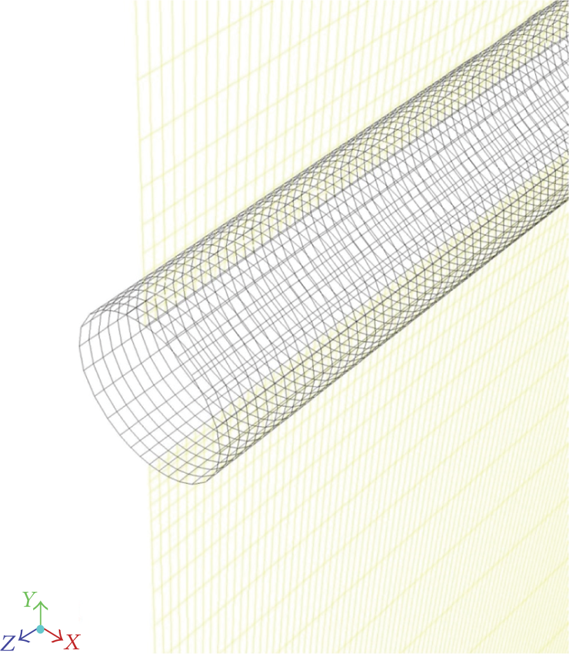
Meshing grid (five-sectional) on the tube surface.

Meshing grid (fifty-sectional) on the tube surface.
The h values, surface temperature values, and Nu values calculated by the Fluent program for the smooth tube are listed in Table 1.
Determining the meshing grid for the reference smooth tube.

3.1. Grooved Model Drawing and Meshing
A three-dimensional model was drawn in the “Design Modeler” program for the grooved tube and the reference smooth tube. The program cannot calculate two-dimensional drawings (x and y coordinates) because the groove structure changes according to the width of the groove in the z coordinate. Therefore, three-dimensional model drawings in the x, y, and z coordinates were used, and the effects of the falling film outside the helically groove tube on the surface temperature and surface heat transfer coefficient were determined. A helically trapezoidal-grooved tube model that was drawn by “Design Modeler” and the selected meshing grid can be seen in Figure 6.

(a) Helically trapezoidal-grooved tube model and (b) meshing grid used.
For the numerical analysis in the tube around the boundary layer and the tube outer surface, the reference smooth tube, and the imaginary axis plane along the common flow in the test cell at the outlet, the mesh is sparse and arranged.
In this numerical study, a grooved tube surface boundary layer and the outside surface of the tube were observed; therefore, a frequent mesh was preferred along the imaginary plane and a thinning mesh was preferred in the inlet and outlet of the test cell (the mesh was identical in the reference smooth tube).
3.2. Residual Results
The analysis for the reference tube was terminated after 2000 iterations within 3 hours for the ten-sectional grid. The convergence curve flattens after 6000 iterations (Figure 7). A solution in the grooved tube was achieved after 5000 iterations within 6 hours (Figure 8).

Residual values in the reference tube analysis.

Residual values in the grooved tube analysis.
4. Theoretical Analysis
The heat convection coefficient with Newton's cooling law is defined in

where h d is the heat convection coefficient for the case of air flow on the test tube and A c represents the total surface area in contact with the fluid and is calculated using a computational model for a grooved tube. Neglecting the heat transferring from the tube surface via radiation, the thermodynamic energy balance according to the first law of thermodynamics is expressed by

where Q c is the heat transfer with convection and Q h is the heat flow given to the system by an electrical heater:

By combining (1), (2), and (3), the heat convection coefficient (h d ) is determined by (4) where U is the voltage value applied to the electrical heater from the power source (V) and R is the resistance value (Ohm) of the in-tube heater:

The Nusselt number was calculated using the calculated convective heat transfer coefficients:

where k a is the thermal conductivity (W/m2·K) of the air. The falling water film flows from the tube surface with different water flow rates, and the experiments were also conducted under different forced convection conditions. The air viscosity, heat transmission coefficient, and thermophysical properties (such as α, μ, and Pr) were calculated using the film temperature; the evaporation latent heat (h fg ) was calculated using the surface temperature. The film temperature is defined by

The experiments were performed under different forced convection conditions. The control volume is shown in Figure 2. For the test cell, the total heat transfer according to the first law of thermodynamics is as follows:

When the equation is rearranged,

where i represents the lower index input and o represents the lower index output:

When (8) and (9) are combined,

The flow rate of evaporating water is

The flow rate of evaporating water was determined using (12) based on experimental measurements:

where V is the speed (m/s) and A is the cross-sectional area vertical to the flow of the test cell (m2). The absolute humidity at the input and output of the test cell was calculated using (13) based on measurements of relative humidity and temperature using a hygrometer:

In this study, the water film flowing from the upper side and the heat and mass transfer in air occur simultaneously. Furthermore, the total heat transfer between these two flows is the total of the sensible and latent heat transfer. When heat transfer with convection is expressed by rewriting the energy balance according to the thermodynamic first law, the following equation occurs:

Radiation heat transfer is neglected because the experiments are performed under forced convection conditions. The transfer of sensible heat occurs because of the temperature difference between the water drops and air. A humidity-saturated air layer emerges in the region defined as the “interface” and upon the water film surface. The partial pressure of the water vapor is larger than the partial vapor pressure of the water vapor within the free air flow. Therefore, mass transfer occurs because of the water vapor evaporating from the water film surface and transferring into the air. Depending on the concentration difference of the amount of evaporating water, the mass transfer is expressed as follows:

According to the Chilton-Colburn equality [13],

where n can be taken as 1/3. The Le number is determined using

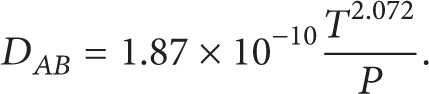
The program Refprop v7.0 was used to determine certain physical properties. D AB is the diffusion coefficient and is calculated using the following formula:
When (16) and (17) are combined, the heat convection coefficient is determined using (18) depending on the Chilton-Colburn equality:

Under forced convection conditions, the heat transfer is proportional to the temperature difference. When convection is defined according to the Newton cooling law, the heat flow is defined as (19):

The Nusselt number is calculated using

Equation (22) describes the heat transfer coefficient of a falling water film:

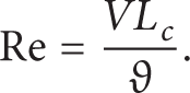
The Reynolds value is determined for the air side using
The Reynolds number of the falling water films is defined using [12]

Equation (25) determines the hydraulic diameter of the water film falling from the outer surface of the tube:

The Reynolds number of the falling water films is determined based on the groove geometry. When the definition of the hydraulic diameter and the Reynolds equality are combined, the following is found:

The geometric properties of the helically trapezoid grooved tube are presented in Figure 9.

Properties of a helically trapezoid groove.
The wet circumference for the grooved tube is calculated using

The area of the helically trapezoid grooved tube is calculated using [14]

Therefore, the following can be written:

5. Experimental Results
The measurements taken without generating a falling film-type flow under forced convection conditions in a reference smooth tube were compared to the results in the literature. As displayed in Figure 10 in the percentage error columns, the Nusselt number, with an error rate of ±11%, includes the correlation results of [15–17].
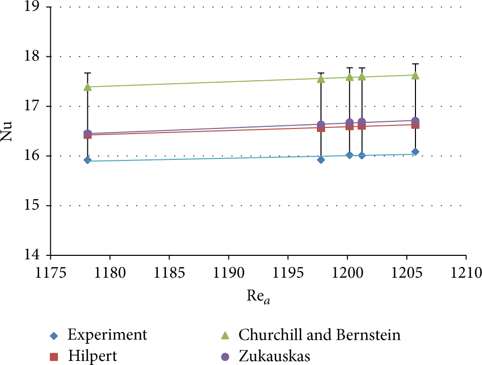
Comparison of Nu values under forced convection conditions in a reference smooth tube (T s = 40°C).
Heat and mass transfer occur simultaneously in all experiments; therefore the amount of evaporation from the water film falling from the surface of the grooved tube was examined in the experiments at a constant surface and feeding water temperature. The amount of evaporating water increased with increasing the flow rates of the feeding water (Figure 11).

Amount of water evaporating under different temperatures in a grooved tube (v a = 1.5 m/s).
The two drawings of the tube geometry are read by the Fluent program, and identical boundary conditions are used. The average surface temperature, heat transfer coefficient, and Nu values are determined experimentally in the constant heat flux process, and they are listed in Table 2.
Numerical and experimental results for the reference smooth tube and grooved tube.

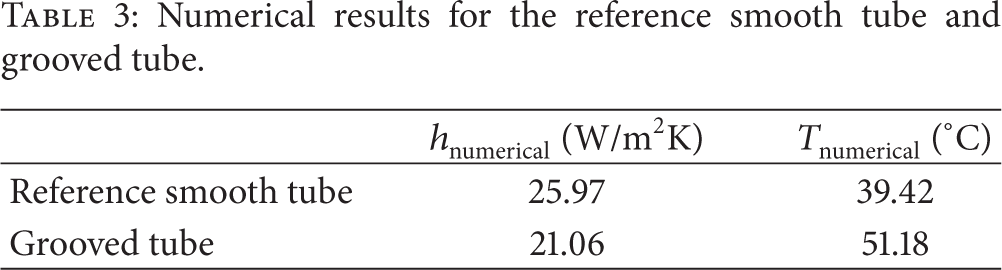
The numerical analysis results calculated by Fluent are given in Table 2, and the difference between these values and the experimental results are shown. Also the surface heat transfer coefficient is determined with the help of the Fluent program for the identical conditions. The results are given in Table 3.
Numerical results for the reference smooth tube and grooved tube.
The ratio of the flow rate of evaporating water to the flow rate of feeding water and a comparison figure of the grooved tube and reference smooth tube are shown in Figure 12. The rate of evaporation is approximately 25% lower in the reference smooth tube than in the grooved tube.

The rate of evaporation in the reference smooth tube and grooved tube (Tfe = 35°C).
The values from other studies in the literature were compared to the values of hff (W/m2K) convection coefficient that was determined for a falling water film. The convection coefficient values of a falling water film found under identical conditions using correlations of [18, 19] are shown in Figure 13.

Comparison of Nu numbers determined for a falling water film with the literature.
A comparison of the heat convection coefficients determined experimentally with the heat convection coefficients calculated with Colburn simulations of experimental findings is shown in Figure 14. The experimental results of the Colburn equation approximated for nearly ±5% of the actual results.

Comparison of Colburn equality with experimental results.
The general Nu equation depends on variables such as the Re number, Prandtl number of air and, the Re number of the water films. This equation is expressed as Nu g = f (Pr,Re a ,Re w ). The correlation is determined with the equation below with a constant a of 1.9778, constant b of 0.15646, and constant c of 0.73441:

The operation interval of this correlation is detailed in Table 4 depending on Tfe temperature, Re w , and Re a .
Operation interval of the Nu correlation.
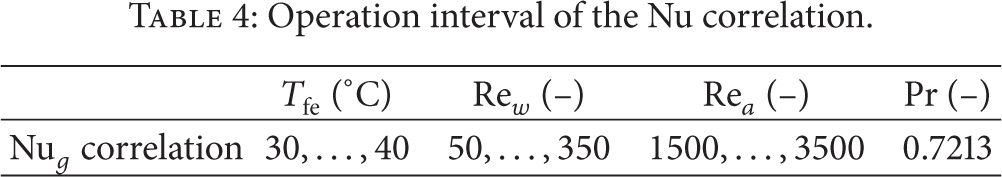
The numerical values of the correlation and experimental results were compared, and ±25% accuracy was observed (Figure 15).

Error analysis of the grooved tube correlation (Nu).
5.1. Analysis of Uncertainty
The accuracy of the experimental results is affected by the measurement devices and the errors resulting from the experimental setup. Several methods have been recommended to determine the error ratios pertaining to parameters that are calculated using the data obtained from experiments. The uncertainty analysis method developed by Kline and McClintock [20] for the error analysis of experimental findings is one such method. For the error analysis conducted for this experimental study, the uncertainty analysis method was more sensitive than other methods.
If the error rates of each independent variable are w1,w2,w3,…,w n and the error rate of the magnitude of C is w c , then the uncertainty is expressed as follows according to the analysis of uncertainty:
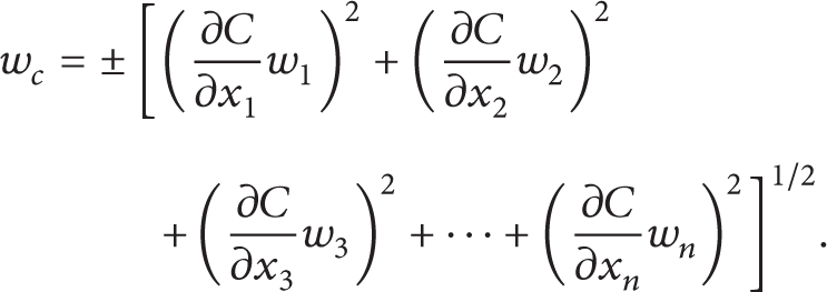
Because the heat and mass transfer occur simultaneously, the uncertainties were observed to result from the experimental measurements for the heat convection coefficient (h c ) and heat convection coefficient of the falling water film flow (hff) in the air-water interface because of the measurement of independent variables such as the relative humidity (φ), temperatures of the tube surface (T2, T3, T4, T5, T6, T7, T8, T9, and T10), and the heater power (Q). The accuracies of the instruments used in the experiments are listed in Table 5.
Experimental accuracy.

Equation (32) expresses h c to determine the uncertainty of the convection coefficient:

The uncertainty value is expressed as follows:

Equation (34) describes the energy balance and performs an error analysis:


The convection coefficient of the falling water film is calculated using


Furthermore, the uncertainty analysis was also performed for the nondimensional parameters determined as a Nusselt number. The error rate of the Nusselt number is the following:
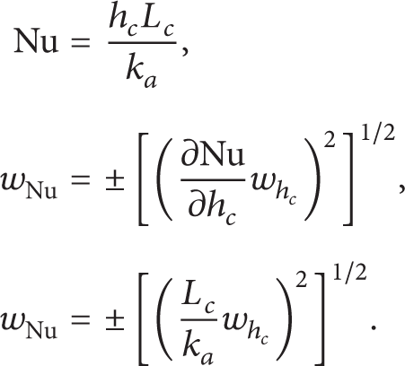
The results of the uncertainty analysis of the experimental results are presented in Table 6.
Uncertainty values of the experiments on the grooved tubes and reference smooth tubes.

6. Results and Conclusions
In this study, a smooth tube and grooved tube in forced convection conditions were studied to determine their heat transfer performance. A CFD analysis was performed on both tube types. The evaporation at different temperatures was also experimentally investigated. The testing apparatus was validated with the results of the CFD analysis and the literature. Numerical and experimental results are listed below for the falling film outside the helically grooved tube and smooth tube.
In the experiments performed under forced convection conditions without a falling film-type flow for the grooved tube and the reference smooth tube, the heat convection coefficient and Nusselt numbers conform to those with error rates of ±5% of Hilpert and ±6% of Zukauskas.
As a result of the CFD analysis of the reference smooth tube, experimental results were validated with numerical results within 2–12%. Experimental results were also verified by the 6–13% difference for the grooved tubes.
The experiments were performed for a feeding water flow rate of 50–220 L/h. The amount of evaporating water increased with increasing flow rates of the feeding water. For the helically trapezoid groove geometry tube, the amount of evaporating water changes between 0.3 and 1 kg/h depending on Re w and Re a .
The effect of air speed on the amount of evaporating water was examined. According to the experimental findings, the amount of evaporating water increased as the Reynolds number of the air increased.
As the general Nusselt expression for the grooved tube, a
In falling film-type flow, the Nusselt number change was provided for the reference smooth tube and the grooved tube depending on the Reynolds number of the water films. For a constant heat flux, the grooved tube has lower heat convection coefficients than the reference smooth tube because the difference between the input temperature of the feeding water and the surface temperature of the tube was higher.
The average surface temperatures were determined for the reference and helically grooved tubes for constant heat flux conditions. As a result of the CFD analysis, the heat transfer coefficient for the grooved tube is 18% less than the heat transfer coefficient for the reference tube for only air flow.
The experimental studies performed under different air speeds and water flow rates can be used as guides in designing falling film-type flow systems. A system can be designed using the given general Nusselt correlation for desired conditions. Existing systems can operate with lower water flow rates when using a grooved geometry, and the design of more efficient devices will be possible as the surface of heat transfer is increased. In addition to this study, a CFD analysis can be performed for the evaporation from the grooved tube surface.
Footnotes
Nomenclature
Conflict of Interests
The authors declare that there is no conflict of interests regarding the publication of this paper.