Sage Journals: Discover world-class research

Abstract

With the advancements in computing power, computational fluid dynamics (CFD) analysis has emerged as a powerful hydraulics design tool. This study aims to assess the performance of CFD via commercially available software (FLOW-3D) in the prediction of backwater surface profiles for three different types of bridges with or without piers in a compound channel. A standard two-equation turbulence model (k-ε) was used to capture turbulent eddy motion. The numerical model results were compared with the available experimental data and the comparisons indicate that the CFD model provides reasonably good description of backwater surface profiles upstream of the bridges. Notably, the computed and measured afflux values are found to be almost identical.

1. Introduction

Accurate estimation of flow characteristics at and around bridge locations is main concern for the bridge engineers both in terms of stability of bridge itself and the problems caused by insufficient hydraulic design of it such as flooding due to the sudden increase in water level upstream. Depending on the flow situation, estimation of these characteristics can be difficult. Flow in a compound channel is an example of such flow situation as there is a strong transfer of longitudinal momentum from the fast moving flow in the main channel to the slow-moving flow in the floodplain. This transfer is more pronounced at the interface between the floodplain and the main channel [1]. The complexity of flow can increase by placing hydraulic structures such as abutments and piers, which block the part of flow area. In such conditions, rapidly varied flow develops near the structures due to the presence of the obstruction. Consequently, the flow is separated downstream of the structure and a reverse flow and an adverse pressure gradient occur. The water surface upstream of the structure increases and forms a backwater profile (Figure 1). A jet is generally established in the bridge opening and continues into the region of expansion immediately downstream of the bridge, where there is a strong turbulent diffusion and mixing as well as a large amount of energy losses [2]. In the case of a bridge pier, occurrences of a horseshoe vortex in front of the pier and lee-wake vortices behind it increase the complexity and are very important for the scour and scour protection studies [3]. Similar flow pattern can be observed for the bridge abutments [4, 5]. Development of scour has to be well understood by bridge engineers as most of the bridge failures occur due to the local scour, which is highly correlated with the flow processes, around bridge piers and abutments [3, 6 –8]. Moreover, a significant amount of problems caused by bridge constructions is corresponding to the backwater. It is essential to estimate the increase in the water surface level due to bridge constrictions especially in flood conditions. Maximum backwater height called afflux is also one of the key parameters in bridge design (Figure 1). This study involves the numerical prediction of backwater surface profiles in a compound channel with a bridge, which includes the previously described complexities.

Figure 1:

Definition sketch of flow through a bridge constriction.

Johnson et al. [9] pointed out that bridge piers, bridge abutments, and roadway embankments all create local obstructions that cause the flow to become highly three-dimensional. In fact, it is believed that any vertical obstruction in a channel makes formerly unidirectional flow become highly three-dimensional [10, 11]. Biglari and Sturm [2] have also recommended using 3D model in order to capture the local flow characteristics causing local scour around bridge abutments.

One-dimensional numerical models have been widely used for prediction of water surface profile around bridges such as HEC2, HECRAS, ISIS, and MIKE11 [12 –15]. Alternatively, Mantz and Benn [16] developed two one-dimensional analytical models, namely, Afflux Estimator (AE) for more detailed analysis of the water surface profiles and Afflux Advisor (AA) for the rapid estimate of the afflux rating. They verified their models with the experimental data used in this study and a large-scale field data.

In current work, the use of one-dimensional numerical models for the prediction of flow characteristics is not an option as the assumptions made in their developments are obviously violated in such complicated flow patterns although they are still the primary tool used for the river engineers. Two-dimensional numerical models for free surface flows have limited applications as they can capture the flow separation around the obstacle. Moreover, it has been shown that recently developed two-dimensional numerical models are able to simulate many types of flows including rapidly varying and discontinuous flows [17, 18]. However, they do not capture the turbulent diffusion and mixing. Biglari and Sturm [2] introduced a 2D depth averaged, k-ε turbulence model for open channel flow around bridge abutments on the floodplain in a two-stage channel. However, they also highlighted the need for further investigation of the effect of compound channel on the flow characteristics in the region close to the obstruction that requires 3D study.

Hence, FLOW-3D software [19] was selected because the previous studies indicated that flow around a bridge as well as in a compound channel show significant 3D characteristics, and it was also suggested to be a powerful hydraulic engineering design tool in modeling three-dimensional free surface flow around water structures [20 –23].

This study is an assessment and comparison of the performance of RANS based numerical model for the prediction of backwater surface profiles and afflux values in a compound channel with three different types of bridges with or without piers. The performance of the model has been tested using a wide range of experimental data, presented also in several previously published works [24, 25] obtained from series of experiments which were carried out at the Hydraulic Laboratory of Birmingham University in UK.

2. Experimental Work

Comprehensive experimental data [24, 25] regarding the measurement of flow characteristics around a bridge which had been produced in a symmetrical compound channel flume at the Hydraulic Laboratory of the University of Birmingham were used to test numerical simulations. The channel has a 22 m length, 1.213 m width, 0.4 m depth, and 2.024 × 10⁻³ bed slope. The compound channel consists of a main channel, 0.398 m in width, and two symmetric floodplains, 0.4073 m in width (Figure 2). All channel boundaries were smooth and they were constructed from PVC material. The bridges with 0.1 m width were made of polished wood.

Figure 2:

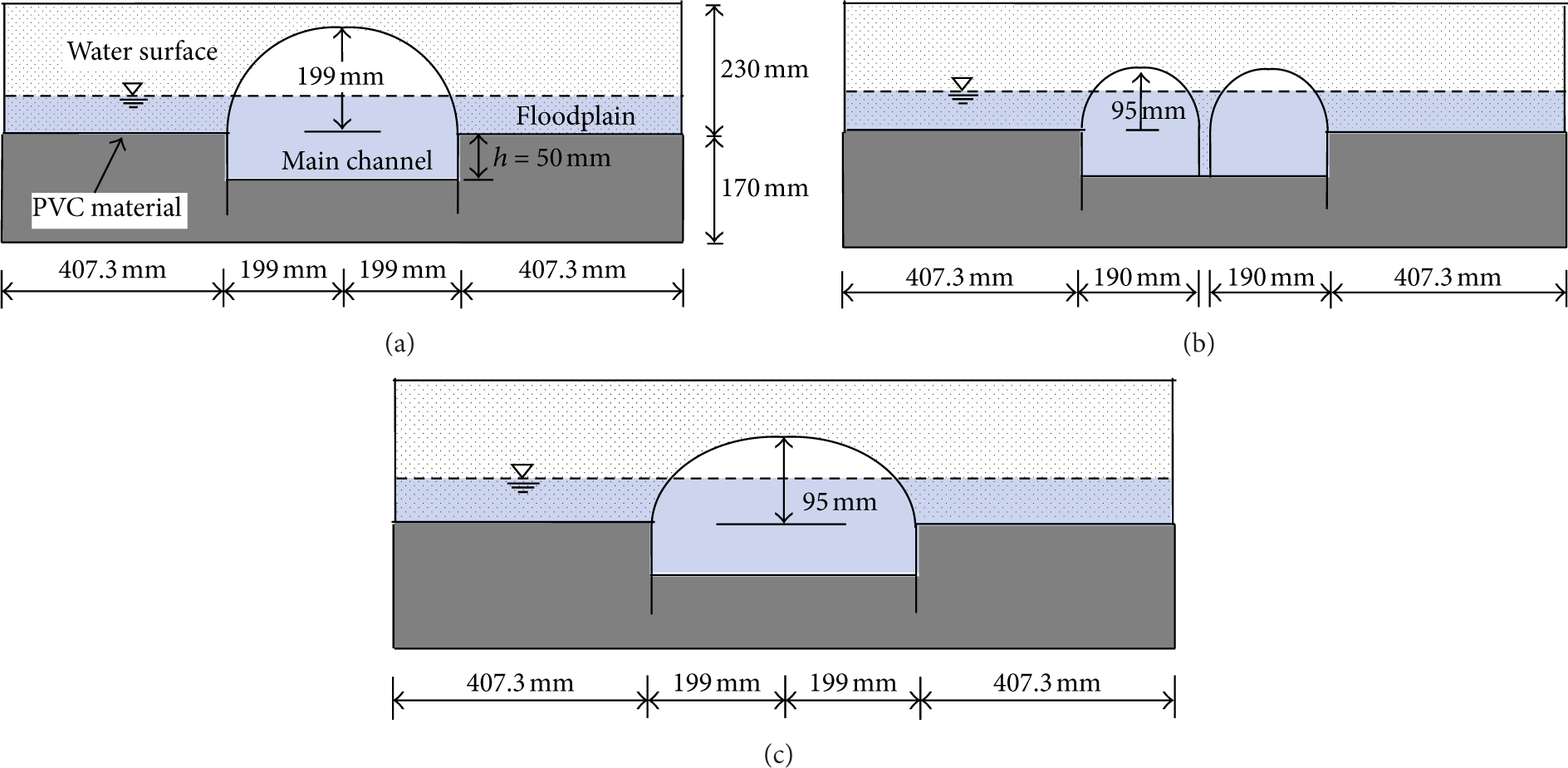
Cross-sections of bridge models used in this study: (a) single opening semicircular arch bridge model (ASOSC), (b) multiple opening semicircular arch bridge model (AMOSC), and (c) single opening elliptic arch bridge model (ASOE).

The experiments were conducted with flow rates ranging from 21 × 10⁻³m³/s to 35 × 10⁻³m³/s and the uniform water depths ranged from 60 mm to 85 mm. The tailgates at the downstream end of the flume were adjusted to produce subcritical uniform flow conditions without a bridge in the 18 m test length.

The water depths at 1 m intervals down the length of the flume were measured directly using pointer gauges with an accuracy of 0.1 mm. The readings of flow depth were then used to calculate the related flow depth. However, the water surface profiles immediately upstream of the bridges within 1 m range were measured in detail at 0.1 m intervals.

The data and a full description of the methodology are contained in two technical papers presented to JBA Consulting Engineers & Scientists and the Environment Agency (EA), as part of project titled “Scoping Study into Hydraulic Performance of Bridges and other Structures, including Effects of Blockages, at High Flows (Bridge Afflux Experiments in Compound Channels)” [24, 25]. These experimental data have also been analyzed by different researchers [16, 26].

JBA Consulting also produced two main outputs within this research program. One is Afflux Advisor (AA), which is an accessible stand-alone tool in spreadsheet form and the other is the Afflux Estimation System (AES) which is a more rigorous modeling tool with calculation of afflux based on hydraulic theory [27, 28].

The laboratory work included a total of 145 afflux measurements for bridge types of single opening semicircular arch bridge model (ASOSC), multiple opening semicircular arch bridge model (AMOSC), single opening elliptic arch bridge model (ASOE), and single opening flat deck bridge model with piers (DECKP) and without piers (DECK) including different span widths. All experiments were carried out for low flow conditions where the flow does not make contact with the low chord of the bridge models. Cross-sections of all bridge types used in this study are shown in Figure 2.

In the numerical modeling, not all 145 experiments were modeled. The total of 15 runs was selected to test the numerical solution of RANS equations.

3. Numerical Model

Computational fluid dynamics (CFD) models have become well established as tools for simulation of free surface flow over a wide range of structures. The commercially available CFD program, FLOW-3D, was used in the current study. This software has been constructed for the treatment of time dependent flow problems in one, two, and three dimensions. It is claimed to be applicable to almost any type of flow processes and provides many options for the users. It has two types of time integration methods, namely, explicit and implicit solutions, and turbulence closure is achieved in five different ways: Prandtl mixing length, the one equation turbulence energy, the two-equation k-ε equation, the renormalization group (RNG), and the large eddy simulation [19].

For three-dimensional free surface flow simulation, the Reynolds-Averaged Navier-Stokes (RANS) equations are solved by the finite volume formulation on a structured staggered finite difference grid. Mesh is also automatically generated by the program after prescribing the boundaries.

Geometry specifications are independently made on a grid, which allows generation of complex obstacles. In the current study, each bridge model was implemented in the flow domain. The program evaluates the location of the flow obstacles by utilizing a cell porosity technique called the fractional area/volume obstacle representation of FAVOR method [29, 30]. In this approach, an obstacle in a mesh is represented by a volume fraction (porosity) value ranging from zero to one as the obstacle fills in the mesh. Hence, for an obstacle the following conditions are distinguished: completely solid, partly solid and fluid, completely fluid, partly fluid, or completely empty. In FLOW-3D, free surfaces are modeled with the volume-of-fluid (VOF) technique developed by Hirt and Nichols [31].

It is readily and widely accepted that the RANS equations govern the common free surface turbulent flows. The solutions methods are also well-known powerful methods. Many examples of the applications of the solutions of the RANS equations to the similar free surface turbulent flow problems can be found in the literature [20 –23, 32].

3.1. RANS Solution with k-ε Turbulence Model

For Newtonian, incompressible fluid flow, the mass and momentum equations, which constitute the RANS equations, are given as

\begin{matrix} \frac{\partial}{\partial x_{i}} (u_{i} A_{i}) = 0, \\ \frac{\partial u_{i}}{\partial t} + \frac{1}{V_{F}} (u_{j} A_{j} \frac{\partial u_{i}}{\partial x_{j}}) = - \frac{1}{ρ} \frac{\partial p}{\partial x_{i}} + G_{i} + f_{i}, \end{matrix}

(1)

where x represents the coordinate, u_i is mean velocity, A_i is fractional area open to flow in subscript direction, t represents time, V_F is fractional volume open to flow, p is pressure, ρ is fluid density, G_i represents the body accelerations, and f_i represents the viscous accelerations given as follows:

\begin{matrix} f_{i} = \frac{1}{V_{F}} [\frac{τ_{b, i}}{ρ} - \frac{\partial}{\partial x_{j}} (A_{j} S_{i j})], \\ S_{i j} = - (ν + ν_{T}) [\frac{\partial u_{i}}{\partial x_{j}} + \frac{\partial u_{j}}{\partial x_{i}}], \end{matrix}

(2)

where τ_b,i represents wall shear stress, S_ij represents the strain rate tensor, ν is the kinematic viscosity, and ν_T is the kinematic eddy viscosity.

In computational fluid dynamics, various turbulence models were used for determining turbulence viscosity, ν_T [33]. In the present computations, the standard k-ε turbulence closure was adopted [34]. In this model, turbulence eddy viscosity is computed using turbulence kinetic energy k and turbulent dissipation rate ε per unit fluid mass as follows:

ν_{T} = \frac{C_{μ} k^{2}}{ε},

(3)

where C_μ represents an empirical coefficient.

In the standard k-ε turbulence model, the values of k and ε are determined from the following two transport equations:

\frac{\partial k}{\partial t} + u_{i} \frac{\partial k}{\partial x_{i}} = \frac{\partial}{\partial x_{i}} (\frac{ν_{t}}{σ_{k}} \frac{\partial k}{\partial x_{i}}) + ν_{t} (\frac{\partial u_{i}}{\partial x_{j}} + \frac{\partial u_{j}}{\partial x_{i}}) \frac{\partial u_{i}}{\partial x_{j}} - ε,

(4a)

\frac{\partial ε}{\partial t} + u_{i} \frac{\partial ε}{\partial x_{i}} = \frac{\partial}{\partial x_{i}} (\frac{ν_{t}}{σ_{ε}} \frac{\partial ε}{\partial x_{i}}) + C_{1 ε} \frac{ε}{k} ν_{t} (\frac{\partial u_{i}}{\partial x_{j}} + \frac{\partial u_{j}}{\partial x_{i}}) \frac{\partial u_{i}}{\partial x_{j}} - C_{2 ε} \frac{ε^{2}}{k} .

(4b)

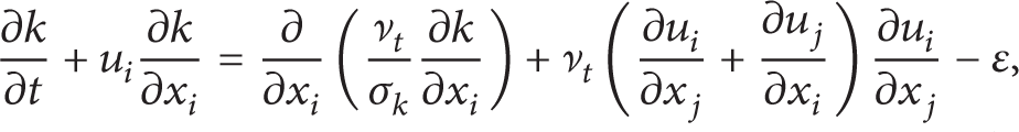
The standard values of the empirical coefficients used in the k-ε model are C_μ = 0.09, C_1ε = 1.44, C_2ε = 1.92, σ_k = 1.0, and σ_ε = 1.3.

The volume of fluid (VOF) method is used in computations of the free surface by FLOW-3D [19] in which both the water and the air are modelled in a grid. In this method, each cell has a fraction of water (F), which is 1 when the element is completely filled with water and 0 when the element is completely filled with air. If the value is between 0 and 1, the element contains free water surface. Therefore, a supplementary transport equation is added given as follows:

\frac{\partial F}{\partial t} + u \frac{\partial F}{\partial x} + v \frac{\partial F}{\partial y} + w \frac{\partial F}{\partial z} = 0,

(5)

where u, v, and w are fluid velocity components in the x, y, and z directions, respectively. The VOF method consists of three ingredients: a scheme to locate the surface, an algorithm to track the surface as a sharp interface moving through a computational grid, and a means of applying boundary conditions at the surface [31].

3.2. Solution Domain, Boundary, and Initial Conditions

Prior to computation, the computational domain, 18 m long, was divided into structured grids and boundary and initial conditions were prescribed. As shown in Figure 3(b), only the half of the computational domain (60.63 cm) along the channel was taken into account both in the construction of grids and the simulation due to the symmetry. The height of the computational domain was set ranging from 20 to 23 cm depending on the initial flow depth in the channel. The channel bottom slope is set to be 0.002024.

Figure 3:

Computational domain and boundary conditions: (a) longitudinal profile of the channel with boundary conditions, (b) cross-section of the channel with boundary conditions, and (c) overall 3D view of the channel, dimensions in (cm).

In order to represent the physical flow condition accurately, the boundary conditions have to be carefully defined. The boundary conditions and the computational flow domain are schematically shown in Figures 3(a) and 3(b). As shown in Figure 3(a), for all 15 runs, measured discharge and normal flow depth obtained in the absence of a bridge for each case were prescribed as the upstream boundary condition. In FLOW-3D, this boundary condition was specified as volume flow rate. Downstream boundary condition was specified with a constant fluid height that is also equal to the normal depth. The sidewalls as well as the channel bottom were defined to be no slip (a zero tangential and normal velocities) wall boundaries (Figure 3(b)). On the top, pressure (atmospheric) boundary condition was assigned to describe the free surface flow conditions. Measured normal water depth with zero velocities for each run was assigned to each computational cell to set initial flow condition.

Geometries of bridges were prepared using AutoCad software, and they were saved in files, which have an extension “STL.” The bridge file corresponding to the each run was then imported into the FLOW-3D. The flood plain geometry was accomplished within FLOW-3D using FAVOR method, where the cell is defined as a solid obstacle.

Once the initial and boundary conditions were established, the model was applied to each scenario described in Section 2. The model was run until the steady state solution was achieved in the channel. To speed up convergence to a steady state solution, the model was initially run with coarse grids and then with sequential finer grid. The turbulence closure problem was solved by using k-ε model.

The first-order momentum advection formulation was used as discretization method. The implicit solver, generalized minimum residual method, was used in numerical simulation. It is robust and produces accurate results for large computational domains.

4. Results and Discussion

4.1. Computational Meshes

Prior to discussion on the findings, it should be better to mention the effects of the grid size on the accuracy and simulation time. It is well known that the finer the grids, the better the accuracy at a cost of longer simulation. Reducing the grid size provides better representation of the computational domain including the structures and also increases the accuracy of the flow computations. However, it also increases the number of grids which in turns trigger other problems. Firstly, the computer may not handle the vast amount of data due to the insufficient memory, and secondly there may be a significant increase in the computation time. Moreover, any increase in the ratio of grid size (cell aspect ratios) between two neighboring cells adversely affects the accuracy [19]. In addition, the FAVOR method, used within the software, is a powerful tool but it is also limited to the resolution of the computational grid. Therefore, in this study, several grid refinement studies were performed and within the aforementioned limits, the best possible smallest grid size was used to represent the computational domain, particularly the piers.

In order to see the effect of grid spacing and configurations on the water surface profiles, three different grid configurations were considered and applied to a case named ASOSC (Table 1). Firstly, the number of cells reduced to half by using uniform rectangular grids with following grid spacing Δx = Δy = Δz = 2 cm (Mesh 1). Another grid configuration was provided by using fine rectangular grids, 1 cm in all directions around bridge location (Mesh 2), and nonuniform grids with increasing grid spacing in x direction towards to upstream and downstream of the bridges (Mesh 3). This resulted in 900 cells in x direction with grid spacing ranging from Δx = 1 to 3.02 cm. The minimum horizontal grid spacing was used to accurately represent the bridge piers. The arrangement of different grid spacing in a particular location as well as a direction can easily be done thanks to the automatic mesh generator of FLOW-3D.

Table 1:

Mesh configurations.

	Mesh 1 (uniform)	Mesh 2 (uniform)	Mesh 3 (nonuniform)

Number of cells in X direction	900	1800	900
Number of cells in Y direction	30	60	60
Number of cells in Z direction	10	20	20
Min. and max. cell size in X direction	ΔX_min = ΔX_max = 2 cm	ΔX_min = ΔX_max = 1 cm	ΔX_min = 1 cm, ΔX_max = 3.02 cm
Total number of cells	270000	2160000	1080000
Average solution time per 100 s	3.77 hr	57.61 hr	34.06 hr

The simulation results of three grid configurations applied to a case named ASOSC for Q = 21 × 10⁻³m³/s and Q = 30 × 10⁻³m³/s discharge values can be shown in Figure 4. Reducing the grid spacing to half produces unsatisfied water surface profiles downstream of the bridges. The water surface fluctuations downstream of the bridges were not accurately captured due to the formation of shallow water on the floodplains at low flow rates. However, in terms of the backwater profiles, the results were found to be very similar to those obtained from the initial grid spacing, 1 cm in all directions in everywhere. Use of 900 cells in x direction produced almost identical results and the simulation time was approximately 34 hrs, which is almost 60% of the original case on Pentium Intel Core2Duo E7200 2.53 GHz 2 GB RAM. Testing different grid spacing and configurations leads us to think that optimum grid spacing and configurations in terms of accuracy and simulation time could be provided. It was concluded that the grid sizes played more important role on the water surface profiles downstream of the bridge than upstream site. As a result, Mesh 3 was selected to discretize the computational domain due to better simulation time and accurate representation of the bridges comparing to Mesh 1 and Mesh 2.

Figure 4:

Comparison of three computational meshes for ASOSC bridge model (a) Q = 20.97 × 10⁻³ m³/s and (b) Q = 30.43 × 10⁻³ m³/s.

4.2. Backwater Profiles and Afflux Values

The main aim of this study is to investigate the performance of application VOF based CFD model to flow behind a bridge located in a compound channel. For this purpose, outcome of the model for each run is compared with the corresponding available experimental result.

The whole experimental water surface profiles including upstream and downstream of the bridge were not available for all type of bridges. Hence, only available longitudinal backwater surface profiles belong to 5 runs for each bridge model were compared with available experimental data and results are shown in Figures 5(a)–5(c).

Figure 5:

Comparisons of computed and measured backwater profiles for different flow rates (a) ASOSC bridge model, (b) ASOE bridge model, and (c) AMOSC bridge model.

The water surface profiles obtained from 5 different flow conditions show similar trends; they rise upstream, forming backwater profiles and show a sudden drop through the bridge contraction. Later, they are fluctuated further downstream and reach normal depth downstream of the channel. As can be seen, reasonable agreement between the measured and computed water surface profiles was captured in the upstream directions of the bridges for all 3 cases.

The maximum increase in water level above the normal unobstructed level due to the constriction is known as afflux (maximum backwater) and seen in Figure 1. It occurs along the upstream region of the bridge constriction at a distance which is approximately equal to bridge opening [12, 26, 35, 36]. Accurate estimation of the afflux is the main objective in the design of a bridge construction and studies regarding backwater calculation continue [37, 38]. The experimental data includes also the measured maximum backwater values for all 15 cases, which let us evaluate the performance of FLOW-3D with regard to the afflux computation. This is accomplished by comparing the computed and measured maximum backwater values. The comparison between the computed and measured afflux values is given in Table 2. The errors with respect to the maximum backwater for 15 runs were calculated and the averaged percentage error was found to be approximately 3.18%.

Table 2:

Computed and measured afflux values.

Case name	Discharge × 10⁻³ (m³/s)	Afflux (mm)
Case name	Discharge × 10⁻³ (m³/s)	FLOW-3D	Measured	% Errors

ASOE	20.97	31.04	30.92	0.36
	24.02	37.22	38.33	2.89
	27.04	44.03	46.05	4.40
	29.98	50.37	52.17	3.45
	34.43	60.04	63.37	5.25

ASOSC	20.97	31.09	30.52	1.84
	24.02	37.93	37.13	2.17
	27.04	44.25	45.25	2.22
	29.98	50.68	50.67	0.02
	34.43	59.44	60.26	1.35

AMOSC	20.97	33.94	34.82	2.55
	24.02	41.26	42.83	3.66
	27.04	47.84	50.75	5.74
	29.98	54.39	57.67	5.69
	34.43	65.70	69.97	6.10

The maximum percentage error is found to be 6.10 corresponding to a case named AMOSC with a discharge of 34.43 × 10⁻³m³/s and the computed minimum percentage error is 0.02 for the case, ASOSC with a discharge of 29.98 × 10⁻³m³/s. In the literature, the errors are sometimes computed with respect to the water depths rather than the maximum backwaters. In that case, it is obvious that the percentage errors and in turn the associated averaged percentage error would be insignificant.

The comparisons of computed and measured maximum backwater values are seen in Figure 6. It can be clearly said that there is a good correlation between the experimental and numerical results. Figure 7 shows that as the discharge increases, the afflux value increases as expected. Furthermore, due to the larger constriction of flow, the effects of AMOSC bridge model on the backwater profile are more pronounced compared to other models.

Figure 6:

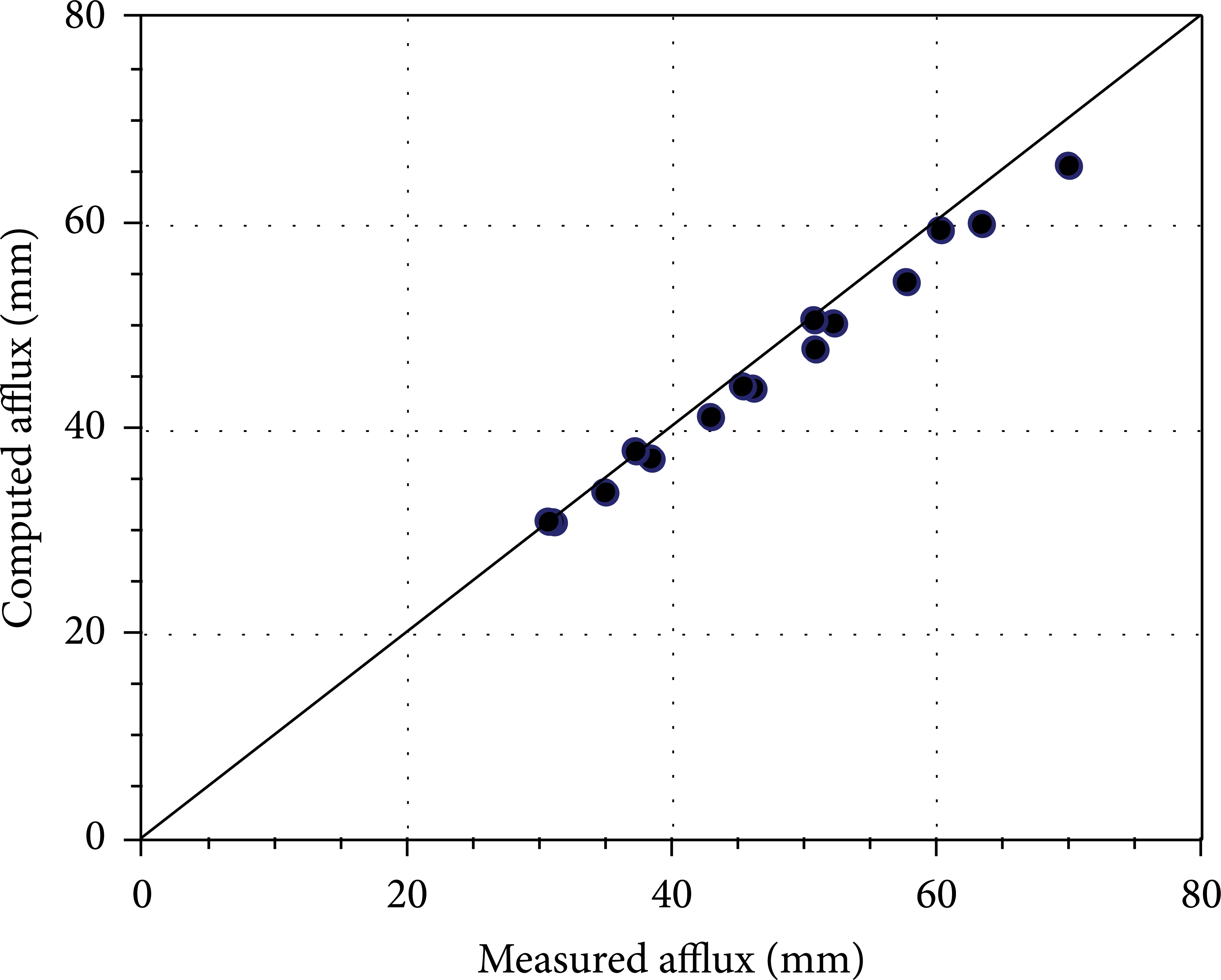
Comparison of computed and measured afflux values.

Figure 7:

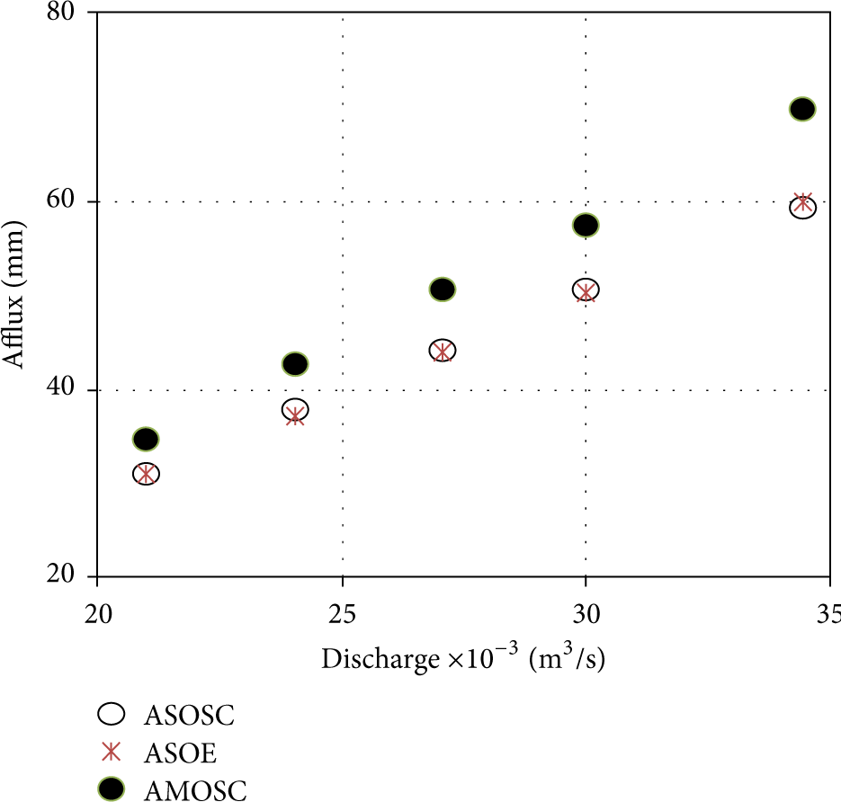
Comparison of computed afflux and discharge values for each bridge model.

5. Conclusions

The purpose of this study was to investigate the performance of a VOF based CFD software with respect to accurate prediction of the water surface profiles using the extensive experimental data that were collected through bridge constrictions with three different types of bridge openings in a compound channel. The k-ε turbulence closure model was used to determine turbulent viscosity.

The results showed that the performance and ability of commercially available CFD software, FLOW-3D, to model backwater profiles for various bridge geometries and flow rates in a two-stage channel generally appear great. The computed and measured water surface profiles downstream of bridges for all cases are in very good agreements. Therefore, CFD models can be recommended to use as a supplementary tool throughout the bridge design process.

Grid spacing in the use of 3D model played very important role in terms of both accuracy and simulation time. It was seen that there was a limit for selection of grid spacing particularly for places that were close to the solid surfaces, that is, bridges as well as places where flow characteristics changed rapidly, that is, immediately downstream of bridges. Use of larger grid in these places could result in unacceptable results. However, number of cells could safely be reduced by using finer grids only for places that are described above. Safely reducing the number of cells provides not only satisfactory results but also saving quite amount of simulation time, especially for the real case data.

In the present study, the findings are limited to the rigid boundary channel and low-flow conditions. Further analyses are needed to assess the performance of RANS based numerical models with different turbulence closures for similar flow conditions having loose boundary with a scour effect and high flow. In addition, due to the difference in friction coefficient between the main channel and the flood plain in nature, applications of a CFD model to field data will be very beneficial to evaluate its performance. Moreover, as a future study, the comparison among 1D, 2D, and 3D model results will provide a significant scientific contribution to the field.

Conflict of Interests

The author declares that there is no conflict of interests regarding the publication of this paper.

Footnotes

Acknowledgment

The author would like to thank Professor Dr. Galip Seckin and Professor Dr. Kutsi Savas Erduran for providing the experimental data and for sharing their valuable insights.

References

Shiono

and Knight

D. W.

, “Turbulent open-channel flows with variable depth across the channel,” Journal of Fluid Mechanics, vol. 222, pp. 617–646, 1991.

Biglari

and Sturm

T. W.

, “Numerical modeling of flow around bridge abutments in compound channel,” Journal of Hydraulic Engineering, vol. 124, no. 2, pp. 156–163, 1998.

Sumer

B. M.

, “Mathematical modelling of scour: a review,” Journal of Hydraulic Research, vol. 45, no. 6, pp. 723–735, 2007.

Melville

B. W.

, “Pier and abutment scour: Integrated approach,” Journal of Hydraulic Engineering, vol. 123, no. 2, pp. 125–136, 1997.

Kothyari

U. C.

and Ranga Raju

K. G.

, “Scour around spur dikes and bridge abutments,” Journal of Hydraulic Research, vol. 39, no. 4, pp. 367–374, 2001.

Ali

K. H. M.

and Karim

, “Simulation of flow around piers,” Journal of Hydraulic Research, vol. 40, no. 2, pp. 161–174, 2002.

Oliveto

and Hager

W. H.

, “Further results to time-dependent local scour at bridge elements,” Journal of Hydraulic Engineering, vol. 131, no. 2, pp. 97–105, 2005.

Dey

and Barbhuiya

A. K.

, “3D flow field in a scour hole at a wing-wall abutment,” Journal of Hydraulic Research, vol. 44, no. 1, pp. 33–50, 2006.

Johnson

P. A.

Sheeder

S. A.

, and Newlin

J. T.

, “Waterway transitions at US bridges,” Water and Environment Journal, vol. 24, no. 4, pp. 274–281, 2010.

10.

Graf

W. H.

and Istiarto

, “Flow pattern in the scour hole around a cylinder,” Journal of Hydraulic Research, vol. 40, no. 1, pp. 13–20, 2002.

11.

Haltigin

T. W.

Biron

P. M.

, and Lapointe

M. F.

, “Three-dimensional numerical simulation of flow around stream deflectors: the effect of obstruction angle and length,” Journal of Hydraulic Research, vol. 45, no. 2, pp. 227–238, 2007.

12.

Kaatz

K. J.

and James

W. P.

, “Analysis of alternatives for computing backwater at bridges,” Journal of Hydraulic Engineering, vol. 123, no. 9, pp. 784–792, 1997.

13.

Seckin

and Atabay

, “Experimental backwater analysis around bridge waterways,” Canadian Journal of Civil Engineering, vol. 32, no. 6, pp. 1015–1029, 2005.

14.

Crowder

R. A.

Pepper

A. T.

Whitlow

Sleigh

Wright

, and Tomlin

, “Benchmarking of hydraulic river modelling software packages,” Environment Agency Research Technical Report W5-105/TR0, 2004.

15.

Atabay

, “Accuracy of the ISIS bridge methods for prediction of afflux at high flows,” Water and Environment Journal, vol. 22, no. 1, pp. 64–73, 2008.

16.

Mantz

and Benn

, “Computation of afflux ratings and water surface profiles,” Proceedings of the Institution of Civil Engineers: Water Management, vol. 162, no. 1, pp. 41–55, 2009.

17.

Erduran

K. S.

Kutija

, and Hewett

C. J. M.

, “Performance of finite volume solutions to the shallow water equations with shock-capturing schemes,” International Journal for Numerical Methods in Fluids, vol. 40, no. 10, pp. 1237–1273, 2002.

18.

Liu

Zhou

J. G.

, and Burrows

, “Bridge afflux predictions using the Lattice Boltzmann method,” Procedia Environmental Sciences, vol. 2, pp. 1881–1893, 2010.

19.

Flow Science, Flow-3D User's Manuals, Flow Science, Santa Fe, NM, USA, 2007.

20.

Johnson

M. C.

and Savage

B. M.

, “Physical and numerical comparison of flow over ogee spillway in the presence of tailwater,” Journal of Hydraulic Engineering, vol. 132, no. 12, pp. 1353–1357, 2006.

21.

Kocaman

and Ozmen-Cagatay

, “The effect of lateral channel contraction on dam break flows: laboratory experiment,” Journal of Hydrology, vol. 432–433, pp. 145–153, 2012.

22.

Kocaman

Seckin

, and Erduran

K. S.

, “3D model for prediction of flow profiles around bridges,” Journal of Hydraulic Research, vol. 48, no. 4, pp. 521–525, 2010.

23.

Erduran

K. S.

Seckin

Kocaman

, and Atabay

, “3D numerical modelling of flow around skewed bridge crossing,” Engineering Applications of Computational Fluid Mechanics, vol. 6, no. 3, pp. 475–489, 2012.

24.

Atabay

and Knight

D. W.

, “Bridge afflux experiments in compound channels,” Technical Paper Presented for JBA Consulting Engineers & Scientists and the Environment Agency, University of Birmingham, Birmingham, UK, 2002.

25.

Seckin

Knight

D. W.

Atabay

, and Seckin

, “Bridge afflux experiments in compound channels,” Tech. Rep., JBA Consulting and the Environment Agency, University of Birmingham, Birmingham, UK, 2004.

26.

Seckin

Haktanir

, and Knight

D. W.

, “A simple method for estimating flood flow around bridges,” Proceedings of the Institution of Civil Engineers: Water Management, vol. 160, no. 4, pp. 195–202, 2007.

27.

JBA Consulting, “AEHR Hydraulic performance of river bridges and other structures at high flows, phase 2: afflux estimator hydraulic reference,” Environment Agency R&D Project: JBA Consulting, Skipton, W5A-065, 2006.

28.

JBA Consulting, “Defra/Environment Agency Afflux Estimation System (AES) User Guide,” Flood and Coastal Defence R&D Programme, JBA Consulting, Skipton, UK, 2007.

29.

Hirt

C. W.

and Sicilian

J. M.

, “A porosity technique for the definition of obstacles in rectangular cell meshes,” in Proceeding of the 4th International Conference on Ship Hydrodynamics, pp. 1–19, National Academy of Science, Washington, Wash, USA, 1985.

30.

Hirt

C. W.

, “Volume-fraction techniques: powerful tools for flow modeling,” Flow Science Report FSI-92-00-02, Flow Science, Santa Fe, NM, USA, 1992.

31.

Hirt

C. W.

and Nichols

B. D.

, “Volume of fluid (VOF) method for the dynamics of free boundaries,” Journal of Computational Physics, vol. 39, no. 1, pp. 201–225, 1981.

32.

Ozmen-Cagatay

and Kocaman

, “Dam-break flows during initial stage using SWE and RANS approaches,” Journal of Hydraulic Research, vol. 48, no. 5, pp. 603–611, 2010.

33.

Wilcox

D. C.

, Turbulence Modelling for CFD, DCW Industries, La Canada, Calif, USA, 2000.

34.

Launder

B. E.

and Spalding

D. B.

, “The numerical computation of turbulent flows,” Computer Methods in Applied Mechanics and Engineering, vol. 3, no. 2, pp. 269–289, 1974.

35.

Seckin

Yurtal

, and Haktanir

, “Contraction and expansion losses through bridge constrictions,” Journal of Hydraulic Engineering, vol. 124, no. 5, pp. 546–549, 1998.

36.

Hunt

Brunner

G. W.

, and Larock

B. E.

, “Flow transitions in bridge backwater analysis,” Journal of Hydraulic Engineering, vol. 125, no. 9, pp. 981–983, 1999.

37.

Picek

Havlik

Mattas

, and Mares

, “Hydraulic calculation of bridges at high water stages,” Journal of Hydraulic Research, vol. 45, no. 3, pp. 400–406, 2007.

38.

Martín-Vide

J. P.

and Prió

J. M.

, “Backwater of arch bridges under free and submerged conditions,” Journal of Hydraulic Research, vol. 43, no. 5, pp. 515–521, 2005.

Prediction of Backwater Profiles due to Bridges in a Compound Channel Using CFD

Abstract

1. Introduction

2. Experimental Work

3. Numerical Model

3.1. RANS Solution with k-ε Turbulence Model

3.2. Solution Domain, Boundary, and Initial Conditions

4. Results and Discussion

4.1. Computational Meshes

4.2. Backwater Profiles and Afflux Values

5. Conclusions

Conflict of Interests

Footnotes

Acknowledgment

References