Study on Accuracy of the High-Resolution Schemes

Abstract

The high-resolution (HR) schemes have been widely used as they can achieve the numerical solution without oscillation and artificial diffusion, especially for convection-dominated problems. However, there still have arguments about the order of accuracy of HR schemes, especially about the extreme value of the solution. In this paper, it is proved that any HR scheme designed in the NVD diagram has second-order accuracy when its combined segments totally locate in the BAIR region. In other words, it has been verified in our study that the segments, which have low-order accuracy when independently employed, have at least second-order accuracy when locate in BAIR region by analysis of two implementation methods of HR scheme and also a number of numerical examples. Meanwhile Richardson extrapolation has been used to estimate the order of accuracy of HR schemes which achieve the same conclusion.

1. Introduction

How to discretize the convective term in the governing equation, in order to acquire bounded and accurate numerical solution in the convection-dominated problems, has become one of the research keynotes in the field of computational fluid dynamics and numerical heat transfer. Some certain lower-order schemes, such as the first-order upwind (FUD) scheme, can present unconditionally stability in the numerical simulation procedure. However, when such lower-order schemes are used to discretize the convective term, numerical false diffusion would be caused, thus it can degrade the accuracy of the results, especially in the computational domain with sharp gradients, which means that these lower-order schemes cannot illustrate the physical problem perfectly due to the false diffusion. Therefore, some schemes, such as QUICK (Quadratic Upstream Interpolation for Convective Kinematics) scheme and CD (second-order central difference) scheme, are popular due to their higher-order accuracy. When these higher-order schemes are adopted, they can guarantee the order of accuracy of results, that means we can obtain more accurate numerical solution; but it would cause unphysical oscillation or overshoot/undershoot (unbounded solution) when grid Peclet number exceeds certain limit or a sharp change of profile exists in the computational domain, which lead to the low-accuracy of result, especially for the CD scheme which would result in obvious oscillation, overshoot/undershoot and instability.

Therefore, researchers in this field make attempts to develop the discrete scheme which can guarantee the boundedness and accuracy of the numerical solution. The high-resolution (HR) schemes proposed in recent years can overcome the above drawbacks which means HR schemes cannot only eliminate nonphysical oscillation and overshoot/undershoot, but also weaken the false diffusion and guarantee the stability of the solution procedure. Early, HR schemes are developed on the basis of total variation diminishing (TVD) proposed by Harten [1]; after that Gaskell and Lau proposed normalized variable formulation (NVF) and the convective boundedness criterion (CBC) [2], and then the definitions of HR schemes can be illustrated in normalized variable diagram (NVD) [3] after normalized. Some HR schemes developed in recent years, such as HOAB [4], HLPA [5], MINMOD [1], MUSCL [6], SMART [2] and STOIC [7], are found to obtain the results which are accurate with the absence of unphysical oscillation and artificial diffusion.

The research on the boundedness and accuracy of HR schemes has become a key point. It has been generally considered that the HR scheme has at least second-order accuracy on the whole when its characteristic line passes through node Q [8] in NVD (see Figure 2), that is when HR scheme is used in the physical problem without extreme value of solution, it has at least second-order accuracy. However, when there is the extreme point in the physical problem, researchers hold different views on the accuracy of HR schemes: Leonard indicated that the characteristic line which is near the extreme value of solution is of first-order accuracy, and the adoption of HR scheme at the extreme point would not degrade the order of accuracy of the overall algorithm [3]; Gaskell and Lau pointed out that the adoption of HR scheme at the extreme point of solution is a second-order approximation only through the adoption of the form containing QUICK scheme and correction term [2]; Sweby held the view that at the extreme point of the solution the second-order accuracy must be lost [9]; Wei et al. concluded that the scheme possesses at least second-order accuracy in any condition when its characteristic line locates within BAIR (Boundedness accuracy and interpolative reasonableness) region [4]. Thus it can be seen that the discussions about the order of accuracy of HR schemes, especially about that at the extreme point of solution, have not reached an agreement yet. In this paper the accuracy of HR schemes are discussed to investigate whether the HR schemes locating in the BAIR region, particularly at the extreme point, have at least second-order accuracy or not. The layout is as follows. In Section 2, the order of accuracy of HR schemes has been analyzed. And a number of numerical examples are shown in Section 3 to verify the analysis in Section 2. Finally, related conclusions are given in Section 4.

2. Analysis of the Accuracy of HR Schemes

2.1. Normalized Variable Formulation

The value of cell face is involved when a finite volume method is used to discretize the governing equation. Generally the value of cell face is acquired by the interpolation of the values of its nearby nodes. In a one-dimensional uniform grid system, the symbol U, C, and D are referred as the upstream, central and downstream node, respectively, and the symbol frepresents the cell face (see Figure 1). Then the interpolation of cell face values can be written as: ϕ _f = F(ϕ _U ,ϕ _C ,ϕ _D ). Introducing the following normalized variable:

${\tilde{\varphi }}_{}=\frac{\varphi -{\varphi }_U}{{\varphi }_D-{\varphi }_U}.$

(1)

Note that ${\tilde{\varphi }}_U=\mathrm{0}$ and ${\tilde{\varphi }}_D=\mathrm{1}$ , and the function of cell face value is only associated with ${\tilde{\varphi }}_C$ after normalized, that is: ${\tilde{\varphi }}_f=F({\tilde{\varphi }}_C)$ . The difference scheme can be defined by normalized variable, for example SUD scheme and CD scheme can be represented respectively as: $(1)\mathrm{\hspace{0.17em}\hspace{0.17em}}{\tilde{\varphi }}_f=\mathrm{1.5}{\tilde{\varphi }}_C$ for SUD scheme; $(2)\mathrm{\hspace{0.17em}\hspace{0.17em}}{\tilde{\varphi }}_f=\mathrm{0.5}+\mathrm{0.5}{\tilde{\varphi }}_C$ for CD scheme. The normalized expressions of several common used HR schemes (MINMOD [1], MUSCL [6], SMART [2], STOIC [7], HOAB [4] and HLPA [5]) are illustrated in Table 1.

Table 1:

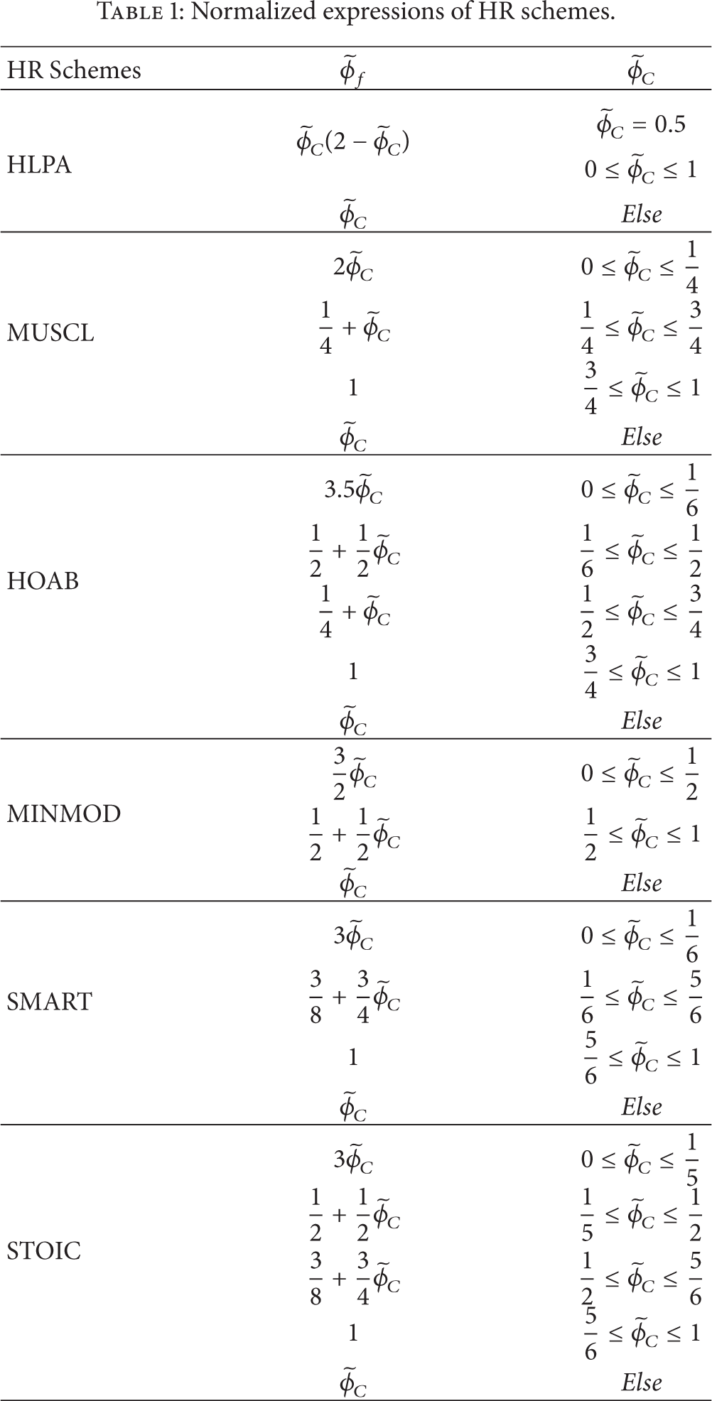
Normalized expressions of HR schemes.

HR Schemes	${\tilde{\mathrm{\varphi }}}_f$	${\tilde{\mathrm{\varphi }}}_C$
HLPA	${\tilde{\mathrm{\varphi }}}_C(\mathrm{2}-{\tilde{\mathrm{\varphi }}}_C)$	${\tilde{\varphi }}_C=\mathrm{0.5}$
		$\mathrm{0}\le {\tilde{\mathrm{\varphi }}}_C\le \mathrm{1}$
	${\tilde{\mathrm{\varphi }}}_C$	Else
MUSCL	$\mathrm{2}{\tilde{\mathrm{\varphi }}}_C$	$\mathrm{0}\le {\tilde{\mathrm{\varphi }}}_C\le \frac{\mathrm{1}}{\mathrm{4}}$
	$\frac{\mathrm{1}}{\mathrm{4}}+{\tilde{\mathrm{\varphi }}}_C$	$\frac{\mathrm{1}}{\mathrm{4}}\le {\tilde{\mathrm{\varphi }}}_C\le \frac{\mathrm{3}}{\mathrm{4}}$
	1	$\frac{\mathrm{3}}{\mathrm{4}}\le {\tilde{\mathrm{\varphi }}}_C\le \mathrm{1}$
	${\tilde{\mathrm{\varphi }}}_C$	Else
HOAB	$\mathrm{3.5}{\tilde{\mathrm{\varphi }}}_C$	$\mathrm{0}\le {\tilde{\mathrm{\varphi }}}_C\le \frac{\mathrm{1}}{\mathrm{6}}$
	$\frac{\mathrm{1}}{\mathrm{2}}+\frac{\mathrm{1}}{\mathrm{2}}{\tilde{\mathrm{\varphi }}}_C$	$\frac{\mathrm{1}}{\mathrm{6}}\le {\tilde{\mathrm{\varphi }}}_C\le \frac{\mathrm{1}}{\mathrm{2}}$
	$\frac{\mathrm{1}}{\mathrm{4}}+{\tilde{\mathrm{\varphi }}}_C$	$\frac{\mathrm{1}}{\mathrm{2}}\le {\tilde{\mathrm{\varphi }}}_C\le \frac{\mathrm{3}}{\mathrm{4}}$
	1	$\frac{\mathrm{3}}{\mathrm{4}}\le {\tilde{\mathrm{\varphi }}}_C\le \mathrm{1}$
	${\tilde{\mathrm{\varphi }}}_C$	Else
MINMOD	$\frac{\mathrm{3}}{\mathrm{2}}{\tilde{\mathrm{\varphi }}}_C$	$\mathrm{0}\le {\tilde{\mathrm{\varphi }}}_C\le \frac{\mathrm{1}}{\mathrm{2}}$
	$\frac{\mathrm{1}}{\mathrm{2}}+\frac{\mathrm{1}}{\mathrm{2}}{\tilde{\mathrm{\varphi }}}_C$	$\frac{\mathrm{1}}{\mathrm{2}}\le {\tilde{\mathrm{\varphi }}}_C\le \mathrm{1}$
	${\tilde{\mathrm{\varphi }}}_C$	Else
SMART	$\mathrm{3}{\tilde{\mathrm{\varphi }}}_C$	$\mathrm{0}\le {\tilde{\mathrm{\varphi }}}_C\le \frac{\mathrm{1}}{\mathrm{6}}$
	$\frac{\mathrm{3}}{\mathrm{8}}+\frac{\mathrm{3}}{\mathrm{4}}{\tilde{\mathrm{\varphi }}}_C$	$\frac{\mathrm{1}}{\mathrm{6}}\le {\tilde{\mathrm{\varphi }}}_C\le \frac{\mathrm{5}}{\mathrm{6}}$
	1	$\frac{\mathrm{5}}{\mathrm{6}}\le {\tilde{\mathrm{\varphi }}}_C\le \mathrm{1}$
	${\tilde{\mathrm{\varphi }}}_C$	Else
STOIC	$\mathrm{3}{\tilde{\mathrm{\varphi }}}_C$	$\mathrm{0}\le {\tilde{\mathrm{\varphi }}}_C\le \frac{\mathrm{1}}{\mathrm{5}}$
	$\frac{\mathrm{1}}{\mathrm{2}}+\frac{\mathrm{1}}{\mathrm{2}}{\tilde{\mathrm{\varphi }}}_C$	$\frac{\mathrm{1}}{\mathrm{5}}\le {\tilde{\mathrm{\varphi }}}_C\le \frac{\mathrm{1}}{\mathrm{2}}$
	$\frac{\mathrm{3}}{\mathrm{8}}+\frac{\mathrm{3}}{\mathrm{4}}{\tilde{\mathrm{\varphi }}}_C$	$\frac{\mathrm{1}}{\mathrm{2}}\le {\tilde{\mathrm{\varphi }}}_C\le \frac{\mathrm{5}}{\mathrm{6}}$
	1	$\frac{\mathrm{5}}{\mathrm{6}}\le {\tilde{\mathrm{\varphi }}}_C\le \mathrm{1}$
	${\tilde{\mathrm{\varphi }}}_C$	Else

Figure 1:

Uniform grid system.

Figure 2:

NVD of SUD scheme and CD scheme.

Taking ${\tilde{\varphi }}_C$ as an independent variable and ${\tilde{\varphi }}_f$ as a dependent variable, the normalized scheme can be expressed in the form of characteristic line, and the diagram that can illustrate the relationship between ${\tilde{\varphi }}_C$ and ${\tilde{\varphi }}_f$ is called normalized variable diagram (NVD). The definitions of SUD scheme and CD scheme in the NVD are shown in Figure 2. Here for brevity, the region where ${\tilde{\varphi }}_C\in [\mathrm{0,1}]$ in NVD is named as inner domain, and ${\tilde{\varphi }}_C\notin [\mathrm{0,1}]$ as outer domain, and according to CBC, the HR schemes are all presented in the form of FUD scheme in the outer domain of the NVD, that is ${\tilde{\varphi }}_f={\tilde{\varphi }}_C$ .

2.2. BAIR Condition

As SUD and CD schemes, the HR schemes can be represented by normalized variable as well, which means that the definition of HR schemes can be illustrated in NVD. The BAIR condition proposed by Wei et al. [4] refers to the region in NVD that satisfies the following conditions:

1. CBC proposed by Gaskell and Lau [2].

2. The line of a scheme passing through O(0, 0), Q(0.5, 0.75), and P(1, 1) in the NVD.

3. Interpolative reasonableness.

Thus the region that satisfies the BAIR condition is the shaded area shown in Figure 3. From Figure 3, it can be seen that the HR composite schemes satisfying BAIR condition own the following properties: (1) the line of a scheme is located between the lines of SUD scheme and CD scheme in the inner domain; (2) the line happens to coincide with that of FUD scheme in the outer domain; (3) any HR scheme would pass through node O, Q, and P mentioned above. The characteristic lines of several common-used HR schemes, such as MINMOD [1], HLPA, and SMART, all fall into the BAIR region.

Figure 3:

The region of BAIR.

2.3. Interpolation Method

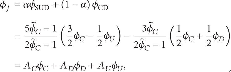
As mentioned above, cell face value can be obtained by the interpolation of adjacent node values via various difference schemes. From the first two properties of HR schemes satisfying BAIR condition, it is known that any difference scheme falling into this region can be written as a combination of SUD scheme and CD scheme (as SCSD scheme proposed in reference [10], here we name it the rewritten scheme for short), then the cell face value is:

${\varphi }_f=\alpha {\varphi }_{\text{SUD}}+\left(\mathrm{1}-\alpha \right){\varphi }_{\text{CD}}.$

(2)

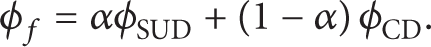
Considering that ϕ_SUD = 1.5ϕ _C − 0.5ϕ _U , ϕ_CD = 0.5ϕ _C + 0.5ϕ _D , (2) can be normalized as:

${\tilde{\varphi }}_f=\alpha {\tilde{\varphi }}_{\text{SUD}}+\left(\mathrm{1}-\alpha \right){\tilde{\varphi }}_{\text{CD}}.$

(3)

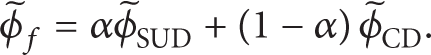
The first and the second term on the right side of (3) represent the normalized SUD scheme and CD scheme respectively, in which ${\tilde{\varphi }}_{\text{SUD}}=\mathrm{1.5}{\tilde{\varphi }}_C$ and ${\tilde{\varphi }}_{\text{CD}}=\mathrm{0.5}+\mathrm{0.5}{\tilde{\varphi }}_C$ . The value of coefficient α represents the proportion of SUD scheme which depends on the type of scheme. When α = 1.0 it means that SUD scheme is employed for the cell-face value interpolation, and α = 0.0 means CD scheme is employed.

For schemes satisfying the BAIR condition, the characteristic lines lie between the lines of SUD scheme and CD scheme, which means the value of ${\tilde{\varphi }}_f$ is between the values of the above two schemes with the same ${\tilde{\varphi }}_C$ . Thus it can obtain α ∈ [0, 1], which can guarantee at least second-order accuracy of the rewritten HR schemes. In addition, the truncation error term of the SUD scheme according to the Taylor series expansion is − (3/4)Δx²(∂²ϕ/∂x²), and that of CD scheme is (1/4)Δx²(∂²ϕ/∂x²), thus that of the rewritten scheme is:

$\begin{array}{c}o\left(\mathrm{\Delta }{x}^{\mathrm{2}}\right)=\left[-\alpha \frac{\mathrm{3}}{\mathrm{4}}+\left(\mathrm{1}-\alpha \right)\frac{\mathrm{1}}{\mathrm{4}}\right]\mathrm{\Delta }{x}^{\mathrm{2}}\frac{{\partial }^{\mathrm{2}}\varphi }{\partial x^{\mathrm{2}}}\\ =\left(\frac{\mathrm{1}}{\mathrm{4}}-\alpha \right)\mathrm{\Delta }{x}^{\mathrm{2}}\frac{{\partial }^{\mathrm{2}}\varphi }{\partial x^{\mathrm{2}}}.\end{array}$

(4)

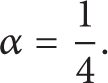
On the basis of value range of α and the above truncation error term shown in (4), the value range of truncation error of the rewritten scheme is [− 0.75Δx²,0.25Δx²], indicating that the rewritten scheme is at least second-order accurate, while it is third-order accurate particularly when α = 0.25.

2.3.1. Derivation of α

For brevity, QUICK scheme is taken as an example here to present interpolation using (2), in order to explain the process of getting α value. The original form of QUICK scheme is:

${\varphi }_f=\frac{\mathrm{1}}{\mathrm{8}}\left(\mathrm{3}{\varphi }_D+\mathrm{6}{\varphi }_C-{\varphi }_U\right).$

(5)

Substitute (5) into (2), we have

$\alpha =\frac{\mathrm{1}}{\mathrm{4}}.$

(6)

Then, the rewritten form of QUICK scheme is obtained,

${\varphi }_f=\frac{\mathrm{1}}{\mathrm{4}}{\varphi }_{\text{SUD}}+\frac{\mathrm{3}}{\mathrm{4}}{\varphi }_{\text{CD}}.$

(7)

Equation (7) is also the expression of cell face value when the QUICK scheme is used to discretize governing equation.

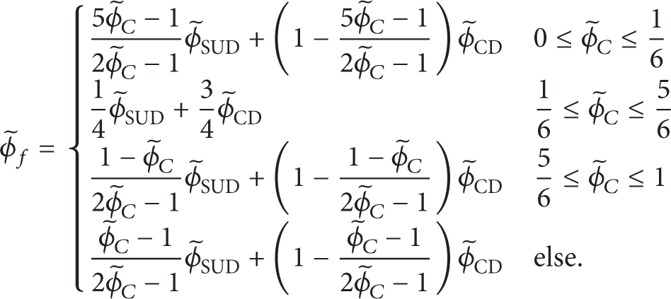
HR schemes usually consist of several difference schemes, and any difference scheme satisfying BAIR condition can be rewritten in the form like (2), that is to say they can be written in a form combining with α, SUD scheme and CD scheme together. Here in order to explain the process of derivation of α for HR schemes, we take SMART as example, which is:

${\tilde{\varphi }}_f=\{\begin{array}{cc}\mathrm{3}{\tilde{\varphi }}_C\hfill & \mathrm{0}\le {\tilde{\varphi }}_C\le \frac{1}{6}\hfill \\ \frac{\mathrm{3}}{\mathrm{8}}+\frac{\mathrm{3}}{\mathrm{4}}{\tilde{\varphi }}_C\hfill & \frac{\mathrm{1}}{\mathrm{6}}\le {\tilde{\varphi }}_C\le \frac{\mathrm{5}}{\mathrm{6}}\hfill \\ \mathrm{1}\hfill & \frac{\mathrm{5}}{\mathrm{6}}\le {\tilde{\varphi }}_C\le \mathrm{1}\hfill \\ {\tilde{\varphi }}_C\hfill & \text{else}.\hfill \end{array}$

(8)

It can be seen that SMART is composed of four difference schemes, among which every scheme can be expressed in the form shown in (3), and different intervals of ${\tilde{\varphi }}_C$ have a corresponding α, respectively. Here one of the SMART segments is taken as an example to derive the α, when $\mathrm{0}<{\tilde{\varphi }}_C\le \mathrm{1}/\mathrm{6}$ we have:

$\mathrm{3}{\tilde{\varphi }}_C=\alpha {\tilde{\varphi }}_{\text{SUD}}+\left(\mathrm{1}-\alpha \right){\tilde{\varphi }}_{\text{CD}},$

(9)

where ${\tilde{\varphi }}_{\text{SUD}}=\mathrm{1.5}{\tilde{\varphi }}_C$ and ${\tilde{\varphi }}_{\text{CD}}=\mathrm{0.5}+\mathrm{0.5}{\tilde{\varphi }}_C$ . After simplifying (9) we get:

$\alpha =\frac{\mathrm{5}{\tilde{\varphi }}_C-\mathrm{1}}{\mathrm{2}{\tilde{\varphi }}_C-\mathrm{1}}.$

(10)

Then the other segments of SMART can be obtained in the same way, from which the SMRAT scheme can be rewritten as:

${\tilde{\varphi }}_f=\{\begin{array}{cc}\frac{\mathrm{5}{\tilde{\varphi }}_C-\mathrm{1}}{\mathrm{2}{\tilde{\varphi }}_C-\mathrm{1}}{\tilde{\varphi }}_{\text{SUD}}+\left(\mathrm{1}-\frac{\mathrm{5}{\tilde{\varphi }}_C-\mathrm{1}}{\mathrm{2}{\tilde{\varphi }}_C-\mathrm{1}}\right){\tilde{\varphi }}_{\text{CD}}\hfill & \mathrm{0}\le {\tilde{\varphi }}_C\le \frac{\mathrm{1}}{\mathrm{6}}\hfill \\ \frac{\mathrm{1}}{\mathrm{4}}{\tilde{\varphi }}_{\text{SUD}}+\frac{\mathrm{3}}{\mathrm{4}}{\tilde{\varphi }}_{\text{CD}}\hfill & \frac{\mathrm{1}}{\mathrm{6}}\le {\tilde{\varphi }}_C\le \frac{\mathrm{5}}{\mathrm{6}}\hfill \\ \frac{\mathrm{1}-{\tilde{\varphi }}_C}{\mathrm{2}{\tilde{\varphi }}_C-\mathrm{1}}{\tilde{\varphi }}_{\text{SUD}}+\left(\mathrm{1}-\frac{\mathrm{1}-{\tilde{\varphi }}_C}{\mathrm{2}{\tilde{\varphi }}_C-\mathrm{1}}\right){\tilde{\varphi }}_{\text{CD}}\hfill & \frac{\mathrm{5}}{\mathrm{6}}\le {\tilde{\varphi }}_C\le \mathrm{1}\hfill \\ \frac{{\tilde{\varphi }}_C-\mathrm{1}}{\mathrm{2}{\tilde{\varphi }}_C-\mathrm{1}}{\tilde{\varphi }}_{\text{SUD}}+\left(\mathrm{1}-\frac{{\tilde{\varphi }}_C-\mathrm{1}}{\mathrm{2}{\tilde{\varphi }}_C-\mathrm{1}}\right){\tilde{\varphi }}_{\text{CD}}\hfill & \text{else}.\hfill \end{array}$

(11)

2.3.2. Values of α for Different HR Schemes

Through above analysis, it is found that HR schemes lying in the BAIR region can be described by expressions containing coefficient α. The values of α in different intervals of several common used HR schemes (MINMOD [1], MUSCL [6], SMART [2], STOIC [7], HOAB [4] and HLPA [5]) are illustrated in Table 2.

Table 2:

Value of α.

HR Schemes	α	${\tilde{\mathrm{\varphi }}}_C$
HLPA	0.5	${\tilde{\varphi }}_C=\mathrm{0.5}$
	$\frac{{\tilde{\mathrm{\varphi }}}_C(\mathrm{3}-\mathrm{2}{\tilde{\mathrm{\varphi }}}_C)-\mathrm{1}}{\mathrm{2}{\tilde{\mathrm{\varphi }}}_C-\mathrm{1}}$	$\mathrm{0}\le {\tilde{\mathrm{\varphi }}}_C\le \mathrm{1}$
	$\frac{{\tilde{\mathrm{\varphi }}}_C-\mathrm{1}}{\mathrm{2}{\tilde{\mathrm{\varphi }}}_C-\mathrm{1}}$	Else
MUSCL	$\frac{\mathrm{3}{\tilde{\mathrm{\varphi }}}_C-\mathrm{1}}{\mathrm{2}{\tilde{\mathrm{\varphi }}}_C-\mathrm{1}}$	$\mathrm{0}\le {\tilde{\mathrm{\varphi }}}_C\le \frac{\mathrm{1}}{\mathrm{4}}$
	$\frac{\mathrm{1}}{\mathrm{2}}$	$\frac{\mathrm{1}}{\mathrm{4}}\le {\tilde{\mathrm{\varphi }}}_C\le \frac{\mathrm{3}}{\mathrm{4}}$
	$\frac{\mathrm{1}-{\tilde{\mathrm{\varphi }}}_C}{\mathrm{2}{\tilde{\mathrm{\varphi }}}_C-\mathrm{1}}$	$\frac{\mathrm{3}}{\mathrm{4}}\le {\tilde{\mathrm{\varphi }}}_C\le \mathrm{1}$
	$\frac{{\tilde{\mathrm{\varphi }}}_C-\mathrm{1}}{\mathrm{2}{\tilde{\mathrm{\varphi }}}_C-\mathrm{1}}$	Else
HOAB	$\frac{\mathrm{6}{\tilde{\mathrm{\varphi }}}_C-\mathrm{1}}{\mathrm{2}{\tilde{\mathrm{\varphi }}}_C-\mathrm{1}}$	$\mathrm{0}\le {\tilde{\mathrm{\varphi }}}_C\le \frac{\mathrm{1}}{\mathrm{6}}$
	0.0	$\frac{\mathrm{1}}{\mathrm{6}}\le {\tilde{\mathrm{\varphi }}}_C\le \frac{\mathrm{1}}{\mathrm{2}}$
	$\frac{\mathrm{1}}{\mathrm{2}}$	$\frac{\mathrm{1}}{\mathrm{2}}\le {\tilde{\mathrm{\varphi }}}_C\le \frac{\mathrm{3}}{\mathrm{4}}$
	$\frac{\mathrm{1}-{\tilde{\mathrm{\varphi }}}_C}{\mathrm{2}{\tilde{\mathrm{\varphi }}}_C-\mathrm{1}}$	$\frac{\mathrm{3}}{\mathrm{4}}\le {\tilde{\mathrm{\varphi }}}_C\le \mathrm{1}$
	$\frac{{\tilde{\mathrm{\varphi }}}_C-\mathrm{1}}{\mathrm{2}{\tilde{\mathrm{\varphi }}}_C-\mathrm{1}}$	Else
MINMOD	1.0	$\mathrm{0}\le {\tilde{\mathrm{\varphi }}}_C\le \frac{\mathrm{1}}{\mathrm{2}}$
	0.0	$\frac{\mathrm{1}}{\mathrm{2}}\le {\tilde{\mathrm{\varphi }}}_C\le \mathrm{1}$
	$\frac{{\tilde{\mathrm{\varphi }}}_C-\mathrm{1}}{\mathrm{2}{\tilde{\mathrm{\varphi }}}_C-\mathrm{1}}$	Else
SMART	$\frac{\mathrm{5}{\tilde{\mathrm{\varphi }}}_C-\mathrm{1}}{\mathrm{2}{\tilde{\mathrm{\varphi }}}_C-\mathrm{1}}$	$\mathrm{0}\le {\tilde{\mathrm{\varphi }}}_C\le \frac{\mathrm{1}}{\mathrm{6}}$
	$\frac{\mathrm{1}}{\mathrm{4}}$	$\frac{\mathrm{1}}{\mathrm{6}}\le {\tilde{\mathrm{\varphi }}}_C\le \frac{\mathrm{5}}{\mathrm{6}}$
	$\frac{\mathrm{1}-{\tilde{\mathrm{\varphi }}}_C}{\mathrm{2}{\tilde{\mathrm{\varphi }}}_C-\mathrm{1}}$	$\frac{\mathrm{5}}{\mathrm{6}}\le {\tilde{\mathrm{\varphi }}}_C\le \mathrm{1}$
	$\frac{{\tilde{\mathrm{\varphi }}}_C-\mathrm{1}}{\mathrm{2}{\tilde{\mathrm{\varphi }}}_C-\mathrm{1}}$	Else
STOIC	$\frac{\mathrm{5}{\tilde{\mathrm{\varphi }}}_C-\mathrm{1}}{\mathrm{2}{\tilde{\mathrm{\varphi }}}_C-\mathrm{1}}$	$\mathrm{0}\le {\tilde{\mathrm{\varphi }}}_C\le \frac{\mathrm{1}}{\mathrm{5}}$
	0.0	$\frac{\mathrm{1}}{\mathrm{5}}\le {\tilde{\mathrm{\varphi }}}_C\le \frac{\mathrm{1}}{\mathrm{2}}$
	$\frac{\mathrm{1}}{\mathrm{4}}$	$\frac{\mathrm{1}}{\mathrm{2}}\le {\tilde{\mathrm{\varphi }}}_C\le \frac{\mathrm{5}}{\mathrm{6}}$
	$\frac{\mathrm{1}-{\tilde{\mathrm{\varphi }}}_C}{\mathrm{2}{\tilde{\mathrm{\varphi }}}_C-\mathrm{1}}$	$\frac{\mathrm{5}}{\mathrm{6}}\le {\tilde{\mathrm{\varphi }}}_C\le \mathrm{1}$
	$\frac{{\tilde{\mathrm{\varphi }}}_C-\mathrm{1}}{\mathrm{2}{\tilde{\mathrm{\varphi }}}_C-\mathrm{1}}$	Else

In order to express the value of α clearly, the relationship between α and ${\tilde{\varphi }}_C$ in the inner domain of the HR schemes shown in Table 2 is presented in Figure 4. α of different schemes in the outer domain can be presented in an identical way, and from $\alpha =({\tilde{\varphi }}_C-\mathrm{1})/(\mathrm{2}{\tilde{\varphi }}_C-\mathrm{1})$ we know that when ${\tilde{\varphi }}_C\to +\infty$ or ${\tilde{\varphi }}_C\to -\infty$ we have α → 0.5, which means when ${\tilde{\varphi }}_C\in (\mathrm{1},+\infty )$ we have α ∈ [0, 0.5) and when ${\tilde{\varphi }}_C\in (-\infty ,\mathrm{0})$ we get α ∈ (0.5, 1] (see Figure 5). Therefore it can be verified again that α ∈ [0, 1], and HR schemes have at least a second-order accuracy after rewritten.

Figure 4:

The value of α for different HR schemes.

Figure 5:

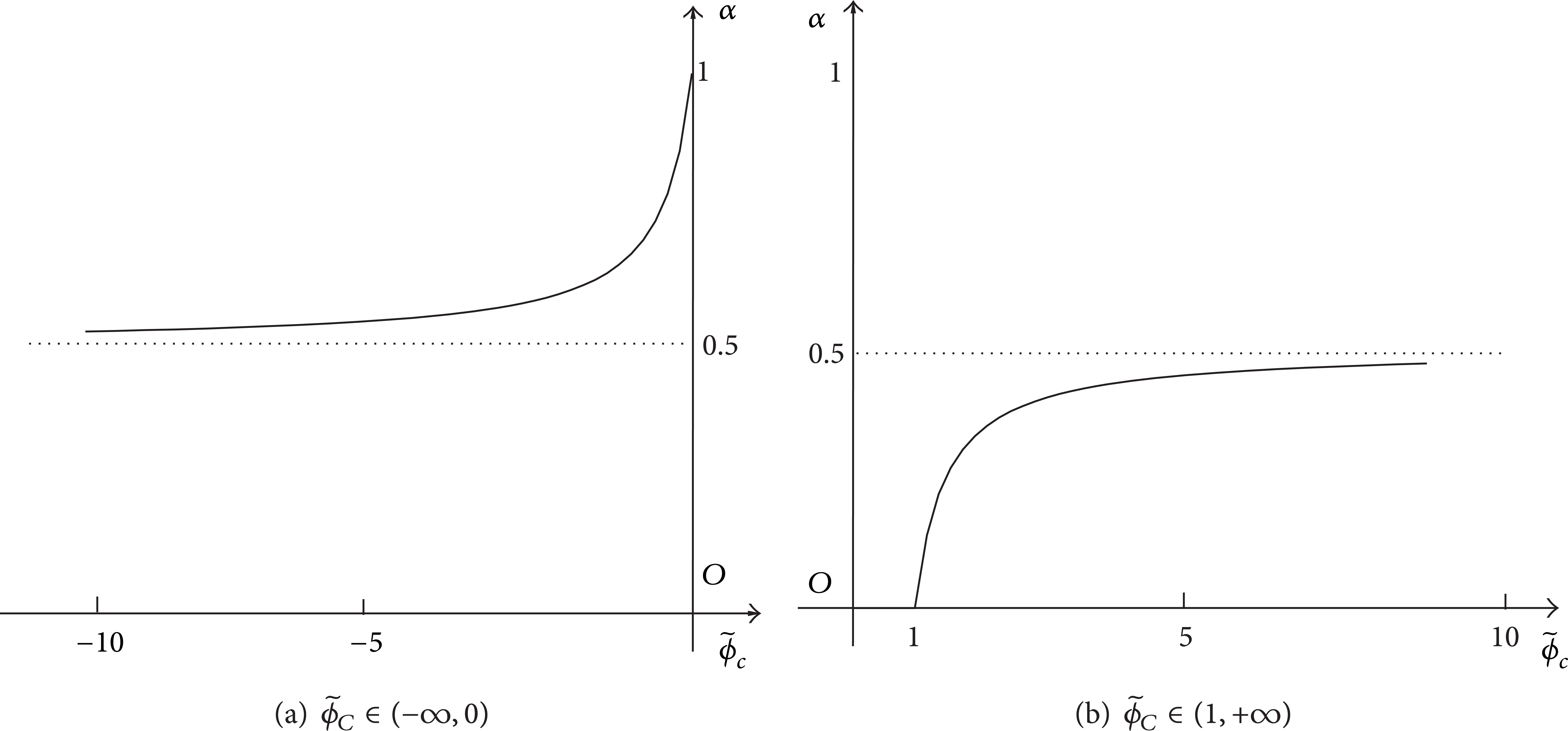
The value of α in the outer domain.

2.4. The Implementation of HR Schemes

The implementation of HR schemes is achieved through discretizing the governing equation using HR schemes. The difference between the implementations of HR schemes lies in the way to interpolate cell face value. There are two kinds of implementation methods of rewritten HR schemes (here the interval $\mathrm{0}\le {\tilde{\varphi }}_C\le \mathrm{1}/\mathrm{6}$ of SMART is taken as an example):

(1) Direct Implementation Method. In direct implementation method, HR schemes are employed in the interpolation directly. As α of rewritten SMART in the above interval is $\alpha =(\mathrm{5}{\tilde{\varphi }}_C-\mathrm{1})/(\mathrm{2}{\tilde{\varphi }}_C-\mathrm{1})$ , the interpolation of cell face value can be presented as:

$\begin{array}{l}{\varphi }_f=\alpha {\varphi }_{\text{SUD}}+\left(1-\alpha \right){\varphi }_{\text{CD}}\\ =\frac{5{\tilde{\varphi }}_C-1}{2{\tilde{\varphi }}_C-1}\left(\frac{3}{2}{\varphi }_C-\frac{1}{2}{\varphi }_U\right)-\frac{3{\tilde{\varphi }}_C}{2{\tilde{\varphi }}_C-1}\left(\frac{1}{2}{\varphi }_C+\frac{1}{2}{\varphi }_D\right)\\ =A_C{\varphi }_C+A_D{\varphi }_D+A_U{\varphi }_U,\end{array}$

(12)

where $A_C=\mathrm{3}(\mathrm{4}{\tilde{\varphi }}_C-\mathrm{1})/[\mathrm{2}(\mathrm{2}{\tilde{\varphi }}_C-\mathrm{1})]$ , $A_D=-\mathrm{3}{\tilde{\varphi }}_C/[\mathrm{2}(\mathrm{2}{\tilde{\varphi }}_C-\mathrm{1})]$ and $A_U=(\mathrm{1}-\mathrm{5}{\tilde{\varphi }}_C)/[\mathrm{2}(\mathrm{2}{\tilde{\varphi }}_C-\mathrm{1})]$ . And the solution mentioned in reference [2] is employed, that is the SUR (successive under-relaxation) iterative method, in which A _C , A _D and A _U containing α are regarded as the coefficients of discretized equation. Thus, it is equivalent to use the scheme that possesses at least second-order accuracy in the discrezition of convective term.

(2) Deferred Correction (DC) Method. In DC method, HR schemes have been introduced into the source term of discretized equation in the form of correction term, that is to say, DC method is adopted to discretize the convective term. Then the interpolation of cell face value can be presented as:

${\varphi }_f={\varphi }_C^{\text{new}}+{\left[\alpha {\varphi }_{\text{SUD}}+\left(1-\alpha \right){\varphi }_{\text{CD}}-{\varphi }_C\right]}^{\text{old}},$

(13)

where superscripts new and old represent numerical results of the present and last iteration layer, respectively, and the second term on the right side of (13) is the correction term which can be put into the source term of discretized equation. Since the first term on the right side of (13) is independent of the second term, the form of (13) is equivalent to use FUD scheme to discretize convective term. Substitute $\alpha =(\mathrm{5}{\tilde{\varphi }}_C-\mathrm{1})/(\mathrm{2}{\tilde{\varphi }}_C-\mathrm{1})$ into (13), we get:

${\varphi }_f={\varphi }_C^{\text{new}}+{\left[\left(3{\varphi }_C-2{\varphi }_U\right)-{\varphi }_C\right]}^{\text{old}}.$

(14)

If DC method is introduced into the original HR scheme, the expression of interpolation is:

${\varphi }_f={\varphi }_C^{\text{new}}+{\left[F\left({\tilde{\varphi }}_C\right)·\left({\varphi }_D-{\varphi }_U\right)+{\varphi }_U-{\varphi }_C\right]}^{\text{old}}.$

(15)

As is known, in this interval the original SMART is ${\tilde{\varphi }}_f=\mathrm{3}{\tilde{\varphi }}_C$ , and when introducing it to (15) the form of interpolation same with (13) can be obtained. It indicates that when DC method has been introduced into the discretization of convective term, the same expression of convective term can be gained in the discretized equation by the rewritten and the original HR schemes respectively, which means the rewritten and original HR schemes are of equivalence. However, considering the superiority of the latter in computation efficiency, the expression in (15) is employed when DC method is introduced. In addition, the introduction of DC method can improve the stability of solution only, and has no influence on the accuracy. Thus when the above two implementation methods of HR schemes are employed respectively and the solution reaches final convergence, the same results can be obtained, that is they are equivalent. Using the first implementation method, every segment of composite schemes, especially the FUD scheme segment in the outer domain, is replaced by schemes that possess second-order accuracy as α ∈ [0, 1]. On the other hand, employing the second implementation method, the interpolation of cell face value is ϕ _f = ϕ _C ^new in the outer domain, and it has been verified that the two kinds of implementation methods are equivalent and the segment of FUD scheme is replaced by second-order accurate schemes, that means the segment of FUD scheme is of second-order accuracy, so is the inner domain. Therefore, the employment of (15) has second-order accuracy, in other words, every segment of HR schemes that satisfies the BAIR condition is of at least second-order accuracy, though it may be indicated by Taylor series expansion that some segments of HR scheme, such as ${\tilde{\varphi }}_f=\mathrm{3}{\tilde{\varphi }}_C$ , have low-order accuracy when independently employed. The above statements are proved in Section 3 by a number of numerical examples.

3. Test Examples

In this section, the accuracy of HR scheme is explained in detail. First, the above two implementation methods of HR schemes are employed in the following test examples to verify the accuracy of HR schemes: (1) a pure convection problem of a stepwise profile in an oblique uniform velocity field (it is called 2D pure convection problem for short); (2) lid-driven flow in a square cavity with the given temperature boundary condition (it is called lid-driven flow in a square cavity for short). Second, by applying the Richardson extrapolation [11] in the second problem, the order of accuracy of HR schemes has been given. The following HR schemes have been adopted in both two problems: HOAB, HLPA, MINMOD, MUSCL, SMART and STOIC. The sum of the residual of discretized equation is:

$\text{RES}=\sum \left|a_P{\varphi }_P-\left(\sum _{\text{NB}=E,W,N,S}{a}_{\text{NB}}{\varphi }_{\text{NB}}+b\right)\right|,$

(16)

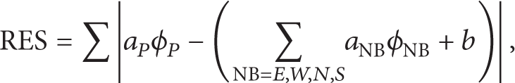
which can be referred as the convergence criterion, thus the convergence will be reached when the sum of the residual error is smaller than the set value (depending on specific problem).

3.1. Explanations of Test Examples

3.1.1. Problem 1: 2D Pure Convection Problem

This problem is shown in Figure 6. In an oblique uniform velocity field, the configuration of transportation scalar is a stepwise profile; the flow angle is 30°; the boundary condition of transportation scalar is also presented in Figure 6. A uniform grid system with 22 × 22 grids is used, and the convergence criterion is: RES < 10⁻⁵. In Figure 7, the scalar profiles at the mid-horizontal plane (y = 0.5) predicted by HLPA, MINMOD and SMART (representative and typical of the six HR schemes) are presented for comparison. Here, Solution I and Solution II represent the numerical solution of the first (see (12)) and the second (see (15)) implementation method, respectively. Figure 7 indicates that the results of two implementation methods agree well with each other. To analyze the results of the above two implementation methods quantitatively, the definitions of average deviation and the maximum deviation are given at first, which are:

$\begin{array}{c}\overline{\mathrm{err}}=\frac{{\sum }_{\text{all}\mathrm{\hspace{0.17em}\hspace{0.17em}}\text{nodes}}\left|{\varphi }_{\text{DC}}-{\varphi }_{C-S}\right|}{N^{\mathrm{2}}},\\ \text{er}{\text{r}}_{\max }=\max \left(\left|{\varphi }_{\text{DC}}-{\varphi }_{C-S}\right|\right),\end{array}$

(17)

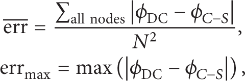
where ϕ_DC represents the results obtained by DC method shown in (15); ϕ_{C − S} represents the result obtained by the employment of rewritten scheme shown in (12), that is the original HR schemes have been replaced by the combination of two schemes of second-order accuracy, then the discretized equation contains α which represents the proportion of SUD scheme, and the coefficient matrix is a nine-diagonal matrix, and SUR iterative method has been used in solution; $\overline{\mathrm{err}}$ refers to average deviation and err_max refers to maximum deviation; N stands for the number of grid nodes. The derivation of the above two implementation methods of different HR schemes (still taking HLPA, MINMOD and SMRAT as examples) is presented in Table 3. When the computation reached the final convergence, the lines that are carried out by the two implementation methods of the same HR scheme are totally same in the same location of the computational domain, and every segment of composite schemes has been carried out by the two implementation methods during the solution. Moreover, the deviation in Table 3 shows that the difference between two implementation methods are less than 5 × 10⁻⁵, which can be convincingly explained that such differences are caused by round-off error. Then the equivalence of two implementation methods can be verified by the same results they acquired.

Table 3:

Deviation of two implementation methods for Problem 1.

	Deviation	HLPA	MINMOD	SMART
Θ	$\overline{\mathrm{err}}$	8.27 × 10−7	8.71 × 10−7	1.42 × 10−6
	errmax	7.17 × 10−5	3.34 × 10−5	4.30 × 10−5

Figure 6:

A 2D pure convection problem.

Figure 7:

Comparison for scalar profiles at the mid-horizontal plane (y = 0.5) of two different implementation methods of HR schemes for problem 1.

3.1.2. Problem 2: Lid-Driven Flow in a Square Cavity

This problem is illustrated in Figure 8, from which we know the velocity of top moving wall is u_top; Re = 1000; T _h and T _l represent the given high-temperature condition and the low-temperature condition respectively. A uniform grid with 66 × 66 cells is adopted, and the diffusion term is discretized by CD scheme. The convergence criterion is RES < 10⁻¹⁰ for velocity field and RES < 10⁻¹³ for temperature field. Equations (18) and (19) are the dimensionless governing equation of this physical problem:

$\begin{array}{c}\frac{\partial U}{\partial X}+\frac{\partial V}{\partial Y}=\mathrm{0},\\ \frac{\partial \left(UU\right)}{\partial X}+\frac{\partial \left(UV\right)}{\partial Y}=-\frac{\partial P}{\partial X}+\frac{1}{\mathrm{Re}}\left(\frac{{\partial }^{2}U}{\partial X^2}+\frac{{\partial }^{2}U}{\partial Y^2}\right),\end{array}$

(18)

$\begin{array}{c}\frac{\partial \left(VU\right)}{\partial X}+\frac{\partial \left(VV\right)}{\partial Y}=-\frac{\partial P}{\partial Y}+\frac{1}{\mathrm{Re}}\left(\frac{{\partial }^{2}V}{\partial X^2}+\frac{{\partial }^{2}V}{\partial Y^2}\right),\\ \frac{\partial \left(U\mathrm{\Theta }\right)}{\partial X}+\frac{\partial \left(V\mathrm{\Theta }\right)}{\partial Y}=\frac{1}{\mathrm{Re}·\text{Pr}}\left(\frac{{\partial }^2\mathrm{\Theta }}{\partial X^2}+\frac{{\partial }^2\mathrm{\Theta }}{\partial Y^2}\right).\end{array}$

(19)

In this paper, coupling solution is used to calculate the variables U and V in (18), then distribution of temperature field is obtained based on the convergent velocity field, which is equivalent to computing a convection-diffusion problem with governing equation (19). The comparison of the velocity and temperature distributions for the two implementation methods is shown in Figure 9 (here we take HLPA, SMART and MINMOD as examples); Table 4 shows deviation of the above two implementation methods in order to compare the results quantitatively.

Table 4:

Deviation of two implementation methods for Problem 2.

	Deviation	HLPA	MINMOD	SMART
U	$\overline{\mathrm{err}}$	1.12 × 10−7	3.75 × 10−8	1.30 × 10−7
	errmax	4.02 × 10−7	1.39 × 10−7	4.63 × 10−7
V	$\overline{\mathrm{err}}$	1.06 × 10−7	3.61 × 10−8	1.23 × 10−7
	errmax	3.94 × 10−7	1.38 × 10−7	4.57 × 10−7
Θ	$\overline{\mathrm{err}}$	2.41 × 10−9	8.15 × 10−10	2.78 × 10−9
	errmax	5.75 × 10−9	1.94 × 10−9	6.63 × 10−9

Figure 8:

Lid-driven flow in a square cavity.

Figure 9:

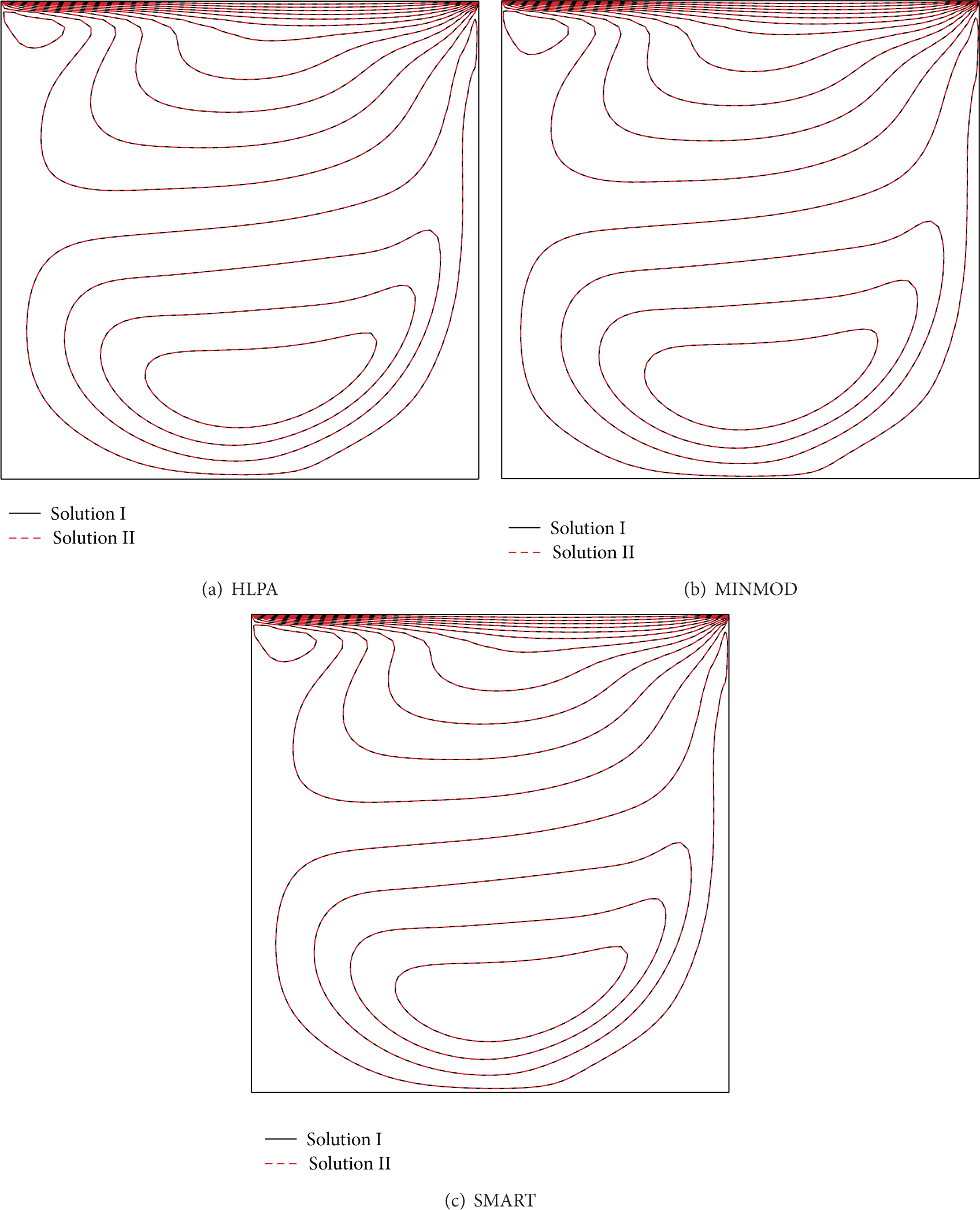
Comparison of results for two implementation methods.

Although the convergence processes of two implementation methods are different, the calculation shows that the profiles obtained by the two implementation methods of HR schemes are the same in any location of the computational domain when the calculation reaches convergence, and every segment of composite schemes has been carried out by both implementation methods during the solution process, for example the percentage of the adoption of the segment ${\tilde{\varphi }}_f={\tilde{\varphi }}_C$ in the outer domain is at least 1.6%. It can be seen from comparison and deviation that the results of the two implementation methods agree well. Similarly, it can be indicated that the deviation of the two implementation methods in this problem is caused by round-off error. In addition, it can be seen from (18) that velocity field is calculated by non-linear equations and that of temperature field is solved by linear equation, and the results of velocity field and temperature field by two implementation methods agree well respectively, so it indicates that two implementation methods of HR schemes can get same results no matter whether it is a non-linear problem or a linear problem. Therefore, the application of the two implementation methods has the same effect.

From the above two test examples it can be concluded that the adoption of DC method and the combination of SUD scheme and CD scheme to interpolate the cell face value respectively can obtain the same results as expected, which means the results obtained by the two implementation methods of HR schemes are of the same order of accuracy, and thus the two implementation methods of HR schemes are proved to be equivalent. The expression used in the first implementation method is (12), which is expressed by the two schemes that have second-order accuracy, thus the numerical solution is certain to have second-order accuracy when (12) is used. Moreover, every segment of composite scheme is presented in the form of (12), and it can be known from the equivalence of two implementation methods that the segments of composite schemes that don't pass through node Q, such as ${\tilde{\varphi }}_f={\tilde{\varphi }}_C$ and ${\tilde{\varphi }}_f=3{\tilde{\varphi }}_C$ , and the line of which is curved rather than straight, such as ${\tilde{\varphi }}_f={\tilde{\varphi }}_C(2-{\tilde{\varphi }}_C)$ , have second-order accuracy as well.

3.2. Richardson Extrapolation

Through the two different implementation methods of HR schemes employed to obtain cell face value, it has been verified in the last section that the two implementation methods are equivalent, and then verified that HR schemes satisfying the BAIR condition have second-order accuracy on the whole. In this section, order of accuracy of HR schemes is explained by Richardson extrapolation [11] combined with numerical experiments. The Richardson extrapolation can estimate the order of truncation error of the discretized equation, and its idea is:

1. Numerical computation would be carried out on three sets of grids with different densities, and the ratio between two adjacent grid systems is 3.

2. The value of ϕ in the same location of three sets of grids should be recorded.

3. The order of accuracy of truncation error is.

   $n=\frac{\ln \left[\left({\phi }_{\mathrm{3}h}-{\phi }_{\mathrm{9}h}\right)/\left({\phi }_h-{\phi }_{\mathrm{3}h}\right)\right]}{\ln \left(\mathrm{3}\right)},$

   (20)

where ϕ _h , ϕ_3h, and ϕ_9h represent the numerical solution of the grids with step size of h, 3h and 9h respectively; the value of n is the order of accuracy, for example n = 2 means that the order of truncation error is second. Three sets of grids are shown in Figure 10, node P is the communal node of three sets of grids, and symbols e_9h, e_3h and e _h represent the east face of control volume of node P in coarse grid, middle grid and refined grid respectively; s_9h, w_9h and n_9h represent the south face, west face and north face of control volume of node P in the coarse grid respectively. The numerical computation is carried out in three sets of grids respectively, if the schemes used to interpolate the value of east face of control volume of communal node P in coarse grid, middle grid and refined grid respectively are the same, (20) can be used to solve n. Meanwhile variables ϕ _h ,ϕ_3h, and ϕ_9h in (20) refer to the value of ϕ on the communal node, such as node P, calculated in three sets of grids respectively.

Figure 10:

Three sets of uniform grid systems.

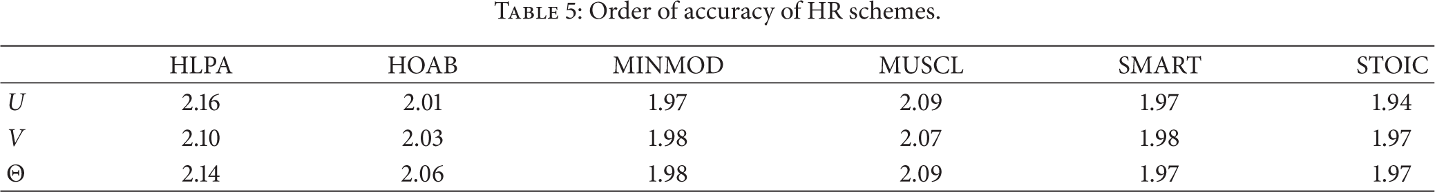
The Richardson extrapolation will be employed in the test example 2 to estimate the order of accuracy of HR schemes, and DC method will be used for the computation. The control volume number of three sets of grids are 98 × 98 (the coarse grid), 290 × 290 (the middle grid) and 866 × 866 (the refined grid) respectively. And convergence criteria for both the coarse grid and the middle grid are RES < 10⁻¹⁰, and that for the refined grid is RES < 10⁻¹³. The results of the estimation for the overall order of accuracy of schemes (the value of n) are shown in Table 5, and those of the segments of composite schemes are presented in Table 6, where the data in parentheses represent the adoption percentage of every segment of composite scheme used to interpolate the value of e_9h of control volume when computing ϕ in coarse grids. And what shown in Table 5 are the averaged results extrapolated by all nodes, which means it is neglected whether the schemes used to interpolative east face of communal node in different girds are the same or not. In Table 6, in order to satisfy the requirement (the value of ϕ in the same location) of Richardson extrapolation, for those segments whose available nodes are not enough, such as ${\tilde{\varphi }}_f=2{\tilde{\varphi }}_C,\mathrm{\hspace{0.17em}\hspace{0.17em}}{\tilde{\varphi }}_f=1$ and ${\tilde{\varphi }}_f={\tilde{\varphi }}_C$ of MUSCL, aggregation measures have been taken, that is the Richardson extrapolation has been adopted to estimate the overall order of accuracy of these segments. Moreover, in Table 6, in the process of temperature field calculation using HLPA in three sets of grids respectively, the communal nodes used in the expression ${\tilde{\varphi }}_f={\tilde{\varphi }}_C$ to interpolate the cell face value of e_9h, e_3h and e _h simultaneously are not available, thus the Richardson extrapolation can't be employed for this segment; the estimation result of order of accuracy for the QUICK segment of composite scheme is second-order, that is because only the scheme used to interpolate the east face of control volume has been concerned. However, the value of ϕ used in extrapolation also depends on the way of interpolation for south face, west face and north face, for example, if the other three faces values have been interpolated by schemes which have second-order accuracy, then it can greatly affect the accuracy of numerical solution, which can lead to the estimation result of order of accuracy for QUICK isn't equivalent to third-order. In addition, the diffusion term is discretized by CD scheme, which is second-order accurate and can also affect the value of n.

Table 5:

Order of accuracy of HR schemes.

	HLPA	HOAB	MINMOD	MUSCL	SMART	STOIC
U	2.16	2.01	1.97	2.09	1.97	1.94
V	2.10	2.03	1.98	2.07	1.98	1.97
Θ	2.14	2.06	1.98	2.09	1.97	1.97

Table 6:

Order of accuracy and percentage of segments of HR schemes.

HR Scheme	${\tilde{\mathrm{\varphi }}}_f$	n (%)
		U	V	Θ
MINMOD	${\tilde{\mathrm{\varphi }}}_f={\tilde{\mathrm{\varphi }}}_C$	2.31 (2.41%)	1.88 (2.04%)	1.97 (1.57%)
	${\tilde{\mathrm{\varphi }}}_f=\mathrm{1.5}{\tilde{\mathrm{\varphi }}}_C$	1.95 (49.05%)	1.97 (51.92%)	1.99 (52.41%)
	${\tilde{\mathrm{\varphi }}}_f=\mathrm{0.5}+\mathrm{0.5}{\tilde{\mathrm{\varphi }}}_C$	1.97 (48.54%)	1.98 (46.04%)	1.98 (46.02%)
MUSCL	$\{\begin{array}{c}{\tilde{\mathrm{\varphi }}}_f=\mathrm{2}{\tilde{\mathrm{\varphi }}}_C\\ {\tilde{\mathrm{\varphi }}}_f=\mathrm{1}\\ {\tilde{\mathrm{\varphi }}}_f={\tilde{\mathrm{\varphi }}}_C\end{array}$	2.05 (5.81%)	2.14 (4.23%)	2.08 (3.28%)
	${\tilde{\mathrm{\varphi }}}_f=\mathrm{0.25}+{\tilde{\mathrm{\varphi }}}_C$	2.10 (94.82%)	2.06 (95.77%)	2.09 (96.72%)
SMART	$\{\begin{array}{c}{\tilde{\mathrm{\varphi }}}_f=\mathrm{3}{\tilde{\mathrm{\varphi }}}_C\\ {\tilde{\mathrm{\varphi }}}_f=\mathrm{1}\\ {\tilde{\mathrm{\varphi }}}_f={\tilde{\mathrm{\varphi }}}_C\end{array}$	2.13 (4.22%)	1.99 (3.42%)	1.97 (2.35%)
	${\tilde{\mathrm{\varphi }}}_f=\mathrm{0.375}+\mathrm{0.75}{\tilde{\mathrm{\varphi }}}_C$	1.97 (95.78%)	1.97 (96.58%)	1.97 (97.65%)
STOIC	$\{\begin{array}{c}{\tilde{\mathrm{\varphi }}}_f=\mathrm{3}{\tilde{\mathrm{\varphi }}}_C\\ {\tilde{\mathrm{\varphi }}}_f=\mathrm{1}\\ {\tilde{\mathrm{\varphi }}}_f={\tilde{\mathrm{\varphi }}}_C\end{array}$	2.06 (4.57%)	1.94 (3.78%)	1.98 (2.5%)
	${\tilde{\mathrm{\varphi }}}_f=\mathrm{0.5}+\mathrm{0.5}{\tilde{\mathrm{\varphi }}}_C$	1.93 (47.74%)	1.99 (43.72%)	1.98 (51.75%)
	${\tilde{\mathrm{\varphi }}}_f=\mathrm{0.375}+\mathrm{0.75}{\tilde{\mathrm{\varphi }}}_C$	1.95 (47.69%)	1.96 (52.50%)	1.95 (45.75%)
HOAB	$\{\begin{array}{c}{\tilde{\mathrm{\varphi }}}_f=\mathrm{3.5}{\tilde{\mathrm{\varphi }}}_C\\ {\tilde{\mathrm{\varphi }}}_f=\mathrm{1}\\ {\tilde{\mathrm{\varphi }}}_f={\tilde{\mathrm{\varphi }}}_C\end{array}$	2.16 (4.70%)	2.05 (3.71%)	2.06 (2.86%)
	${\tilde{\mathrm{\varphi }}}_f=\mathrm{0.5}+\mathrm{0.5}{\tilde{\mathrm{\varphi }}}_C$	1.98 (48.18%)	2.06 (43.78%)	2.06 (51.84%)
	${\tilde{\mathrm{\varphi }}}_f=\mathrm{0.25}+{\tilde{\mathrm{\varphi }}}_C$	2.04 (47.12%)	2.01 (52.51%)	2.06 (45.30%)
HLPA	${\tilde{\mathrm{\varphi }}}_f={\tilde{\mathrm{\varphi }}}_C(\mathrm{2}-{\tilde{\mathrm{\varphi }}}_C)$	2.16 (97.59%)	2.09 (97.95%)	2.14 (98.41%)
	${\tilde{\mathrm{\varphi }}}_f={\tilde{\mathrm{\varphi }}}_C$	2.38 (2.41%)	1.95 (2.05%)	— (1.59%)

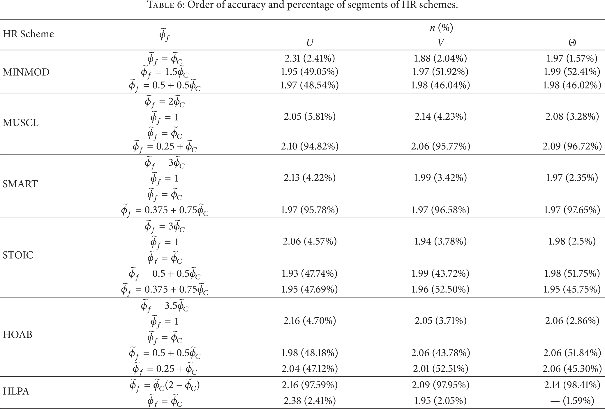
From Table 5, it is noted that the values of n representing order of accuracy of different HR schemes all equal 2 approximately; Table 6 shows that the values of n for each segment of HR schemes are also 2 approximately. Then it can be concluded that the above kinds of HR schemes possess not only second-order accuracy on the whole, but also have at least second-order accuracy of each segment, especially in the situation that ${\tilde{\varphi }}_f={\tilde{\varphi }}_C$ or ${\tilde{\varphi }}_f=3{\tilde{\varphi }}_C$ and the type of characteristic line is curved.

4. Conclusions

The numerical solutions gained by DC method and the combination of two schemes possessing second-order accuracy respectively have been compared when HR schemes is used to discretize the governing equation. And it has been verified that HR schemes satisfying the BAIR condition have at least second-order accuracy (no matter whether the lines of which are straight or curved). In other words, any scheme of which the line in the NVD lies between the lines of two second-order schemes (SUD scheme and CD scheme) in the inner domain and happens to coincide with FUD scheme in the outer domain dose possesses at least second-order accuracy. The following points should be valued particularly:

1. For ${\tilde{\varphi }}_f={\tilde{\varphi }}_C$ segment, only when its line locates in BAIR region which means the line lies between SUD scheme and CD scheme, the adoption of the expression ${\tilde{\varphi }}_f={\tilde{\varphi }}_C$ has second-order accuracy, and in other region it still has first-order accuracy.

2. Those segments locating in BAIR region without passing through node Q, such as ${\tilde{\varphi }}_f=3{\tilde{\varphi }}_C$ , can be verified by Taylor expansion that they have lower-order accuracy when employed independently. However, when they are parts of composite schemes, these segments are second-order accurate as they lie in BAIR region.

3. The scheme whose line is curved and passes through node Q in BAIR region is also second-order accurate as the scheme whose line is straight.

Meanwhile, the application of Richardson extrapolation has explained and also proved the above statements. In addition, DC method is recommended to implement HR schemes because of its simplicity and superiority in computation efficiency.