On Helical Projection and Its Application in Screw Modeling

Abstract

As helical surfaces, in their many and varied forms, are finding more and more applications in engineering, new approaches to their efficient design and manufacture are desired. To that end, the helical projection method that uses curvilinear projection lines to map a space object to a plane is examined in this paper, focusing on its mathematical model and characteristics in terms of graphical representation of helical objects. A number of interesting projective properties are identified in regard to straight lines, curves, and planes, and then the method is further investigated with respect to screws. The result shows that the helical projection of a cylindrical screw turns out to be a Jordan curve, which is determined by the screw's axial profile and number of flights. Based on the projection theory, a practical approach to the modeling of screws and helical surfaces is proposed and illustrated with examples, and its possible application in screw manufacturing is discussed.

1. Introduction

Projection, or three-dimensional (3D) projection, is a general method of mapping space points to a 2D plane. Since its invention, this method has been widely used for graphic representation and solution of space problems in engineering. Although the advent of computers makes it obsolete to solve space problems manually by the geometrical projection protocols, this method finds even more applications in contemporary engineering, especially in computer graphics, computer aided design and manufacturing (CAD/CAM) systems, and any other systems that require graphical visualization.

Conventionally, the projection, either orthographic or perspective, is produced by rays of imaginary straight lines. While it proves prestigious in most cases, the weakness of this method was also detected with respect to curved surfaces. Therefore, Tevlin [1] proposed the use of cylindrical helixes in projection, which brought about a new type of projection, namely, helical projection. In his work, he also demonstrated the new method with respect to the solution of a number of geometrical problems pertinent to helixes and helical surfaces.

Screws are a typical category of components that capitalize on helical surfaces. In addition to those used as threaded fasteners, there are also many discrete screws in the form of conveyors, compressor rotors, extruders, helical gears, helical ball bearing, or augers, and so forth (hereinafter these helical components are all referred to as screws). Vary as these screws may, they all need their helical surfaces well-tailored to the particular need of the associated machine [2]. Their shape and accuracy have a profound impact on the quality of product [3, 4].

As these screws or screw-shaped components, in all their many and varied forms, are finding wider and wider application in industry along with the ever increasing demand for higher quality and lower cost, more and more attention has been drawn to their modeling and manufacture [5, 6]. Focusing on the generation of the helical surface profiles on cutting tools, Sun et al. [7] presented a simulation model for the grinding process of these helical surfaces. Ilie and Subic [8] proposed a parametric 3D geometric model of twin-screw supercharger rotors. Kawalec and Wiktor [9] developed a method for geometric modeling of the mating teeth of helical gears. Adair et al. [10] put forward a way for economical manufacture of an aerostatic lead screw. In these investigations, the geometrical models are usually created with respect to the particular components and processes. Considering the possible application of new processes in this domain, a common approach for modeling the category of components is highly desired.

In parallel, the numerical nature of geographical projection was revealed [11]. Using transformation matrices, any type of 3D projection can be generated by computers. This makes the projection methods not only means of visualization or graphic representation but also a way for modern computer systems to solve design and manufacturing problems [12, 13]. The ever-increasing use of computers in industry also entails new data models for efficiently manipulating and communicating product information [14]. Although the pursuit of a seamless integration of CAD/CAPP/CAM/CNC systems over the last decades has led to a number of new paradigms for product representation [15], those components with helical structures have been seldom addressed. Currently, prismatic and cylindrical components have been well defined in the STEP-NC standard (ISO 14649) based on manufacturing features. However, it is not the case for helical components except for simple threads. Among others, a major reason is the lack of a comprehensive data model for this particular category of components. To this end, it is highly desired to find out a uniform and feature-based approach to describing the whole screw part (not just the helical grooves or ridges), whether it is an extruder screw, compressor rotor, or in any other form. On this background, this paper aims to identify the characteristics of the helical projection method and explore its use in geometric modeling of helical components focusing on screws.

2. Helical Projection

2.1. Overview

In helical projection as proposed by Tevlin, cylindrical helixes with a common axis and identical pitch are used as projection lines. A plane either incident to or perpendicular to the axis is taken as projection plane, as shown in Figure 1. For any point P, there is one and only one helix passing through it, and the intersection point of the helix with the plane is called the projection of point P. So any point P can be defined by two helical projections (p¹ and p²) together with a supplementary parameter (φ, e.g.).

Figure 1:

Helical projection proposed by Tevlin.

Although the two projections prove to be useful in solving geometrical problems, they are actually correlated. Once the helixes and projection planes are chosen, either p¹ or p² will lead to the construction of the other. Thus in this paper we will only consider the projection plane perpendicular to the helical axis, and the main focus will be on the theoretical model, characteristics, and potential application in component modeling.

2.2. Mathematical Representation of the Projection Lines

A helix is often modeled as the trajectory of a moving point. In the Cartesian coordinate system OXYZ as shown in Figure 2, assuming that the helix is produced by a point that moves along the z axis at a constant speed, starting from the XOY surface, then, the parametric equation of the helix can be written as

$\begin{array}{l}x\left(t\right)={\rho }_{\mathrm{0}}\cos \left(\omega t+{\phi }_{\mathrm{0}}\right),\\ y\left(t\right)={\rho }_{\mathrm{0}}\sin \left(\omega t+{\phi }_{\mathrm{0}}\right),\\ z\left(t\right)=vt,\end{array}$

(1)

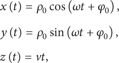
where ρ₀ is its radius, φ₀ is its initial angle with respect to the XOY plane, ω and v are the speeds at which the point rotates around and moves along the z axis, respectively, and ω,v≠0.

Figure 2:

Helix and its parameters.

Let s be the lead (pitch) of the helix, positive for right-handed and negative for left-handed (in practice, the lead is usually defined as the absolute value; in this paper however, it is allowed to be negative for unified representation of helixes), then

$s=\frac{\mathrm{2}\pi v}{\omega }.$

(2)

In this way, any helix defined by (1) and shown in Figure 2 can be represented as Γ(s,φ₀,ρ₀). If s sticks to a fixed value and φ₀ varies in domain (0 ≤ φ₀ < 2π) and ρ₀ in (0 < ρ₀ < ∞), then Γ(s,φ₀,ρ₀) stands for any helix that shares the same axis, pitch, and handedness. The totality of these helixes, noted as Ωs:{Γ(s,φ₀,ρ₀) ∣ 0 ≤ φ₀ < 2π,0 < ρ₀ < ∞}, is referred to hereinafter as the projection lines. Obviously, they are parallel and pass any point in the Cartesian space.

Please note that all parameters of the projection lines are kept irrelevant to Z coordinate to guarantee their parallelism. In theory, however, they may vary with the Z coordinate in a controlled way.

2.3. Projective Transformation

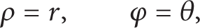
As shown in Figure 3, assume P(x,y,z) to be an arbitrary point in the Cartesian space, through which Γ(s,φ₀,ρ₀) passes. According to (1) and (2), there is

$x={\rho }_{\mathrm{0}}\cos \left(\frac{\mathrm{2}\pi z}{s}+{\phi }_{\mathrm{0}}\right),\hspace{1em}\hspace{1em}y={\rho }_{\mathrm{0}}\sin \left(\frac{\mathrm{2}\pi z}{s}+{\phi }_{\mathrm{0}}\right).$

(3)

Figure 3:

Coordinate system and calculation for helical projection.

Suppose the projection plane π is positioned through O′(0,0,Z₀) and perpendicular to the z axis and the projection of P(x,y,z) on the plane is p′(x′,y′) in the O′X′Y′ coordinate system, then there exists

$x^{\prime }={\rho }_{\mathrm{0}}\cos \left(\frac{\mathrm{2}\pi z_{\mathrm{0}}}{s}+{\phi }_{\mathrm{0}}\right),\hspace{1em}\hspace{1em}{y}^{\prime }={\rho }_{\mathrm{0}}\sin \left(\frac{\mathrm{2}\pi z_{\mathrm{0}}}{s}+{\phi }_{\mathrm{0}}\right).$

(4)

Combination of (3) and (4) leads to

$x^{\prime }=x\cos \varphi -y\sin \varphi ,\hspace{1em}\hspace{1em}{y}^{\prime }=x\sin \varphi +y\cos \varphi ,$

(5)

where ϕ = 2π(Z₀ − z)/s.

If cylindrical coordinates (ρ,φ,z) are substituted for P(x,y,z) and polar coordinates (ρ′,φ′) for p′(x′,y′), then (5) can be rewritten as

${\rho }^{\prime }=\rho ,\hspace{1em}\hspace{1em}{\phi }^{\prime }=\phi +\frac{\mathrm{2}\pi \left(Z_{\mathrm{0}}-z\right)}{s}.$

(6)

Equation (6) indicates that the helical projection is a combination of orthogonal projection and an additional rotation. The rotation depends on the distance between the object and the projection and the lead of the projection lines. In case s → ∞, it will degrade into orthogonal projection, and, in case s = 0, there will be no projection (these special cases are ignored herein unless otherwise specified).

2.4. Projective Properties

Although the projection of any object can be obtained through the use of (5) or (6), it can also be predicted in some cases without the aid of mathematical calculation. To this end, a number of properties inherent to the helical projection are outlined, with respect to particular lines and surfaces as follows (please note that the term view is also used hereinafter to refer to the result of projecting from an object onto a projection plane, though the view in this instance may differ significantly from the picture of the object as seen with lines of sight).

Property 1. For fixed lines and plane of projection, the rotation angle of the view is in proportion of the distance between the object and the projection plane.

Property 2. If the object moves a multiple of |s| nearer to or farther from the projection plane, the view appears the same.

Property 3. Cylindrical helixes and helical surfaces parallel to the projection lines are projected to points and curves, respectively.

Property 4. A line segment in parallel to the axis is projected to a circular arc in the view.

Suppose there is a straight line which satisfies

$\rho =r,\hspace{1em}\hspace{1em}\phi =\theta ,$

(7)

where r and θ are invariables.

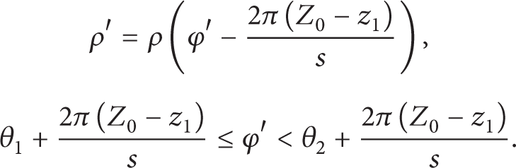
According to (6), the view of the line can be expressed as

${\rho }^{\prime }=r,\hspace{1em}\hspace{1em}{\phi }^{\prime }=\theta +\frac{\mathrm{2}\pi \left(Z_{\mathrm{0}}-z\right)}{s}.$

(8)

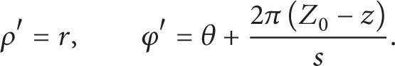
So the view of the line would be an arc which centers on the origin of the projection plane, with a radius of r, and a central angle of |2π(z₂ − z₁)/s|, starting from θ + 2π(Z₀ − z₁)/s and ending at θ + 2π(Z₀ − z₂)/s. If the line is longer than the lead of the projection lines, that is, |z₂ − z₁| ≥ s, the view would be a complete circle. Exception occurs if the line coincides with the axis. In this case, the view would be just a point at the origin of the projection plane.

Property 5. A straight line which intersects the axis at an oblique angle is projected to an Archimedean spiral in the view.

Suppose there is a straight line which satisfies

$\rho =az+b,\hspace{1em}\hspace{1em}\phi =\theta ,$

(9)

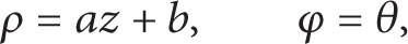
where a,b,θ are invariables, and a≠0.

According to (6), the view of the line can be expressed as

${\rho }^{\prime }=az+b,\hspace{1em}\hspace{1em}{\phi }^{\prime }=\theta +\frac{\mathrm{2}\pi \left(Z_{\mathrm{0}}-z\right)}{s}.$

(10)

After z being eliminated, it leads to

${\rho }^{\prime }=a^{\prime }{\phi }^{\prime }+b^{\prime },$

(11)

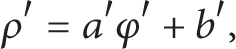
where a′ = − (as/2π) and b′ = aZ₀ + b − a′θ.

Property 6. A straight line which is skew but not perpendicular to the axis is projected to the involute of a circle.

Suppose there is a straight line which satisfies

$x=az+b,\hspace{1em}\hspace{1em}y=c,$

(12)

where a,b,c are invariables, and a≠0.

According to (5), the view of the line can be expressed as

$\begin{array}{l}{x}^{\prime }=\left(a^{\prime }\varphi +b^{\prime }\right)\cos \varphi -c\sin \varphi ,\\ y^{\prime }=\left(a^{\prime }\varphi +b^{\prime }\right)\sin \varphi +c\cos \varphi ,\end{array}$

(13)

where a′ = − (a·s/2π) and b′ = a·Z₀ + b.

Obviously, (13) stands for the involute of a circle with radius c. If we let c = 0, then it will degrade to an Archimedean spiral.

Property 7. Any plane curve parallel to the projection plane is shown, though rotated an angle, in its true size and shape in the view.

Suppose there is an arbitrary curve on plane F1:z = z₁, which is parallel to the projection plane; then the curve can be expressed as

$\rho =\rho \left(\phi \right),\hspace{1em}\hspace{1em}{\theta }_{\mathrm{1}}\le \phi <{\theta }_{\mathrm{2}},\hspace{1em}\hspace{1em}z=z_{\mathrm{1}}.$

(14)

According to (6), the view of the curve can be specified in polar coordinates as

$\begin{array}{c}{\rho }^{\prime }=\rho \left({\phi }^{\prime }-\frac{\mathrm{2}\pi \left(Z_{\mathrm{0}}-z_{\mathrm{1}}\right)}{s}\right),\\ {\theta }_{\mathrm{1}}+\frac{\mathrm{2}\pi \left(Z_{\mathrm{0}}-z_{\mathrm{1}}\right)}{s}\le {\phi }^{\prime }<{\theta }_{\mathrm{2}}+\frac{\mathrm{2}\pi \left(Z_{\mathrm{0}}-z_{\mathrm{1}}\right)}{s}.\end{array}$

(15)

Based on Property 7, the following inferences are drawn.

Inference 1. Any plane surface with definite boundaries is shown in its true size and shape (ignoring the rotation) in the view.

Inference 2. Any circular arc perpendicular to the axis is projected to a circular arc of the same size.

Inference 3. A straight line perpendicular to the axis is projected to a straight line of the same length. In particular, if it intersects the axis, its view passes through the origin of the projection plane.

Inference 4. A cylindrical surface coaxial with the projection lines is projected to a complete circle of the same radius.

3. Helical Projection of Screws

3.1. Overview

The helical projection (view) of a screw or any other 3D object is a combination of the projections of all its surfaces. For a screw as shown in Figure 4(a), which comprises a number of helical surfaces and two planes, a view as shown in Figure 4(b) may be obtained by projecting it using the projection lines Ωs (s equals the screw lead) onto a plane such as its end face (the XOY plane). In the view, the arcs ab and cd are projections of the flat portions at the ridge and the bottom, respectively, and the segments bc and ad are those of the slopes. The whole view constructs a closed area, which shows the true shape of both ends of the screw. With respect to screws like this, it is secure to say the following.

Figure 4:

Helical projection of an example screw.

Inference 5. The helical projection of a screw is a simple closed curve (Jordan curve) congruent to a cross-section of the screw.

Inference 6. For a screw longer than its lead, the projection of its axial profile within one lead's length equals that of its full length.

3.2. Axial Form

For such a screw as shown in Figure 4(a), assuming its axial profile is depicted as y = f(z), 0 ≤ z < s, then, any point on the profile can be expressed as P(0,y,z) in the Cartesian coordinate system.

Let the projection plane pass point O, the origin of the coordinate system, and let the projection of point P be denoted as p′(ρ′,φ′) in the polar coordinate system.

If y ≥ 0, then P(0,y,z) is equivalent to P(0,y,z) in cylindrical system that corresponds to the Cartesian system. According to (4), there is

${\rho }^{\prime }=y,\hspace{1em}\hspace{1em}{\phi }^{\prime }=\frac{\mathrm{2}\pi z}{s}.$

(16)

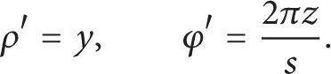
Substitute y = f(z) into the equation and we get

${\rho }^{\prime }=f\left(\frac{s}{\mathrm{2}\pi }{\phi }^{\prime }\right),\hspace{1em}\mathrm{0}\le {\phi }^{\prime }<\mathrm{2}\pi .$

(17)

Otherwise if y < 0, P(0,y,z) is equivalent to P(− y,π,z). Equation (17) holds true in this case because the polar coordinates (− ρ,π + φ) and (ρ,φ) refer to the same point.

Based on Inference 6 and (17), the following statement may be inferred.

Inference 7. If a screw's helical projection is depicted by a mathematical equation using polar coordinates, its axial profile can be expressed by a similar equation using Cartesian coordinates.

This is useful in predicting a screw's helical projection. For example, if the flank of the helical ridge takes the shape of a parabola (y = ax² + bx + c in the OXYZ system, where a, b, and c are constants), then the corresponding helical surface would be projected to a curve on the XOY plane, which satisfies ρ′ = a(sφ′/2π)² + b(sφ′/2π) + c.

3.3. Multistart Screws

For a multistart crew, whose number of starts is n and whose pitch is p(p > 0), there exists

$s=\pm np.$

(18)

Let C₁ stand for the segment of its axial profile within the first pitch, which is depicted as

$y=f\left(z\right),\hspace{1em}\mathrm{0}\le z<p.$

(19)

Then, the segment within the kth pitch (C _k ,1 < k ≤ n) can be expressed as

$y=f\left(z+\left(k-\mathrm{1}\right)p\right),\hspace{1em}\mathrm{0}\le z<p.$

(20)

As the segments are of the same geometry, there is

$f\left(z+\left(k+\mathrm{1}\right)p\right)=f\left(z\right).$

(21)

Let the projection plane coincide with the XOY and let c₁′(ρ₁′,φ₁′) be the projection of C₁ and c _k ′(ρ _k ′,φ _k ′) of C _k . It is not hard to prove the following relationship:

$\begin{array}{l}{\rho }_k^{\prime }={\rho }_{\mathrm{1}}^{\prime },\\ {\phi }_k^{\prime }={\phi }_{\mathrm{1}}^{\prime }\mp \frac{\mathrm{2}\pi \left(k-\mathrm{1}\right)}{n},\end{array}$

(22)

$\begin{array}{c}{\rho }_k^{\prime }=f\left(\frac{np}{\mathrm{2}\pi }\left({\phi }_k^{\prime }\pm \frac{\mathrm{2}\left(k-\mathrm{1}\right)\pi }{n}\right)\right),\\ \frac{\mathrm{2}\left(k-\mathrm{1}\right)\pi }{n}\le \pm {\phi }_k^{\prime }<\frac{\mathrm{2}k\pi }{n},\end{array}$

(23)

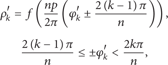
where “+” is for right-handed and “−” for left-handed screws, respectively. Equation (23) suggests the following.

Inference 8. The projection of an n-start screw appears as a pattern of n repetitions.

By way of illustration, Figure 5 shows the projections of a square thread screw having one Figure 5(a), two Figure 5(b), three Figure 5(c), and four Figure 5(d) starts, respectively.

Figure 5:

The projection of the single-start and multiple-start screws.

4. Potential Application and Discussion

4.1. Screw Modeling Based on Helical Projection Theory

By means of helical projection as stated above, space objects like helical surfaces and screws can be mapped into 2D elements. This provides the foundations for description and representation of those objects. Nevertheless, the reverse process can also be used to construct helical objects based on plane curves.

Generally, a piece of curve can be described in polar coordinates as

${\rho }^{\prime }={\rho }^{\prime }\left({\phi }^{\prime }\right).$

(24)

Suppose it is produced by projecting a cylindrical helical surface onto the XOY plane. Combine (6) and (22) and set Z₀ to 0; we can get the equation of the helical surface as follows:

$\rho ={\rho }^{\prime }\left(\phi -\frac{\mathrm{2}\pi }{s}·z\right).$

(25)

Equations (24) and (25) indicate a rather easy way for esTablishing and representing a cylindrical helical surface. In particular, if the 2D curve is closed and does not intersect itself, a screw would be created using the same formula. Table 1 lists some examples of the 2D curves and corresponding helical surfaces. As illustrated in the table, any particular kind of helical surface can be generated through a specified curve, and a screw is constructed if the curve (either a smooth curve or a composite curve of class C⁰) is closed.

Table 1:

Curves and corresponding helical surfaces.

The approach can also be generalized for screws with variable pitch and diameters. Suppose the radius and the lead of a screw both vary with the Z coordinate. Let r = r(z) represent the major radius and s = s(z) the lead of the screw. Then the helical surfaces of the screw created using the curve as depicted by (24) must satisfy the following equation:

$\rho =\frac{r\left(z\right)}{r\left(\mathrm{0}\right)}·{\rho }^{\prime }\left(\phi -\mathrm{2}\pi {{\displaystyle \int }}_{\mathrm{0}}^z\frac{dz}{s\left(z\right)}\right),$

(26)

where r(0) is the major radius of the screw at its starting point.

4.2. Discussion

As revealed in this work, the shift from straight lines to helixes brings about some interesting characteristics to the projection method, which in turn provides an alternative and more efficient way for modeling helical components. Although further study is still needed to put it into practice, it is evident that the helical projection method does have advantages in describing the feature of complex helical surfaces. For example, a cylindrical screw, no matter how many flights it has and how complex its grooves and ridges are, would be projected into a closed curve, which reflects the features of all its surfaces. Based on this, any cylindrical screw can be defined geometrically by its helical projection and a couple of additional parameters including length, pitch, and handedness.

This method may also find application in the manufacture of this kind of components. For example, the screw model may be utilized in additive manufacturing to calculate the two-dimensional layers of a complex compressor rotor. In addition, the proposed approach also provides an alternative way for validating the tool path for these components. Conventionally, before the real machining, the tool location needs to be checked by calculating the 3D relationship between the tool and the helical surfaces. The validation could involve huge computation and be very time-consuming if the helical surfaces are complex. Based on the work of this paper, however, both the component and the cutter can be easily converted to 2-dimensional curves. So the validation can be done by just checking the relationship between the projected curves.

5. Conclusion

In the light of the need to overcome the weakness of conventional projection methods in solving engineering problems associated with helical surfaces, this paper investigated the helical projection method focusing on its projective properties and potential use in component modeling and representation. The main work can be concluded as follows.

1. This paper investigated the numerical nature of the helical projection and identified a number of projective properties inherent to the method with respect to straight lines, curves, and planes in different positions, which are useful in determining the helical views of a space object.

2. This paper looked into the characteristics of screws’ helical projection. The result showed that the helical view of a screw is a simple closed curve. The curve does not only reflect the number of flights and the cross-section of the screw, but also is of the same function type as the axial section profile, provided the former is depicted in polar coordinates and the latter in Cartesian coordinates.

3. The paper also explored possible application of the helical projection theory in screw modeling. The result showed that screws or their helical surfaces can be constructed in a pretty easy way based on Jordan curves, which are considered as their helical projections. This also provides a workable way for feature-based description of screws and screw-like components. Further study will follow to capitalize on the method and put it into practice. In consideration of the variety of screws, future work will also be directed at its particular applications with respect to screws with variable pitches and diameters.

Conflict of Interests

The authors declare that there is no conflict of interests regarding the publication of this paper.