Sage Journals: Discover world-class research

Abstract

This paper develops an efficient and distributed boundary detection algorithm to precisely recognize wireless sensor network (WSN) boundaries using only local connectivity information. Specifically, given any node in a WSN, the proposed algorithm constructs its 2-hop isocontour and locally makes a rough decision on whether this node is suspected to be on boundaries of the WSN by examining the associated 2-hop isocontour. Then, a heuristic operation is performed to refine this decision, with the result that the suspected boundary node set is significantly shrunk. Lastly, tight boundary cycles corresponding to both inner and outer WSN boundaries are derived by searching the suspected boundary node set. Furthermore, regarding WSNs with relatively low node densities, the proposed algorithm is adapted to improve the quality of boundary detection. Even though the proposed algorithm is initially presented under the assumption of the idealized unit disk graph (UDG) model, we further consider the more realistic quasi-UDG (QUDG) model. In addition, a message complexity analysis confirms the energy efficiency of the proposed algorithm. Finally, we carry out a thorough evaluation showing that our algorithm is applicable to both dense and sparse deployments of WSNs and is able to produce accurate results.

1. Introduction

Wireless sensor networks (WSNs), comprised of hundreds or thousands of small and inexpensive (sensor) nodes with constrained computing power, limited memory, and short battery lifetime, can be used to monitor and collect data in a region of interest [1]. Given a WSN, nodes on or near boundaries normally play a more important role than the other nodes. First, these nodes directly interact with the outside environment, such as events entering or leaving the region monitored by the WSN [2–4] and any communication with the outside environment [5]. Second, these nodes help to extract further information about the WSN structure which is useful for routing, guiding, and management purposes [6–10]. Third, due to the correspondence between the boundaries of a WSN and its physical environment, such as a building floor plan, a map of a transportation network, terrain variations, and obstacles (buildings, lakes, etc), these nodes are important for keeping track of the WSN shape which indicates significant features of the underlying environment [11, 12]. Last but not least, in contrast to the outer boundary of a WSN, inner boundaries denote boundaries of inner holes of the WSN and are important indicators of the general health of a WSN, such as insufficient coverage and connectivity [13, 14]; for instance, identifying inner boundaries reveals groups of destroyed sensors due to physical destruction or power depletion, where additional sensor deployment is needed [15]. Therefore, boundary detection is of great importance for various WSN applications, such that considerable efforts have been invested in the development of boundary detection algorithms [16–35].

In this paper, we focus on detecting WSN boundaries by making use of only low-cost connectivity information between neighboring nodes and develop an efficient and distributed algorithm precisely discovering both inner and outer boundaries. At the beginning, we assume that wireless communications satisfy the idealized unit disk graph (UDG) model, where two nodes are connected by an edge if and only if their distance is at most $1$ . Like the approaches in [20, 26, 30], our approach is also inspired by the feature that isocontours constructed in terms of the minimal hop counts from a root node are broken by boundaries or holes. Specifically, given a WSN with a sufficiently high node density, the proposed algorithm utilizes only 3-hop neighboring node information to construct $2$ -hop isocontour of each node and roughly decides whether each node is suspected to be a boundary node or not; then, a heuristic operation based on message exchanges between neighboring nodes is introduced to refine these decisions and significantly shrinks the suspected boundary node set; lastly, tight boundary cycles corresponding to both inner and outer boundaries of the WSN are obtained by searching the suspected boundary node set in a distributed fashion and provide much valuable knowledge to various WSN applications. Additionally, a message complexity analysis indicates that the proposed algorithm is energy efficient. More importantly, we address two practical issues in relation to applying our algorithm in realistic scenarios, for example, where the node density of a WSN is not sufficient and where wireless communications do not satisfy the idealized UDG model. Simulations with respect to various scenarios confirm the effectiveness of the proposed algorithm and show that the proposed algorithm is even applicable in sparse deployments of WSNs where the average node degree is as low as 9.

The remainder of this paper is organized as follows. The next section briefly reviews the literature of boundary detection. Section 3 formulates the problem of boundary detection. Section 4 describes the proposed algorithm in detail, and Section 5 discusses practical issues in relation to applying the proposed algorithm. Section 6 presents extensive simulations to confirm our results. Finally, we conclude this paper in Section 7.

2. Related Work

Normally, boundary detection algorithms can be classified into three categories: geometric, statistical, and topological methods.

Geometric methods [16, 24] use geographical location information to find nodes on boundaries. The first paper on this topic, by Fang et al. [16], assumes that the nodes know their geographical locations and that the wireless channel follows the UDG model. The definition of holes in [16] is intimately associated with geographical forwarding such that a packet can only get stuck at a node on hole boundaries. Fang et al. also proposed a simple algorithm that greedily sweeps along hole boundaries and eventually discovers boundary cycles. Though the geometric method can find more accurate boundary nodes than other two kinds of methods in a WSN, the requirement of node geometric location information limits its application, especially in large scale WSNs.

Unlike geometric methods, statistical methods [17, 19, 21, 29] usually make assumptions about the probability distribution of the node deployment. Thus, boundary nodes can be probabilistically identified based on some statistical properties under certain network conditions. Fekete et al. [17] proposed a boundary detection algorithm for sensors uniformly and randomly deployed inside a geometric region. The basic idea is that nodes on the boundaries have much lower average node degrees than nodes in the “interior” of the network. Statistical arguments yield an appropriate degree threshold to differentiate boundary nodes. By exploiting the number of 2-hop neighbor nodes, Chen et al. [29] proposed an algorithm with a significant improvement in boundary recognition contrasted with Fekete's algorithm in low-density WSNs. Another statistical approach in [19] computes the “restricted stress centrality” of a node, which measures the number of shortest paths going through this node with a bounded length. Due to the fact that interior nodes tend to have higher centralities than the nodes on the boundaries in WSNs with sufficiently high node densities, the centrality thus can be used to realize boundary detection. One major weakness of the statistical methods is the unrealistic requirement on node distribution and density (e.g., the average node degree needs to be 100 or higher in [17]). Another major weakness lies in that the criteria for identifying boundary nodes acquired from the statistical characteristics cannot guarantee finding out boundary nodes precisely.

Topological methods [18, 20, 22, 23, 25, 26, 28, 30, 31, 34] use the topological properties such as the information of connectivity to identify the boundary nodes. Normally, topological method has higher packet control overheard than the previous two methods due to having to collect information from neighboring nodes; however, it does not need location information and has better accuracy of finding boundary nodes than statistical method. Ghrist and Muhammad [18] proposed an algorithm that detects holes via homology; however, the algorithm is centralized, with assumptions that both the sensing range and communication range are disks with radii carefully tuned. Kröller et al. [22] presented a new algorithm by searching for combinatorial structures called flowers and augmented cycles; they make less restrictive assumptions on the problem setup by he quasi-UDG (QUDG) model in which two nodes are connected if their distance is below d (<1), are disconnected if above 1, and may or may not be connected if in between; the success of this algorithm critically depends on the identification of at least one flower structure, which may not always be the case especially in a sparse network.

Towards a practical solution, Funke and Klein [20] developed a simple heuristic with only connectivity information; the basic idea is to construct isocontours based on hop count from a root node and identify where the contours are broken; under the UDG model and a sufficient node density, the algorithm outputs nodes marked as boundary with certain guarantees; the simplicity of the algorithm is appealing, but the algorithm only identifies nodes that are near the boundaries and the density requirement of the algorithm is also rather high. Khan et al. [26] proposed a variant of [20] by examining the 2-hop isocontour of each node and show that if there exists a closed cycle in the 2-hop isocontour of one node, this node is an interior node, and vice versa. Another algorithm proposed by Chu and Ssu [30], similar to [26], relaxes the condition of differentiating boundary nodes from interior nodes and thus identifies more nodes as boundary nodes. Although, these algorithms are as simple as the one in [20], they have the same weakness as well, namely, requiring a high node density, identifying more nodes than actual ones, and not showing how the identified boundary nodes are connected in a meaningful way. The proposed algorithm is also based on examining isocontours of nodes in a WSN but will turn out to produce superior results in contrast to existing algorithms.

3. Problem Formulation

Suppose a large number of (sensor) nodes, say n nodes, are scattered in a 2-dimensional geometric region where nearby nodes are connected with each other to form a WSN. For ease of presentation, we assume that the wireless communications follow the UDG model. This WSN can be modeled as a graph $G (V, E)$ where the vertex set V denotes nodes and the edge set E denotes communication links between pairs of nodes. Without loss of generality, we assume the graph $G (V, E)$ is connected. Besides, we use the following mathematical notations throughout this paper. The embedding that maps the vertexes V to the actual nodes in the WSN is denoted by $p : V \to R^{2}$ ; the i-hop neighbor nodes of node $n_{x}$ is denoted by $N_{i} (n_{x})$ ; $| \cdot |$ computes the cardinality of a set.

From the geometric point of view, the outer boundary of the WSN is the minimal closed curve enclosing the graph $G (V, E)$ but not enclosing any other closed curve that encloses the graph $G (V, E)$ ; similarly, an inner boundary of the WSN is the maximal closed curve enclosing a hole of the graph $G (V, E)$ but not being enclosed by any other closed curve that encloses the same hole. Hence, an outer (or inner) boundary of the WSN is actually comprised of edges, vertices, and segments of edges in the graph $G (V, E)$ , as illustrated in Figure 1.

Figure 1

The outer and inner geometric boundaries (solid curves) of a WSN. The dashed line denotes communication links.

With the above geometric boundaries, we can readily define boundary nodes as follows. First, nodes belonging to boundaries are definitely boundary nodes. Second, if any segment is involved in a boundary, edges and nodes belonging to this boundary will not be able to form a (closed) boundary cycle corresponding to this boundary, so that extra nodes must be incorporated as boundary nodes. Existing works [22, 23] search for the shortest path between the pair of boundary nodes which are the ends of a segment or a series of connected segments of a boundary and group the nodes along the shortest path into boundary nodes. For example, nodes 1 and 2 in Figure 1 do not lie on any boundaries but are also regarded as boundary nodes so as to form boundary cycles. As opposed to boundary nodes, all the other nodes are named interior nodes. In principle, the task of boundary (and hole) detection is to identify boundary nodes and then construct corresponding boundary cycles.

As pointed out in [25], a connectivity domain description of a WSN (e.g., $G (V, E)$ ) corresponds to more than one valid embedding in physical domain, even though only one of them (e.g., p) corresponds to the physical WSN; however, it is hard to identify the correct embedding (e.g., p) solely based on the connectivity information, and, in contrast, using only connectivity information, a union of boundary nodes in every possible embedding are identified as boundary nodes and include as a subset the set of actual boundary nodes (which satisfy the aforementioned definition of boundary nodes) of the WSN.

For clarification, we call the nodes belonging to boundaries as actual boundary nodes and call the other nodes as actual interior nodes. Therefore, using given local connectivity information, our goal is to approximately discover a boundary node set, including not only actual boundary nodes but also some actual interior nodes near WSN boundaries, to try to reduce the size of the boundary node set and further to extract precise boundary cycles from the discovered boundary node set.

4. Proposed Boundary Detection Algorithm

The basic idea of the proposed algorithm is firstly identifying a set of suspected boundary nodes, then refining them, and lastly searching them for tight boundary cycles. The outline is listed below. (1)

Each node, say node $n_{0}$ , maintains a local variable, denoted by $f_{t}$ , which is initialized based on its $2$ -hop isocontour extracted from the subgraph of $G (V, E)$ induced by $n_{0}$ , $N_{1} (n_{0})$ , and $N_{2} (n_{0})$ . According to the value of $f_{t}$ , it is roughly decided whether node $n_{0}$ is a boundary node: $f_{t} = 1$ indicates that node $n_{0}$ is likely to be a boundary node and is thus termed as a suspected boundary node, while $f_{t} = 0$ indicates that node $n_{0}$ is identified to be an interior node, as shown in Figure 2(b).

(2)

After exchanging the values of $f_{t}$ between pairs of neighboring nodes, each suspected boundary node locally performs a heuristic operation to update the value of its $f_{t}$ according to the portion of identified interior nodes in its $1$ -hop neighbor nodes, namely, refining the rough decision made in the previous step, as illustrated in Figure 2(c).

(3)

Each suspected boundary node, say node $n_{0}$ , maintains another local variable, denoted by $f_{d}$ , to differentiate itself from the other suspected boundary nodes in $N_{1} (n_{0})$ in terms of proximities to boundaries; see (1) for the calculation of $f_{d}$ at node $n_{0}$ .

(4)

The suspected boundary nodes cooperatively search for boundary cycles based on their values of $f_{d}$ . As a result, a set of tight boundary cycles corresponding to inner and outer boundaries are obtained, as shown in Figure 2(d).

Figure 2

Snapshots of each step during the execution of the proposed algorithm in a WSN with the average node degree of 18.8 and with a circular hole. (a) The Node deployment in the WSN. (b) The snapshot after initializing $f_{t}$ at each node. (c) The snapshot after performing the erosion operation. (d) The snapshot after searching for boundary cycles. Dark black points denote nodes with $f_{t} = 1$ , grey points denote nodes with $f_{t} = 0$ , and red curves denote boundary cycles.

In what follows, we will describe each step of the proposed algorithm in detail. Due to the fact that the power at each node in WSNs is limited and message transmission is the main source of energy consumption, we also provide a message complexity analysis of the proposed algorithm at each step. For ease of analysis, we suppose that the considered WSN is synchronized, for example, using the methods in [36, 37], and message transmission is collision-free.

4.1. Initializing $f_{t}$

In this step, node $n_{0}$ initializes its local $f_{t}$ using the return value of a key function $I N I T I A L I Z E (n_{0})$ . According to the initial value of $f_{t}$ , a coarse judgement as to whether node $n_{0}$ is likely to be a boundary node is made, so that the nodes in the WSN are grouped into a suspected boundary node set with $f_{t} = 1$ and an interior node set with $f_{t} = 0$ .

The function $I N I T I A L I Z E (n_{0})$ identifies node $n_{0}$ as a suspected boundary node if a closed path enclosing node $n_{0}$ is not found in its $2$ -hop isocontour; for simplicity, we term this condition as the CLOSED-CYCLE condition. Even though the CLOSED-CYCLE condition is the same as adopted in [26, 30], the method for examining the CLOSED-CYCLE condition [26] randomly chooses a node to start, and, consequently, there is a possibility that an eligible closed path is not found, and the method in [30] did not discuss how to examine the CLOSED-CYCLE condition. Hence, we present a different and robust solution for examining the CLOSED-CYCLE condition. Moreover, this solution, that is, the function $I N I T I A L I Z E (n_{0})$ , also provides the framework for searching for boundary cycles, and its pseudocode is described in Pseudocode 1.

Pseudocode 1: The pseudo code of the function $I n i t i a l i z e (n_{0})$ . $P u s h (e x p a n d i n g_p a t h, n_{r})$ pushes $n_{r}$ into the stack $e x p a n d i n g_p a t h$ and $P o p (e x p a n d i n g_p a t h)$ pops the top node from the stack $e x p a n d i n g_p a t h$ .

procedure $I n i t i a l i z e (n_{0})$

(1) Construct $G_{2} (V_{2}, E_{2})$ where $V_{2} = {i : i \in N_{2} (n_{0})}$ and $E_{2} = {e_{i j} : i, j \in V_{2} \land e_{i j} \in E}$

(2) Index nodes in $V_{2}$ by $1,2, \dots, | V_{2} |$

(3) $r o a d m a p \leftarrow$ Integer array of size $| V_{2} |$ with all zeros

(4) $V_{c} \leftarrow V_{2}$

(5) $e x p a n d i n g_p a t h \leftarrow$ Empty Stack

(6) while $| V_{c} | > 0$ do

(7) $n_{r} \leftarrow$ An arbitrary node in $V_{c}$

(8) $V_{c} \leftarrow V_{c} - n_{r}$

(9) $P u s h (e x p a n d i n g_p a t h, n_{r})$

(10) $r o a d m a p (n_{r}) = 1$

(11) $s t e p \leftarrow 2$

(12) while true do

(13) $c a n d i d a t e_n o d e s \leftarrow V_{2} \cap N_{1} (n_{r})$

(14) $n_{m} \leftarrow$ The node in $c a n d i d a t e_n o d e s$ and satisfying $r o a d m a p (n_{m}) \leq r o a d m a p (c a n d i d a t e_n o d e s)$

(15) if $r o a d m a p (n_{r}) - r o a d m a p (n_{m}) > L_{th}$ then

(16) return $0$ ;

(17) end if

(18) $c a n d i d a t e_n o d e s \leftarrow V_{c} \cap N_{1} (n_{r})$

(19) if $| c a n d i d a t e_n o d e s | > 0$ then

(20) $V_{c} \leftarrow (V_{c} - c a n d i d a t e_n o d e s)$

(21) $r o a d m a p (c a n d i d a t e_n o d e s) = s t e p$

(22) $s t e p \leftarrow s t e p + 1$

(23) $n_{r} \leftarrow$ An arbitrary node in $c a n d i d a t e_n o d e s$

(24) $P u s h (e x p a n d i n g_p a t h, n_{r})$

(25) else if $s t e p > 2$ then

(26) $s t e p \leftarrow s t e p - 1$

(27) $r e c o v e r_n o d e s \leftarrow {n : r o a d m a p (n) = s t e p}$

(28) $r o a d m a p (r e c o v e r_n o d e s) \leftarrow 0$

(29) $V_{c} \leftarrow (V_{c} + r e c o v e r_n o d e s - n_{r})$

(30) $P o p (e x p a n d i n g_p a t h)$

(31) $n_{r} \leftarrow$ The top node in $e x p a n d i n g_p a t h$

(32) else

(33) break

(34) end if

(35) end while

(36) return 1

(37) end while

In the implementation of the function $I N I T I A L I Z E (n_{0})$ , the parameter $L_{th}$ denotes the minimal length of all possible closed paths that satisfy the CLOSED-CYCLE condition. Under the UDG model, the shortest closed curve enclosing the unit circle centered at node $n_{0}$ is the hexagon also centered at node $n_{0}$ , and because any node on the $2$ -hop contour of node $n_{0}$ must reside outside of the unit circle, and, accordingly, the closed curve satisfying the CLOSED-CYCLE condition must involve more nodes than the hexagon, we can conclude that $L_{th} = 7$ . However, under other communication models, different empirical or analytical values may be assigned to $L_{th}$ .

According to the CLOSED-CYCLE condition, nodes with $f_{t} = 0$ are definitely actual interior nodes, but nodes with $f_{t} = 1$ are only probable to be actual boundary nodes and thus are termed as suspected boundary nodes. From another point of view, one can readily deduce that the initial values of $f_{t}$ for actual boundary nodes are always 1, whereas the initial values for actual interior nodes take either 0 or 1, implying that a portion of actual interior nodes are improperly discovered as suspected boundary nodes, especially in low-density WSNs. Hence, it turns out that the CLOSED-CYCLE condition is just sufficient.

In this step, each node needs to broadcast three messages so as to construct the required subgraph $G_{2} (V_{2}, E_{2})$ , and, thus, the message complexity is $O (3 n)$ .

4.2. Performing the Erosion Operation

After the initialization of $f_{t}$ at each node, the number of suspected boundary nodes is always times of that of actual boundary nodes, which imposes negative impacts on boundary detection. Therefore, we must try to remove those actual interior nodes from the suspected boundary node set.

Observations indicate that a majority of 1-hop neighbor nodes of actual boundary nodes have $f_{t} = 1$ , but some actual interior nodes, which are adjacent to actual boundary nodes or which have relatively sparse neighborhoods, often turn out to have $f_{t} = 1$ , and a majority of 1-hop neighbor nodes of these nodes have $f_{t} = 0$ . In view of this feature, for any node with $f_{t} = 1$ , if the ratio of its 1-hop neighbor nodes with $f_{t} = 0$ is above a threshold, denoted by $E_{th}$ , this node is highly probable to be an actual interior node, so that its $f_{t}$ should be set to $0$ ; accordingly, we design a heuristic operation to realize the refinement of $f_{t}$ at suspected boundary nodes. Since the heuristic operation is like the erosion in image processing, we call it erosion as well. Simulations in Section 6 indicate that the erosion operation effectively reduces the number of suspected boundary nodes.

The erosion operation only demands that each node exchanges $f_{t}$ with its 1-hop neighbor nodes. Hence, the message complexity is $O (n)$ .

4.3. Determining $f_{d}$

In this step, we define a new local variable, denoted by $f_{d}$ , at each suspected boundary node, which is critical for the implementation of searching for boundary cycles. The value of $f_{d}$ at a suspected boundary node $n_{0}$ is computed using the following formula:

\begin{matrix} f_{d} = h (n_{0}) + \frac{| {n_{x} | n_{x} \in N_{1} (n_{0}) \land h (n_{x}) = h (n_{0}) - 1} |}{| N_{1} (n_{0}) |}, \end{matrix}

(1)

where

h (n_{x})

returns the minimal hop count from a suspected boundary node

n_{x}

to all the identified interior nodes, that is, nodes with

f_{t} = 0

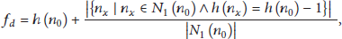
To compute $h (n_{x})$ , the synchronous identified interior nodes start to flood the WSN at roughly the same time as if they are a “root node”; then, each suspected boundary node records the minimal hop count to the root node, namely, the value of $h (n_{x})$ . During the network flooding, each suspected boundary node also records the minimal hop count from each of its 1-hop neighbor nodes to the root node, which are useful in the determination of $f_{d}$ by (1).

It is evident that the greater $f_{d}$ is, the further the corresponding suspected boundary node is away from actual interior nodes, and, on the contrary, the closer this node is to the boundaries of the WSN. In other words, $f_{d}$ differentiates a suspected boundary node from its 1-hop neighbor nodes in terms of the proximities to the boundaries of the WSN and is much helpful for finding boundary cycles in the next step.

To determine $f_{d}$ at each suspected boundary node, the message complexity is $O (n)$ because each node only needs to broadcast one message to its $1$ -hop neighbor nodes.

4.4. Searching for Boundary Cycles

In order to present our result in a meaningful way, we strive to obtain precise boundary cycles corresponding to both inner and outer boundaries of the WSN. To do so, the proposed algorithm searches all the suspected boundary nodes based on the same principle of the function $I N I T I A L I Z E (n_{0})$ and make the following two alterations.

First, unlike the function $I N I T I A L I Z E (n_{0})$ which only involves the nodes in $N_{2} (n_{0})$ and is realized in a centralized fashion, searching for boundary cycles deals with a relatively large number of suspected boundary nodes in the WSN and is thus suitable for a distributed implementation to avoid collecting the information of these suspected boundary nodes. To do so, each node with the locally minimal $f_{d}$ will serve as a starting node to launch a search process. To reduce the risk of having two search processes to conflict, a random waiting time is assigned to each starting node. However, if two searching processes unfortunately conflict, namely, one node is involved in both search processes, the one whose starting node's ID is smaller will stop, and, on the contrary, the other one will continue.

Second, node is arbitrarily expanded in the function $I N I T I A L I Z E (n_{0})$ but is expanded in a weighted way in the process of searching for boundary cycles. Specifically, the node with the maximal $f_{d}$ among all expandable nodes is preferentially expanded, which is the key factor for obtaining tight boundary cycles.

Like $L_{th}$ in the function $I N I T I A L I Z E (n_{0})$ , we need to define a similar parameter, denoted by $C_{th}$ , specifying the boundary cycle's length of the minimal boundary hole that can be recognized by the proposed algorithm. The choice of $C_{th}$ is dependent on physical environments as well as deployments of WSNs. But, if $C_{th}$ is set to a small number, the processes of searching for boundary cycles might be terminated early so as to fail to find boundary cycles, and, hence, $C_{th}$ is suggested to be greater than 10.

With boundary cycles, it is straightforward to distinguish an outer boundary from each inner boundary by comparing the lengths of their corresponding boundary cycles or by comparing the length of each boundary cycle with the perimeter of the WSN which can be roughly estimated based on the deployment information. Moreover, we can further refine the set of suspected boundary nodes by excluding the nodes which are more than 1-hop to boundary cycles.

Due to the possible conflicts caused by concurrent search processes, it is extremely difficult to analyze the message complexity of this step. In the ideal case that each suspected boundary node is expanded at most once, the number of messages is limited by the size of the suspected boundary node set and thus has the order of $O (n)$ .

To sum up, we can conclude that the message complexity of the proposed algorithm is $O (6 n)$ , which is comparable to the existing algorithms [20, 23, 30]. The message complexity of the algorithm in [20] is $O ((2 + a) n)$ , where a denotes the average number of seeds which every node falls into the scopes of and is certainly greater than 1. Seeds are usually selected in a random fashion, and, in order to guarantee that all nodes are in the scope of at least one seed, a relatively high number results, such that $2 + a$ can be as large as or even larger than $6$ . Moreover, explicit boundary cycles are unavailable by using this algorithm. The message complexity of the algorithm in [30] is $O (3 n)$ , and, likewise, explicit boundary cycles are unavailable. The message complexity of the algorithm in [23] is $O ((5 + b) n)$ , where b is greater than 1 and proportional to the number of inner holes. It is noticeable that if there is more than 1 hole in the network, the resulting message complexity can be larger than that of the proposed algorithm.

5. Practical Issues

In this section, we will discuss two practical issues in relation to applying the proposed algorithm.

5.1. Working with Realistic Channel Models

The algorithm is proposed in the idealized UDG model. Although the UDG model is simple, practical wireless communications can never satisfy it, and, hence, more realistic channel models, for example, the QUDG model, are developed. With the QUDG model, it is possible that the 2-hop isocontours of some actual boundary nodes can form closed cycles so as to satisfy the CLOSED-CYCLE condition, and, as a result, they are mistakenly identified as interior nodes (e.g., the boundary nodes with red circles in Figure 7(a)), which degrades the quality of the proposed algorithm.

Provided that an actual boundary node is identified as an interior node due to $f_{t} = 0$ , it can be observed that the majority of its 1-hop neighbor nodes are identified as suspected boundary nodes with $f_{t} = 1$ , but given an actual interior node with $f_{t} = 0$ , it is of small probability that the majority of its 1-hop neighbor nodes are identified as suspected boundary nodes. Then, it can be concluded that, for any identified interior node with $f_{t} = 0$ , if the ratio of the number of its 1-hop neighbor nodes with $f_{t} = 0$ to the total number of its 1-hop neighbor nodes is below a threshold $D_{th}$ , it is more likely to be an actual boundary node and its $f_{t}$ should be set to 1.

On these grounds, we design another heuristic operation, termed dilation, which to some extent is similar to the dilation operation in image processing, to adjust the value of $f_{t}$ . The dilation operation is performed between executing the function $I N I T I A L I Z E (n_{0})$ and the erosion operation. Besides the fact that some actual boundary nodes are changed from identified interior nodes to suspected boundary nodes by the dilation operation, some actual interior nodes might be changed to suspected boundary nodes as well, but such errors can be partly corrected by the following erosion operation.

If the dilation operation is performed, additional message transmission is required. Specifically, n messages are transmitted for the dilation, with the result that the total message complexity is increased by $O (n)$ .

5.2. Working with Low Node Densities

With decreasing the node density (e.g., by reducing the communication ranges), the number of 2-hop neighbor nodes of any node in a WSN is generally reduced, so that it becomes difficult to have the CLOSED-CYCLE condition satisfied, and, as a result, a portion of actual interior nodes are mistakenly grouped into the set of suspected boundary nodes, which remarkably damages the performance of the proposed algorithm. Therefore, we must alter our algorithm to be suitable for low-density WSNs.

One intuitive approach is including more neighbor nodes in the construction of the isocontour at each node. To do so, we can replace the original graph $G (V, E)$ in the execution of the function $I N I T I A L I Z E (n_{0})$ by its second power graph, denoted by $G^{2} (V^{2}, E^{2})$ . The 2-hop neighbor nodes of each node in the graph $G^{2} (V^{2}, E^{2})$ are actually the 3- and 4-hop neighbor nodes in the original graph $G (V, E)$ , and, hence, each node needs to collect all the neighbor nodes within 5 hops to accordingly construct the subgraph $G_{2} (V_{2}, E_{2})$ (see Pseudocode 1) of the power graph $G^{2} (V^{2}, E^{2})$ .

On replacing $g (V, E)$ by $G_{2} (V_{2}, E_{2})$ , it is equivalent that wireless communications follow a non-UDG model, with the result that some actual boundary nodes are identified as interior nodes, as considered under the QUDG model. Therefore, the dilation operation also is required here.

If power graphs are used in our algorithm, the messages transmitted are $5 n$ in the case of $G^{2} (V^{2}, E^{2})$ .

6. Performance Evaluation

We carry out extensive simulations in various scenarios, with the goal to evaluate the performance of the proposed algorithm with respect to the node density and distribution, the wireless channel model, existing boundary detection algorithms, and so forth.

6.1. Effect of Node Density

In this simulation, we assume the UDG model and deploy 2700 sensor nodes according to a uniform and random distribution in a square region of size 240 m with one circular hole of radius 50 m, which is the same as the WSN shown in Figure 2. The average node degree of the graph is varied by adjusting the communication radius of the UDG model. The choices of $C_{th}$ and $E_{th}$ are 15 and 0.7, respectively.

As illustrated in Figures 3 and 2(d), the proposed algorithm generates precise boundary cycles in general. Moreover, it can be observed that the larger the average node degree is, the more accurate the suspected boundary nodes are, the tighter the boundary cycles are, and, hence, the better the performance of the proposed algorithm is. The underlying reason is that a larger node density increases the possibility of forming a closed path enclosing each interior node due to having more 2-hop neighbor nodes and thus lowers the chance of mistakenly identifying interior nodes as suspected boundary nodes.

Figure 3

Results of applying the proposed algorithm in a WSN with a circular hole: (a) the average node degree is 15.6; (b) the average node degree is 22.4.

In the simulation, when the average node degree is below 14, the proposed algorithm cannot correctly recognize the boundaries due to insufficient connectivity. Faced with this situation, we use the second power graph instead of the original graph in the function of $I N I T I A L I Z E (n_{0})$ to improve the performance and add the heuristic dilation operation where $D_{th} = 0.2$ . As can be seen in Figure 4, the proposed algorithm is able to identify the boundaries even if the average node degree is as low as 9.2.

Figure 4

Using the power graph instead of the original graph to improve the performance of the proposed algorithm. The average node degree is 9.2.

Furthermore, we plot the results of applying the proposed algorithm in a couple of WSNs with interesting shapes in Figure 5.

Figure 5

Results of applying the proposed algorithm in two WSNs with interesting shapes. (a) The average node degree is 18.1; (b) the average node degree is 19.2.

6.2. Perturbed Grid Node Distribution

We still assume the UDG model but deploy 2700 sensor nodes on a grid of size 4 and perturb the position of each node by an independent and identically distributed random shift. The random shift is described by a pair of random variables with a uniform distribution in $[0,4]$ , representing x and y directions, respectively. In some circumstances, WSNs are deployed in an organized manner, say on a grid, but due to environmental influences, errors induced during deployment, or other factors, the actual position of each node often suffers a random shift from its specified position. Hence, this kind of distributions has a wide range of applications in WSNs, and this simulation is meaningful.

As illustrated in Figure 6, the proposed algorithm attains satisfactory results even if the average node degree is as low as 10 or 7 when using the power graph. Compared with the uniform and random node distribution, the perturbed grid node distribution has nodes deployed in a more symmetrical fashion, reduces the risk of having clusters and small holes, and consequently displays a superior performance.

Figure 6

Results for perturbed grid node distribution. (a) The average node degree is 7; (b) the average node degree is 10.

Figure 7

Results under the QUDG model. The average node degree is 16.5.

6.3. QUDG Model

In this simulation, we implement the proposed algorithm with the dilation operation under the QUDG model. Specifically, we use the same WSN as simulated in Figure 2 but assume that two nodes are connected if their distance is below 8 m and are disconnected if above 13. The choice of $D_{th}$ is 0.2.

As shown in Figure 7(b), the two actual boundary nodes surrounded by red circles, which are identified as interior nodes after the first step of our algorithm, are corrected to be suspected boundary nodes by the dilation operation and are finally included in the boundary cycles. Consequently, both the outer and inner boundaries are accurately detected.

6.4. Comparison with Other Methods

For comparison, we implement another three typical connectivity-based boundary detection algorithms [20, 23, 30]. In this simulation, we consider the same WSN that is simulated in Figure 2.

As can be seen in Figure 8, the algorithm in [20] can only identify a small portion of actual boundary nodes but cannot correctly find boundaries of the WSN; the algorithm in [30] can identify all the actual boundary nodes but mistakenly include many actual interior nodes. In contrast, the proposed algorithm obviously delivers superior results and appears to achieve nearly the same successful rate as the algorithm in [23], as shown in Figure 2.

Figure 8

Results of applying existing boundary detection algorithms. The average node degrees are 18.8. (a) The algorithm in [20]; (b) the algorithm in [30]; (c) the algorithm in [23].

7. Conclusions

In this paper, we developed an efficient, distributed, and connectivity-based boundary detection algorithm for WSNs. Our algorithm first identifies suspected boundary nodes by examining whether a closed path exists in the 2-hop isocontour of each node and encloses this node. Then, the erosion operation is applied to heuristically shrink the suspected boundary node set. At last, precise boundary cycles corresponding inner and outer boundaries are obtained and provide much valuable knowledge as to the boundaries of WSNs. In order to have the proposed algorithm work normally in low-density WSNs, we replaced the original graph of a WSN by its power graph in the first step of the algorithm. Moreover, we expanded our algorithm from the idealized UDG model to the more realistic QUDG model by introducing the dilation operation. In addition, a message complexity analysis confirmed the energy efficiency of our algorithm. Finally, we carried out a thorough evaluation verifying the accuracy of our algorithm and its applicability in both dense and sparse deployments of WSNs.

However, there are certain restrictions in applying the proposed algorithm. As shown in Figure 2(b), for each boundary, a certain “thickness” of nodes are discovered as suspected boundary nodes. When two boundaries are very close to each other, their relevant suspected boundary nodes are often connected, with the result that the proposed algorithm cannot separate them to correctly identify any of them. Empirically, any two boundaries should be at least 5 hops away from each other. Moreover, the proposed algorithm is not suitable for recognizing those holes with small perimeters.

In future work, we would like to discover more topology information (e.g., skeleton) of WSNs based on the proposed algorithm and to apply the proposed algorithm in more complicated scenarios, for example, 3-dimensional WSNs.

Footnotes

Conflict of Interests

The authors declare that there is no conflict of interests regarding the publication of this paper.

Acknowledgments

This work is supported by the Natural Science Foundation of Inner Mongolia under 2014MS0604, the Program of Higher-Level Talents of Inner Mongolia University under 125124, and the Inner Mongolia Autonomous Region Science and Technology Innovation Guide Reward Fund Project under 20121317.

References

Akyildiz

I. F.

Sankarasubramaniam

Cayirci

Wireless sensor networks: a survey

Computer Networks 2002 38 4 393 422

10.1016/S1389-1286(01)00302-4

2-s2.0-0037086890

Guo

Zhou

Jiang

Adaptive sensor placement and boundary estimation for monitoring mass objects

IEEE Transactions on Systems, Man, and Cybernetics B: Cybernetics 2008 38 1 222 232

10.1109/TSMCB.2007.910531

2-s2.0-39649085339

Ren

Zeng

Lou

Secure and fault-tolerant event boundary detection in wireless sensor networks

IEEE Transactions on Wireless Communications 2008 7 1 354 363

10.1109/TWC.2008.060550

2-s2.0-38349177828

Venkatesan

N. E.

Agarwal

Lalitha

Vijay Kumar

Distributed intrusion detection in the presence of correlated sensor readings: Signal-space and communication-complexity view-point

Ad Hoc Networks 2011 9 6 1015 1027

10.1016/j.adhoc.2010.07.015

2-s2.0-79955571614

Hoang

Lee

An efficient scheme for reducing overhead in data-centric storage sensor networks

IEEE Communications Letters 2009 13 12 989 991

10.1109/LCOMM.2009.12.091596

2-s2.0-73449092200

Liu

W.-J.

Feng

K.-T.

Three-dimensional greedy anti-void routing for wireless sensor networks

IEEE Transactions on Wireless Communications 2009 8 12 5796 5800

10.1109/TWC.2009.12.090220

2-s2.0-73049113409

Matrouk

Landfeldt

RETT-gen: A globally efficient routing protocol for wireless sensor networks by equalising sensor energy and avoiding energy holes

Ad Hoc Networks 2009 7 3 514 536

10.1016/j.adhoc.2008.07.002

2-s2.0-56749183853

Frey

Stojmenovic

On delivery guarantees and worst-case forwarding bounds of elementary face routing components in ad hoc and sensor networks

IEEE Transactions on Computers 2010 59 9 1224 1238

10.1109/TC.2010.107

MR2723704

2-s2.0-77955201883

Lee

Qiao

Demirbas

ABC: a simple geographic forwarding scheme capable of bypassing routing holes in sensor networks

Ad Hoc Networks 2010 8 4 361 377

10.1016/j.adhoc.2009.08.004

2-s2.0-75149141690

10.

Huang

Anderson

B. D. O.

Mao

Estimating distances via connectivity in wireless sensor networks

Wireless Communications and Mobile Computing 2014 14 5 541 556

10.1002/wcm.2204

2-s2.0-84856574506

11.

Jiang

Liu

Wang

Tian

Bai

Liu

Connectivity-based skeleton extraction in wireless sensor networks

IEEE Transactions on Parallel and Distributed Systems 2010 21 5 710 721

10.1109/TPDS.2009.109

2-s2.0-77950628125

12.

Liu

Jiang

Bai

Tan

Wang

Cai

Distance transform-based skeleton extraction and its applications in sensor networks

IEEE Transactions on Parallel and Distributed Systems 2013 24 9 1763 1772

10.1109/TPDS.2012.300

2-s2.0-84881061691

13.

Hung

K.-S.

Lui

K.-S.

On perimeter coverage in wireless sensor networks

IEEE Transactions on Wireless Communications 2010 9 7 2156 2164

10.1109/TWC.2010.07.080817

2-s2.0-77954739020

14.

Liu

On coverage of wireless sensor networks for rolling terrains

IEEE Transactions on Parallel and Distributed Systems 2012 23 1 118 125

10.1109/TPDS.2011.69

2-s2.0-82555186945

15.

Chen

Das

S. K.

Avoiding energy holes in wireless sensor networks with nonuniform node distribution

IEEE Transactions on Parallel and Distributed Systems 2008 19 5 710 720

10.1109/TPDS.2007.70770

2-s2.0-42549104040

16.

Fang

Gao

Guibas

L. J.

Locating and bypassing routing holes in sensor networks

Proceedings of the 23rd Annual Joint Conference of the IEEE Computer and Communications Societies (INFOCOM '04)

March 2004

Hong Kong, China

2458 2468

2-s2.0-8344224464

17.

Fekete

S. P.

Kröller

Pfisterer

Fischer

Buschmann

Neighborhood-based topology recognition in sensor networks

volume 3121

Proceedings of the 1st International Workshop on Algorithmic Aspects of Wireless Sensor Networks

July 2004

Turku, Finland

123 136

18.

Ghrist

Muhammad

Coverage and hole-detection in sensor networks via homology

Proceedings of the 4th International Symposium on Information Processing in Sensor Networks (IPSN ’05)

April 2005

Los Angeles, Calif, USA

254 260

10.1109/IPSN.2005.1440933

2-s2.0-33744946538

19.

Fekete

S. P.

Kaufmann

Kröller

Lehmann

A new approach for boundary recognition in geometric sensor networks

Proceedings of the 17th Canadian Conference on Computational Geometry

August 2005

Windsor, Canada

82 85

20.

Funke

Klein

Hole detection or: “how much geometry hides in connectivity?”

Proceedings of the 22nd ACM Symposium on Computational Geometry

2006

Sedona, Ariz, USA

377 385

21.

Dong

Neighborhood-based distributed topological hole detection algorithm in sensor networks

Proceedings of the IET International Conference on Wireless, Mobile and Multimedia Networks

November 2006

Hangzhou, China

1 4

22.

Kröller

Fekete

S. P.

Pfisterer

Fischer

Deterministic boundary recognition and topology extraction for large sensor networks

Proceedings of the 17th ACM-SIAM Symposium on Discrete Algorithms

Miami, Fla, USA

ACM

1000 1009

10.1145/1109557.1109668

MR2373827

23.

Wang

Gao

Mitchell

J. S. B.

Boundary recognition in sensor networks by topological methods

Proceedings of the 12th Annual International Conference on Mobile Computing and Networking (MOBICOM '06)

September 2006

Los Angeles, Calif, USA

122 133

2-s2.0-33751047930

24.

Sahoo

P. K.

Hsieh

Sheu

J.-P.

Boundary node selection and target detection in wireless sensor network

Proceedings of the 4th IEEE and IFIP International Conference on Wireless and Optical Communications Networks (WOCN '07)

July 2007

Singapore

1 5

10.1109/WOCN.2007.4284126

2-s2.0-50449091249

25.

Saukh

Sauter

Gauger

Marrón

P. J.

Rothermel

On boundary recognition without location information in wireless sensor networks

Proceedings of the International Conference on Information Processing in Sensor Networks (IPSN '08)

April 2008

St. Louis, Mo, USA

207 218

10.1109/IPSN.2008.11

2-s2.0-51249107627

26.

Khan

Mokhtar

Merabti

A new self-detection scheme for sensor network boundary recognition

Proceedings of the 34th IEEE Conference on Local Computer Networks (LCN '09)

October 2009

Zurich, Switzerland

241 244

10.1109/LCN.2009.5355078

2-s2.0-77951268279

27.

Fayed

Mouftah

H. T.

Localised alpha-shape computations for boundary recognition in sensor networks

Ad Hoc Networks 2009 7 6 1259 1269

10.1016/j.adhoc.2008.12.001

2-s2.0-64049100948

28.

Chen

Liang

Shen

Coordinate-free distributed algorithm for boundary detection in wireless sensor networks

Proceedings of the 54th Annual IEEE Global Telecommunications Conference (GLOBECOM '11)

December 2011

Houston, Tex, USA

1 5

10.1109/GLOCOM.2011.6134264

2-s2.0-84863166630

29.

Chen

Y.-H.

Chung

W.-H.

G.-K.

Zhang

Kuo

S.-Y.

Optimal self boundary recognition with two-hop information for ad hoc networks

Proceedings of the IEEE Wireless Communications and Networking Conference (WCNC '12)

April 2012

Paris, France

1910 1914

10.1109/WCNC.2012.6214099

2-s2.0-84864339300

30.

Chu

W.-C.

Ssu

K.-F.

Decentralized boundary detection without location information in wireless sensor networks

Proceedings of the IEEE Wireless Communications and Networking Conference (WCNC '12)

April 2012

Paris, France

1720 1724

10.1109/WCNC.2012.6214061

2-s2.0-84864359655

31.

Zhou

Jin

A robust boundary detection algorithm based on connectivity only for 3D wireless sensor networks

Proceedings of the 31st Annual Joint Conference of the IEEE Computer and Communications Societies (INFOCOM '12)

March 2012

1602 1610

10.1109/INFCOM.2012.6195529

2-s2.0-84861645098

32.

Zhang

Tay

W. P.

K. H.

Gaiti

Distributed boundary estimation for spectrum sensing in cognitive radio networks

Proceedings of the IEEE Wireless Communications and Networking Conference (WCNC '13)

April 2013

4107 4112

10.1109/WCNC.2013.6555235

2-s2.0-84881566522

33.

Kim

Kwak

Kim

H. J.

Joint detection and tracking of boundaries using cooperative mobile sensor networks

Proceedings of the IEEE International Conference on Robotics and Automation (ICRA '13)

May 2013

Karlsruhe, Germany

889 894

34.

Shu

Song

Fisher information of mine collapse hole detection based on sensor nodes connectivity

International Journal of Distributed Sensor Networks 2013 2013 7

306496

10.1155/2013/306496

35.

Chen

Level set based co verage holes detection and holes healing scheme in hybrid sensor network

International Journal of Distributed Sensor Networks 2013 2013 9

297383

10.1155/2013/297383

36.

Ganeriwal

Kumar

Srivastava

M. B.

Timing-sync protocol for sensor networks

Proceedings of the 1st international conference on Embedded networked sensor systems (SenSys '03)

November 2003

Los Angeles, Calif, USA

138 149

2-s2.0-11244272924

37.

Sichitiu

M. L.

Veerarittiphan

Simple, accurate time synchronization for wireless sensor networks

Proceedings of the IEEE Wireless Communications and Networking Conference (WCNC '03)

March 2003

New Orlenas, La, USA

1266 1273

Recognizing Boundaries in Wireless Sensor Networks Based on Local Connectivity Information

Abstract

1. Introduction

2. Related Work

3. Problem Formulation

4. Proposed Boundary Detection Algorithm

4.1. Initializing f t

Pseudocode 1: The pseudo code of the function I n i t i a l i z e ( n 0 ) . P u s h ( e x p a n d i n g _ p a t h , n r ) pushes n r into the stack e x p a n d i n g _ p a t h and P o p ( e x p a n d i n g _ p a t h ) pops the top node from the stack e x p a n d i n g _ p a t h .

4.2. Performing the Erosion Operation

4.3. Determining f d

4.4. Searching for Boundary Cycles

5. Practical Issues

5.1. Working with Realistic Channel Models

5.2. Working with Low Node Densities

6. Performance Evaluation

6.1. Effect of Node Density

6.2. Perturbed Grid Node Distribution

6.3. QUDG Model

6.4. Comparison with Other Methods

7. Conclusions

Footnotes

Conflict of Interests

Acknowledgments

References

4.1. Initializing $f_{t}$

Pseudocode 1: The pseudo code of the function $I n i t i a l i z e (n_{0})$ . $P u s h (e x p a n d i n g_p a t h, n_{r})$ pushes $n_{r}$ into the stack $e x p a n d i n g_p a t h$ and $P o p (e x p a n d i n g_p a t h)$ pops the top node from the stack $e x p a n d i n g_p a t h$ .

4.3. Determining $f_{d}$