Sage Journals: Discover world-class research

Abstract

We improve the typical GM car-following model. In order to describe the impacts of the lateral offset between the vehicles in car-following state, this paper proposes time distance to measure the drivers' attention of driving environment and uses generalized expectation headway to describe the ideal driving state of the driver. Take the difference between the actual and expected headway as the important standard for driver to decide whether to speed up or slow down. Then take the drivers' attentions and the expected headway as the decision-making factors, and consider them while revising the GM car-following model. The numerical simulation shows the improved GM model conforms to the general driving behavior, enhances the function of the typical model, and strengthens the model stability.

1. Introduction

Car-following model was used to describe the driving behavior of following vehicle facing the actions of the leading vehicle in the single lane with limit of overtaking. It played an important role in the traffic theory and was widely used in the field of microscopic traffic simulation, smart driving, traffic safety, and so forth. The researches of car-following have been lasting for years and made a series of results [1 –3], and the General Motor car-following model was proposed firstly and considered the most typical model in those research results.

The GM car-following is jointly proposed by Gazis et al. [4]. This model regarded the difference between the leading and following car as the source of stimulation and combined with the space headway and velocity to obtain the driver's acceleration decision making. A variety of car models are derived by the GM modeling idea [5 –10]. Lee proposed a GM model with memory effect; the basic idea was that the driver reacts based on the stimulation of a period of time rather than the point-in-time. Herman established a model to describe the impact on driver form the multivehicle in the front; it considered the driver received the effect not only from the single leading car but the continuous traffic flow before.

GM model is sensitive to the changing of the leading vehicle and has the advantages of high accuracy in the microsimulation. However the structure of the model is flawed. In GM model, the relative velocity, as the stimuli, was placed in the model structure as multiplier terms. It results in the fact that the following car would not adjust its speed regardless of the space when the leading and following car have the same velocity. It is clearly inconsistent with the actual situation.

A fundamental assumption of the traditional car-following model is that all vehicles are travelling in the center of the lane [11 –16]. But it is difficult to achieve this ideal state. Gunay studied the transverse distribution of the vehicle in the lane [6]; it showed the vehicle occurrence frequency decreasing from the center to sides in the lane, similar to normal distribution, and exhibited the lateral offset phenomenon was prevalent. Meanwhile, the traditional car-following model only considered the effect from the leading vehicle but ignored the front vehicle in the adjacent lane, and this would case a certain extent impact on the driver.

This paper proposes improved GM car-following model. It presents the expectation time headway into the traditional GM model as stimulation except the speed difference between the leading and the following vehicle to enhance the stability of the model. Add the lateral offset and the lateral vehicle effect factors into the model to expand its scope of application.

2. Materials and Methods

2.1. Generalized Expectation Headway

In traditional model, the expectation headway is the headway the following driver hopes to maintain with the leading vehicle in travelling. In this case, there is no lateral offset between the two vehicles. This paper expands the range of the application of the expectation headway from car-following in one-dimensional straight line to the two-dimensional flat space and proposes the generalized expectation headway; it is shown in Figure 1.

Figure 1:

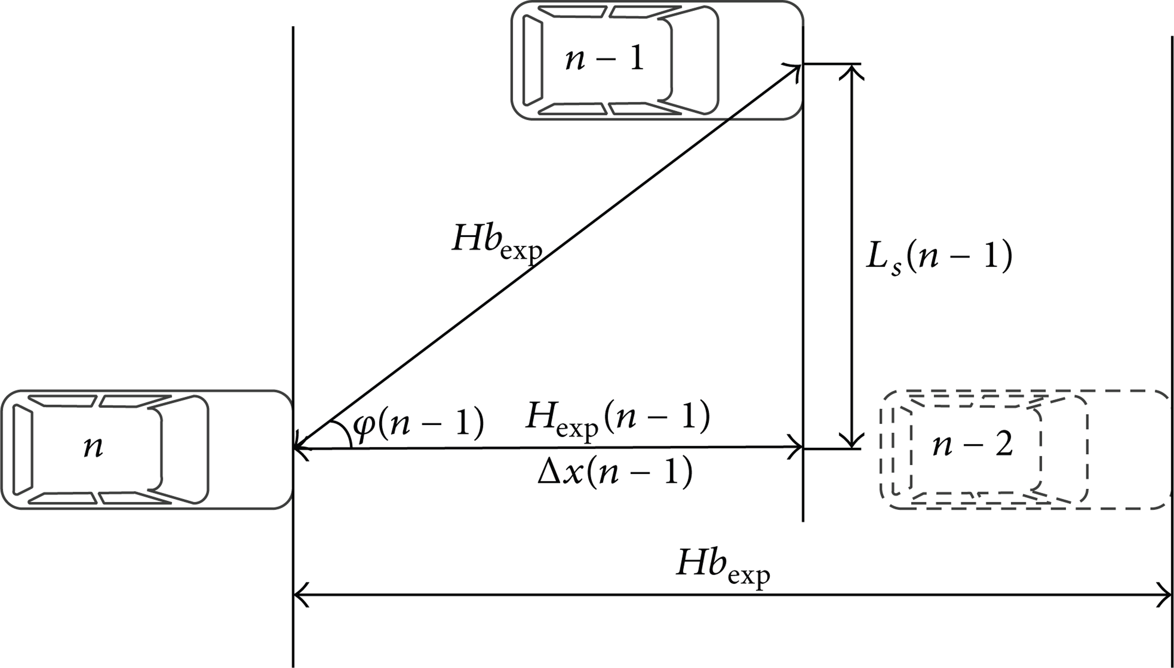
Diagram of generalized expectation headway.

The Hb_{exp ⁡} in Figure 1 is the expectation headway of the traditional car model, named basic headway. It shows the headway the driver hopes to keep with the leading car and is usually a fixed value. In Figure 1, the generalized expectation headway of the driver in vehicle numbered n to vehicle n − 2 is basic headway. As the lateral vehicle n − 1, the generalized expectation headway of vehicle n is the projective value's function of the basic headway Hb_{exp ⁡}. It is positive correlation with the Hb_{exp ⁡}(n − 1), named H_{exp ⁡}. H_{exp ⁡} is also associated with the lateral offset L_s(n − 1) of the vehicle n − 1. With the L_s(n − 1) increasing, the angle ϕ(n − 1) formed from the vehicle n and n − 1 in Figure 1 would be growing, in case the projection of Hb_{exp ⁡}(n − 1) in the vehicle n driving direction weakens. And make the H_{exp ⁡}(n − 1) reduce. In addition, if the laterally offset L_s(n − 1) is fixed, with the decreasing of the distance Δx(n − 1) in the direction along the vehicle driving, the angle ϕ(n − 1) will be growing and causing the H_{exp ⁡}(n − 1) weakened.

The generalized expectation headway has effects in the car-following state. Except the angle ϕ(n − 1), the H_{exp ⁡}(n − 1) in Figure 1 is also associated with the allowed maximum lateral offset in car-following; denote it by L_{s_thr}. Obviously, the vehicles n and n − 1 are in the car-following state if the L_s(n − 1) is not bigger than L_{s_thr}; otherwise, n − 1 and n are in the different lanes; the generalized expectation headway is not fit.

The smaller the difference between the L_s(n − 1) and L_{s_thr} is, the smaller the H_{exp ⁡}(n − 1) is. The generalized expectation headway is performed by the following model:

H_{\exp} (n - 1) = λ_{3} (L_{s} (n - 1)) \cdot \sqrt{\frac{Δ x^{2} (n - 1)}{L_{s}^{2} (n - 1) + Δ x^{2} (n - 1)}} \cdot H b_{\exp} .

(1)

The λ₃ is sensitivity coefficient inversely related to the L_s; formula (2) shows its forms:

λ_{3} (L_{s} (n - 1)) = 1 - \frac{L_{s} (n - 1)}{L_{s_thr}} (L_{s} (n - 1) < L_{s_thr}) .

(2)

Obviously, when L_s(n − 1) ≤ L_{s_thr}, λ₃ belongs to the area [0, 1], and it decreases monotonically with L_s(n − 1) increasing. If L_s(n − 1) > L_{s_thr}, the generalized expectation headway has no effect; the value of λ₃ will not affect the acceleration the GM model output.

2.2. The Driver's Space Attention

The driver's degree of concern of his front space could be considered to be represented as time distance. In the one-dimensional linear space, the time distance is the required time that the vehicle needs to reach the special position. In two-dimensional area, the driver's degree of concern is changing with the spatial position varying. If the speed is under certain preconditions, the closer to the driver's front angle, the higher the degree of driver's concern. In the case of the same angle, the distances determine the strength of the degree of driver's concern. Therefore, formula (3) performs the driver's space attention:

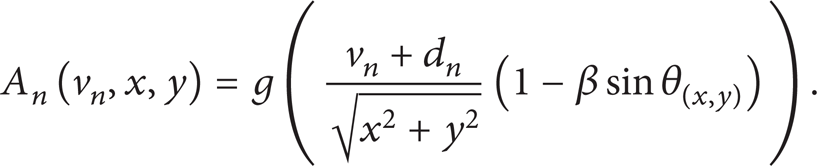
A_{n} (v_{n}, x, y) = g (\frac{v_{n} + d_{n}}{\sqrt{x^{2} + y^{2}}} (1 - β \sin θ_{(x, y)})) .

(3)

The A_n(v_n, x, y) is the space attention of vehicle n's driver about the space point (x, y) under the current velocity v_n. (x, y) is the position coordinate, and g() is a monotonically increasing function. β is undetermined coefficients; sinθ_{(x, y)} is the sine value between the vehicle n driving direction and the connection line between vehicle and point (x, y). d_n marks the vehicle running state is acceleration or deceleration; when the vehicle has been in the accelerated state, under the same conditions the driver's attention will be strengthened and weakened to a certain extent in the deceleration state.

2.3. The Improved GM Car-Following Model Establishing

The traditional GM car-following model is shown in the following formulation:

a_{n} (t + T) = \frac{λ v_{n}^{m} (t + T)}{{[x_{n - 1} (t) - x_{n} (t)]}^{l}} [v_{n - 1} (t) - v_{n} (t)] .

(4)

a(t + T) is the acceleration of vehicle n at time point t + T. v_{n − 1}(t) and v_n(t) are the velocity of vehicles n − 1 and n at the time t. x_{n − 1}(t) and x_n(t) are the locations of the vehicles n − 1 and n at time t. T is reaction time of the driver. λ is a sensitivity coefficient. m and l are parameters to be determined.

Formula (4) can be rewritten as the following formula:

a_{n} (t + T) = λ {(\frac{v_{n} (t) + a_{n} (t) T}{x_{n - 1} (t) - x_{n} (t)})}^{m} \frac{[v_{n - 1} (t) - v_{n} (t)]}{{[x_{n - 1} (t) - x_{n} (t)]}^{m - l}} .

(5)

The ${((v_{n} (t) + a_{n} (t) T) / (x_{n - 1} (t) - x_{n} (t)))}^{m}$ is the basis form of the driver's space attention function, and convert it in the form of formula (3), and the application of the model extends to the two-dimensional area. And synchronization adds the gap between the expected and actual headway to the model; finally the improved GM car-following is shown by the following formula:

a_{n} (t + T) = λ_{1} {[\frac{v_{n} (t) + a_{n} (t) T}{Δ x} (1 - β \frac{L_{s}}{Δ x})]}^{m} \times [\frac{Δ v}{Δ x^{l - m}} + rec (Δ v, Δ v_{thr}) rec (L_{s}, L_{s_thr}) λ_{2} (\frac{1}{H_{\exp}} - \frac{v_{n}}{Δ x})] .

(6)

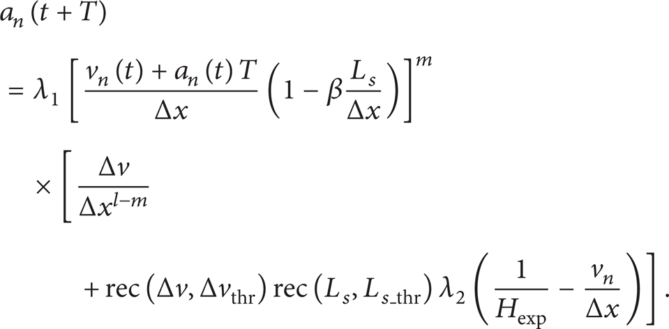
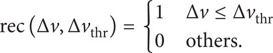
Δx = x_{n − 1}(t) − x_n(t), Δv_n = v_{n − 1}(t) − v_n(t), and rec() is shown as formula (7). The excepted headway is mainly for solving the defects of the traditional GM car-following model, that when the leading and following vehicles have the similar speed, the output of the model is zero. Therefore, the excepted headway does not occur when the speed difference is large:

rec (Δ v, Δ v_{thr}) = \{\begin{cases} 1 & Δ v \leq Δ v_{thr} \\ 0 & others . \end{cases}

(7)

3. Results and Discussion

Make the numerical simulation analysis of the improved GM car-following model.

3.1. The Characteristics of Space Headway

The state stability of the space headway in car-following is an important criterion in evaluating model for the leading and following vehicle. Use the numerical simulate method to achieve the car-following process and focus on analyzing the space headway varying characteristics when the leading and following vehicle have the same initial speed (i.e., the speed difference is zero). Some typical situation is proposed, as specified in Table 1.

Table 1:

The set of the vehicle initial parameter analyzing the space headway.

Simulation number	The initial speed of the leading vehicle (vehicle n − 1) (m/s)	Speed of following vehicle (vehicle n) (m/s)	The initial space headway (m)	Speed changing of vehicle n − 1 m/s (10⁻¹ s)

1	20	20	80	20(0), 15(100)
2	20	20	60	20(0), 15(100)
3	20	20	40	20(0), 15(100)

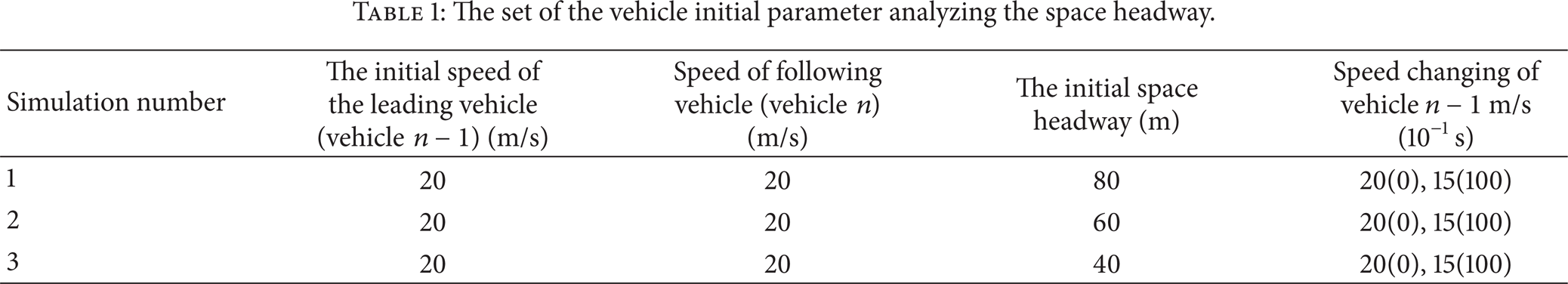
In Table 1, v₁(t₁), v₂(t₂), ⋯, v_m(t_m) in the column labeled the “speed changing of Vehicle n − 1” means the speed of vehicle n − 1 is v_i at time t_i, and keep a constant rate of changing the speed to v_{i + 1} at time t_{i + 1}. Finally, maintain a speed v_m after the time t_m. t₁ ~ t_m means the moment point, and the v₁ ~ v_m correspond to the vehicle velocity for different points in time.

Make the numerical simulation apply the improved and original GM car-following model; set the simulation time interval 0.1 seconds. The parameters select the typical parameters values and take m = 1, l = 2, λ = λ₁ = 10, λ₂ = 5, H_{exp ⁡} = 3. The simulation result is shown in Figure 2.

Figure 2:

The space headway changing comparing between the improved and typical GM car-following model.

It can be seen from Figure 2(a), the following vehicle (n) will slow down to maintain a safe headway when the initial space headway is small, then pay attention to the leading vehicle (n − 1) running state changing. So the space headway first increases and then decreases. And under the big initial headway (simulation numbers 2 and 3), the following vehicle's space headway gradually reduces and the variation are relatively flat. Finally, the following vehicle is able to stabilize at a fixed value in the above cases.

Figure 2(b) shows the simulation results of typical GM car-following model. It can be found that the original GM model overreliance on speed difference between the leading and following vehicle decide to accelerate or decelerate. Even the space headway is small, it still reduces. Once the initial conditions are more demanding, it may cause the vehicle's rear end. In simulation numbers 2 and 3, the space headway changing are similar to the simulation 1 in Figure 2(b). But if the leading and following vehicles have the same speed, the following driver would stop adjusting the velocity. This makes the space headway much larger than the corresponding to the situation in Figure 2(a).

Compare Figures 2(a) and 2(b); when the leading vehicle motion state changing and parameter settings are in consistent case, the original GM model ultimately produces completely different simulation results due to the different initial conditions, and the improved GM car-following solves this problem.

3.2. Propagation Character of Speed

After the model is applied to the individual vehicle in the queue, if the first vehicle changes its velocity, this variation of the propagation characteristics is an important criterion in evaluating model. If the changing of speed in the dissemination process is expanded, it indicates that the model is unstable. And if this rate of changing in the communication process gradually decayed, it indicates that the model is stable.

Analyze the speed spreading situation of the vehicles queue with the numerical simulation, as shown in Table 2.

Table 2:

The set of the vehicle initial parameter in analyzing the velocity spreading.

Simulation number	The initial speed of the first vehicle in queue (m/s)	Speed of other vehicles in queue (m/s)	The initial space headway (m)	Speed changing of vehicle 1 m/s (10⁻¹ s)

4	20	20	60	20(0), 22.5(50), 17.5(150), 20(200)
5	20	20	40	20(0), 22.5(50), 17.5(150), 20(200)
6	20	25	60	20(0), 22.5(50), 17.5(150), 20(200)
7	20	25	80	20(0), 22.5(50), 17.5(150), 20(200)

The meaning of the columns in Table 2 is similar to Table 1, and the vehicles in queue are numbered from 1 to 30 from the first to end, a total of 30 vehicles. The model parameters setting is the same as in Figure 2.

Simulate the situation 4~7 in the table. The changing of the vehicles speed is shown in Figure 3. Because of the space limitation, there only are the first five vehicles speed shown in Figure 3.

Figure 3:

Changing of the vehicles' velocity in the queue.

In Figure 3(a), because the initial headway is the expected headway, the queue is in a steady state. The rear vehicles adjust the speed with the vehicle 1 velocity changing. This adjusting has a certain lag and reflects the role of reaction time.

In Figure 3(b), for the small headway at the initial moment, drivers attempt to protect safety to slow down; even the first vehicle has been in an accelerated state. Until reaching a safe headway, the vehicle starts to follow the vehicle 1 state to adjust the speed.

In Figure 3(c), the rear vehicles initial speeds are higher than the first; for security purposes, the initial stage, the rear vehicles will decelerate till reduce to a certain extent and then follow with vehicle 1. In Figure 3(d), remaining rear vehicles have high initial velocity, but decreases weaken because of the large initial space headway.

In summary, under the improved GM car-following model constraint, no matter what initial state, the rear vehicles in the queue will tend to the first vehicle motion state adjusting the velocity. And the variation would be attenuated with position in queue backward and be impacted by the reaction time, the speed transmission with a certain lag.

3.3. Microsimulation

Execute numerical simulation of the typical and improved GM car-following, and compare with the measured data to verify the model effect. The acceleration is the output of the car-following model and also the quantification of the speed changing degree. So the velocity could describe the real-time vehicle running state and avoid tiny gap of acceleration causing large relative error around zero. Therefore, this paper uses the output speed as the standard to evaluate the consistency degree of the vehicle running state.

The measured data are from the US Federal Highway Administration website. The data collected in a north-south direction of the main road Lankershim in Los Angeles, California, United States. The data collection session is 8:30 to 9:00, the traffic state back to the flat peak just from the morning rush hour. Traffic density is moderate with the car-following behavior common and strong representation. Select 10 groups' car-following behavior data to analyze with the numerical simulation. The relevant parameters are set as the value in Figure 2 except the expected headway H_{exp ⁡}. Because of driving behavior feature on the urban road, set the expected headway H_{exp ⁡}. The simulation results are shown in Table 3.

Table 3:

Error of velocity between the typical and improved GM car-following model.

Number	Amount of data	Relative error of the mode output and the measured data
Number	Amount of data	Typical GM car-following model	Improved GM car-following model

1	237	13.3%	12.0%
2	296	15.8%	8.1%
3	160	12.3%	11.7%
4	151	8.2%	6.2%
5	224	16.0%	15.3%
6	81	6.3%	5.2%
7	212	14.9%	14.8%
8	268	13.8%	11.8%
9	251	6.9%	6.6%
10	84	25.2%	16.3%

When the speed difference of the following and leading car is large, the output of the improved GM car-following model is similar to the typical GM model. But if the speed difference is small, the improved GM model plays important role. So when the car-following vehicles are in the relatively stable state, the improved GM car-following model has improved the output accuracy.

3.4. The Lateral Offset Effect in Car-Following State

Apply the model this paper established to each vehicle in a continuous vehicle flow. Number the vehicles in queue 1 to n from front to back. The vehicle running states changing set is shown in Table 4.

Table 4:

The set of the vehicle initial parameters in analyzing the lateral impact.

Simulation number	The initial speed of the first vehicle in queue (m/s)	Speed of other vehicles in queue (m/s)	The initial space headway (m)	The lateral position changing of the first vehicle in queue (m (10⁻¹ s))

8	10	10	30	0(0), 2(100), 2(700), 0(900)
9	15	15	30	0(0), 0(100), 2(300), 2(700), 0(900)
10	15	15	60	0(0), 0(100), 2(200), 0(300)
11	15	15	40	0(0), 0(100), 2(200), 0(300)

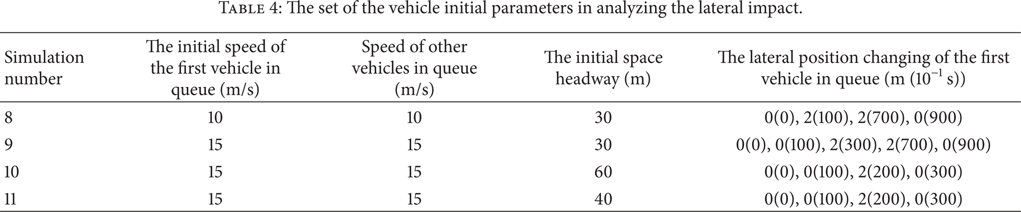
In Table 4, l₁(t₁), l₂(t₂), ⋯, l_m(t_m) in the column labeled the “lateral position changing of the first vehicle in queue” means the first vehicle is deviated from the lane centerline at time t_i, and keep a constant rate of changing the lateral position deviated from the lane centerline l_{i + 1} at time t_{i + 1}. Finally, maintain a lateral offset l_m after the time t_m. t₁ ~ t_m mean the moment point, and the l₁ ~ l_m correspond to the vehicle lateral offset for different points in time.

The simulation numbers 8~11 in Table 4 are, respectively, different initial state simulation. The lateral positions of the first vehicle in queue changing and other vehicles in the queue running states are shown in Figure 4. Figure 4 listed the space headway changing of the top five cars in the vehicle queue. Set the generalized expectation headway 3 s.

Figure 4:

Changing of the space headway.

In Figure 4(a), the space headway of the second vehicle in the queue decreases with the velocity growing and is smaller than other following vehicles when the lateral offset of first vehicle gradually increases and reaches a steady value. At the time the first vehicle's lateral offset begins to decrease and eventually restore zero value, the space headway of the second vehicle also restores the initial state. The space headway of other vehicles in the queue changed with the second vehicle state varying, and the degree of this change gradually decays as the vehicle's position backward. Thus, the first vehicle lateral offset impacts on the rear following vehicle obviously. The queue running state would be affected, but the impact is relatively limited.

Figure 4(b) corresponds to the simulation number 9 in Table 4. In the initial state the vehicles in queue have relatively smaller space headway. Except the first, other vehicles slow down to increase the headway with the first vehicle's speed unchanged. This situation in Figure 4(b) is the increasing of the space headway. The space headway of the second vehicle significant decrease compared with other vehicles while the first vehicle lateral offset growing (10~30 seconds), and increases when the laterally offset of first vehicle reduced.

Figure 4(c) corresponds to the simulation number 10 in Table 4. In the initial stage the vehicles in queue own the relatively big headway. Except the first, other ones accelerate to reduce the headway, and the space headway reduces obviously in this process (0~10 s). The lateral offset of the first vehicle has fluctuation in the 10~20 s stage, and it impacts on the second car obviously. The space headway of the second vehicle continues to decrease, and the magnitude of change is much larger than other ones. Until the first vehicle gradually get back to the lane centerline, the space headway of second vehicle becomes stable.

For the simulation number 11 shown in Figure 4(d). The space headway of the vehicle in queue except the first one increases, but the lateral offset of the first vehicle interrupts the process of the second vehicle, so that the space headway of vehicle 2 is reduced. Until the lateral offset vehicle 1 gets back to zero, vehicle 2 space headway would grow and finally equal to other vehicles.

In summary, the lateral offset of the leading vehicle impacts on the following driver. It is embodied in the same state, the more the lateral offset is, the smaller the space headway between the two vehicles is when the state restores stability. And if the state of vehicles changes, laterally offset fluctuations will affect the normal variety of the space headway and even change its changing direction.

3.5. The Lateral Offset Effect in No-Car-Following State

As Figure 5 shows, the adjacent front and back vehicles are in the adjacent lane. If the vehicle n is faster than vehicle n − 1 in Figure 5, within a certain time, vehicle n will inevitably overtake the vehicle n − 1. And in this overtaking process, vehicle n will inevitably be affected by n − 1.

Figure 5:

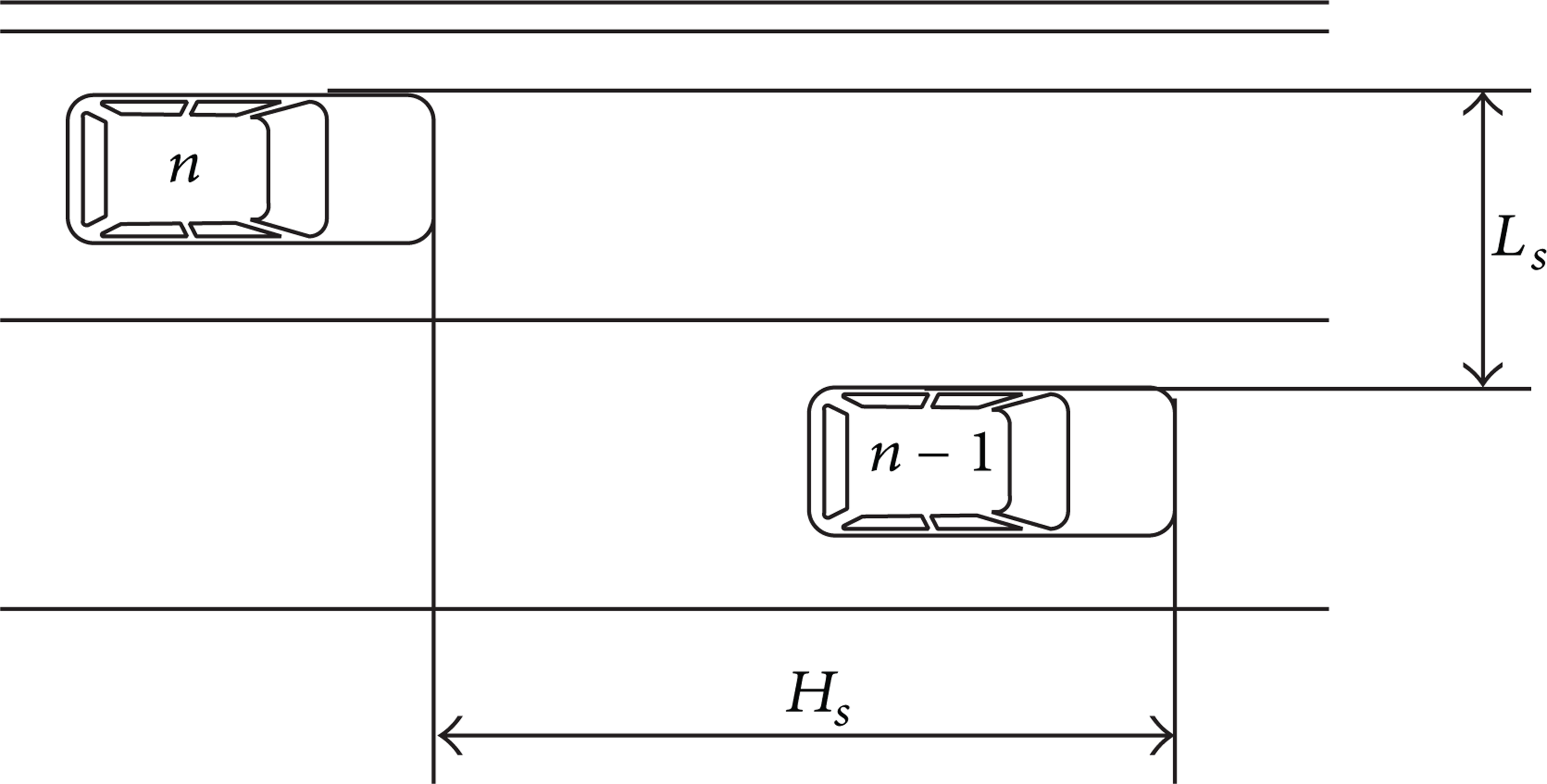
The impact of the vehicles in adjacent lane.

The initial settings of numerical simulation are shown in Table 5. Assume that the n − 1 maintained a steady speed and the lateral position in the overtaking processing of vehicle n. And lateral offset does not occur during the vehicle n running. Then assume the vehicle attempt to achieve the desired speed with a constant acceleration. The longitudinal spacing in Table 5 refers to the distance along the road directions between the vehicles n and n − 1, that is, the H_s in Figure 5. The lateral spacing distance refers to the vertical direction of the road between the two vehicles, that is, the L_s in Figure 5.

Table 5:

Initial settings of numerical simulation.

Simulation number	Initial velocity of vehicle n − 1	Initial velocity of vehicle n	Desired velocity of vehicle n	Vehicles n − 1 and n
Simulation number	Initial velocity of vehicle n − 1	Initial velocity of vehicle n	Desired velocity of vehicle n	Initial longitudinal spacing	Initial lateral spacing

12	0	10	25	100	3.5
13	5	20	25	100	3.5

Figure 6 is the vehicles' running situation of simulation and corresponds to the different settings in Table 5. In simulation number 12, vehicle n − 1 is held stationary. The vehicle n gradually approaches and finally overtake the vehicle n − 1. And in the processing of closing, as the distance decreasing, the speed of vehicle n will have a certain magnitude of decrease. After overtaking, the vehicle is in a free state; the speed keeps increasing until it reaches the desired value. The processing is shown in Figures 6(a) and 6(b).

Figure 6:

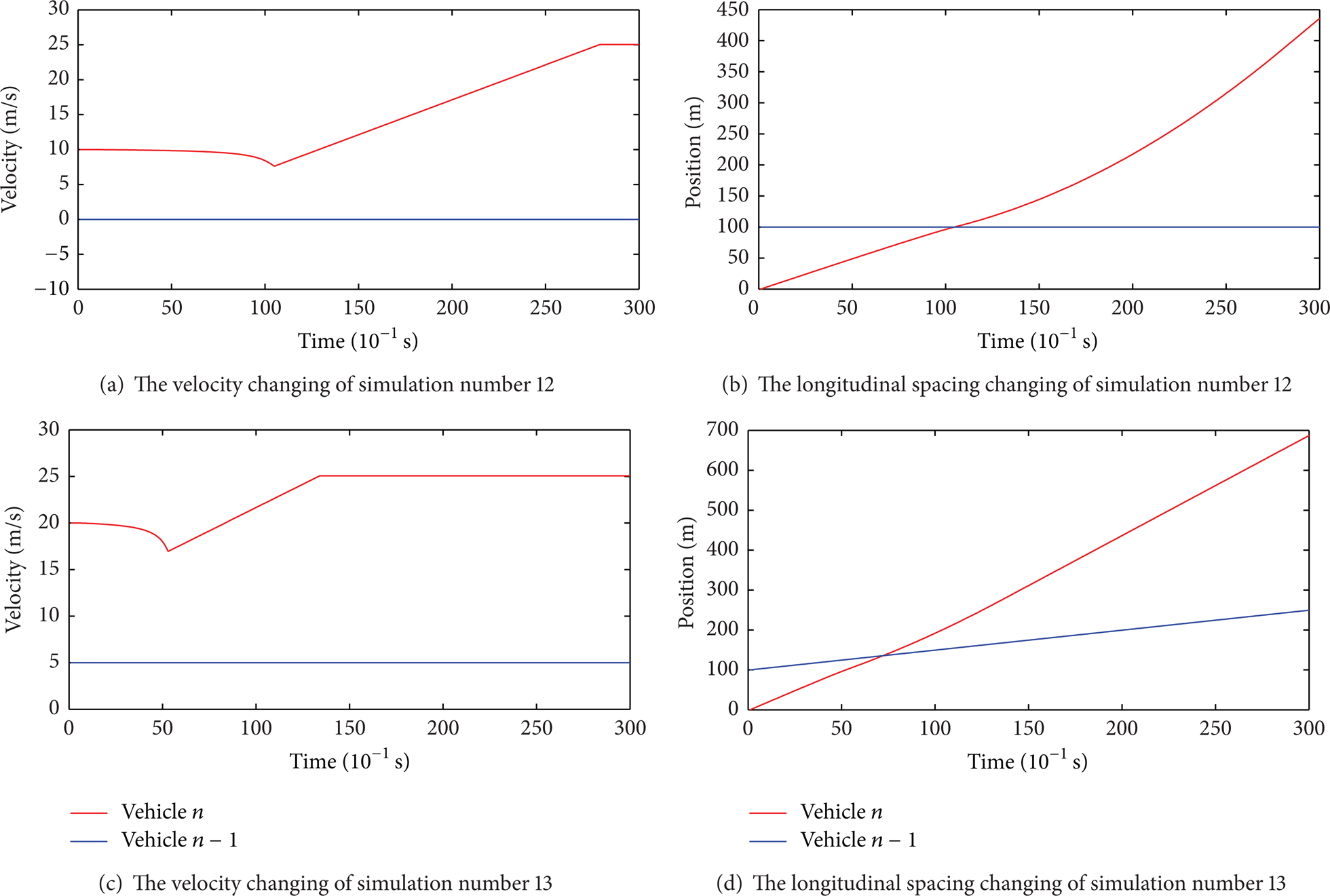
The running state of vehicles under lateral influence.

In simulation number 13, the vehicle n − 1 maintains a certain speed. With closing to the n − 1, the velocity of vehicle n will gradually decrease, and the amplitude increases with distance decreasing. Until the completion of the overtaking, the velocity of vehicle n gradually recovers and eventually reaches the desired speed.

In summary, as Figure 6 shows, vehicle n is impacted by the front vehicle in adjacent lane and causes the deceleration. This is consistent with the actual situation. In actual driving, it happens mainly due to psychological care of driver to prevent the adjacent vehicles sudden changing lane. In the improved GM model, reflect this driving behavior and formation of this state of mind from the simulation results.

4. Conclusion

This paper proposes the improved GM car-following model. By generalized expectation headway, this model solves the problem of the typical GM car-following model that the output results are zeros when the leading and following vehicle have the same velocity whatever values of other parameters are. And the model is improved to be able to make a quantitative description of driver attention to the two-dimensional area. The numerical simulation shows that the model complies with the general rules of the actual driving, and the stability has a more substantial enhancement.

Conflict of Interests

The authors declare that there is no conflict of interests regarding the publication of this paper.

Footnotes

Acknowledgments

This work is supported by the National Science Foundation of China (nos. 51278220, 51278454, and 51108208) and China Postdoctoral Science Foundation (20141M551178).

References

Brackstone

and McDonald

, “Car-following: a historical review,” Transportation Research Part F, vol. 2, no. 4, pp. 181–196, 1999.

Kesting

and Treiber

, “Calibrating car-following models by using trajectory data methodological study,” Transportation Research Record, vol. 2088, pp. 148–156, 2008.

Hollander

and Liu

, “The principles of calibrating traffic microsimulation models,” Transportation, vol. 35, no. 3, pp. 347–362, 2008.

Gazis

D. C.

Herman

, and Rothery

R.W.

, “Nonlinear follow-the- leader models of traffic flow,” Operations Research, vol. 9, pp. 545–567, 1961.

Jin

Wang

D.-H.

, and Huang

Z.-Y.

, “Staggered car-following induced by lateral separation effects in traffic flow,” Physics Letters A, vol. 376, no. 3, pp. 153–157, 2012.

Gunay

, “Car following theory with lateral discomfort,” Transportation Research Part B, vol. 41, no. 7, pp. 722–735, 2007.

Jin

Wang

Tao

, and Li

, “Non-lane-based full velocity difference car following model,” Physica A, vol. 389, no. 21, pp. 4654–4662, 2010.

Zhu

H. B.

and Dai

S. Q.

, “Analysis of car-following model considering driver's physical delay in sensing headway,” Physica A: Statistical Mechanics and Its Applications, vol. 387, no. 13, pp. 3290–3298, 2008.

Ossen

and Hoogendoorn

S. P.

, “Heterogeneity in car-following behavior: theory and empirics,” Transportation Research C: Emerging Technologies, vol. 19, no. 2, pp. 182–195, 2011.

10.

Jin

, and Wang

, “Assessment of expressway traffic safety using gaussian mixture model based on time to collision,” International Journal of Computational Intelligence Systems, vol. 4, no. 6, pp. 1122–1130, 2011.

11.

Jin

Huang

Z.-Y.

Tao

P.-F.

, and Wang

D.-H.

, “Car-following theory of steady-state traffic flow using time-to-collision,” Journal of Zhejiang University: Science A, vol. 12, no. 8, pp. 645–654, 2011.

12.

Wagner

, “Analyzing fluctuations in car-following,” Transportation Research Part B: Methodological, vol. 46, no. 10, pp. 1384–1392, 2012.

13.

Gunawan

F. E.

, “Two-vehicle dynamics of the car-following models on realistic driving condition,” Journal of Transportation Systems Engineering and Information Technology, vol. 12, no. 2, pp. 67–75, 2012.

14.

Zheng

Suzuki

, and Fujita

, “A car-following model based on discrete choice theory,” Journal of Transportation Systems Engineering and Information Technology, vol. 12, no. 5, pp. 31–38, 2012.

15.

Wang

Bengler

, and Wets

, “Discrete dynamics in transportation system,” Discrete Dynamics in Nature and Society, vol. 2013, Article ID 234970, 2 pages, 2013.

16.

Guo

Wang

Guo

, and Zhao

, “Modeling lane-keeping behavior of bicyclists using survival analysis approach,” Discrete Dynamics in Nature and Society, vol. 2013, Article ID 197518, 6 pages, 2013.

An Improved General Motor Car-Following Model considering the Lateral Impact

Abstract

1. Introduction

2. Materials and Methods

2.1. Generalized Expectation Headway

2.2. The Driver's Space Attention

2.3. The Improved GM Car-Following Model Establishing

3. Results and Discussion

3.1. The Characteristics of Space Headway

3.2. Propagation Character of Speed

3.3. Microsimulation

3.4. The Lateral Offset Effect in Car-Following State

3.5. The Lateral Offset Effect in No-Car-Following State

4. Conclusion

Conflict of Interests

Footnotes

Acknowledgments

References