Numerical Investigation for the Modeling of the Magnetic Buoyancy Force during the Natural Convection of Air in a Square Enclosure

Abstract

Numerical computations are carried out for natural convection of air in a two-dimensional square enclosure under a nonuniform magnetic field and together with the gravity field. The nonuniform magnetic field is supplied by a cubic permanent magnet placed above the enclosure. Two kinds of the expressions for the magnetizing force are considered and compared in the numerical computations. The flow and temperature fields, the magnetizing force field and the Nusselt number for two kinds of magnetizing force expressions are all presented in this paper. The numerical results reveal that the natural convection inside the enclosure does not depend on the types of the expressions for magnetizing force.

1. Introduction

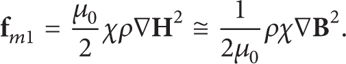
Recent development of superconducting materials at high temperature has enabled us to utilize commercial superconducting magnets that produce the magnetic flux density up to 10 Tesla or so. By using such strong magnets, various new findings have been reported for the last decades [1–5]. In the fields of fluid mechanics and heat transfer, the application of such high magnetic field on the control of natural convection heat transfer has received considerable attention. Some of the examples can be found in a series of papers reported by Ozoe's group [6–13]. The control of natural convection heat transfer is based on the principle that the magnetizing force acts at a molecular level depending on the values of magnetic susceptibility of fluid. Therefore, the utilization of the magnetizing force is equivalent to the local gravity control within the region where the high gradient magnetic field exists. In a single phase with isothermal state, both the magnetizing force and gravitational force are the conservative force and hence convection does not occur by them no matter how strong they are. In order to rise the convection, both the magnetic field gradient and the temperature gradient are necessary. In a normal expression, the magnetizing force is written by the equation as follows [14]:

${\mathbf{f}}_{m\mathrm{1}}=\frac{{\mu }_{\mathrm{0}}}{\mathrm{2}}\chi \rho \nabla {\mathbf{{\rm H}}}^{\mathrm{2}}\cong \frac{\mathrm{1}}{\mathrm{2}{\mu }_{\mathrm{0}}}\rho \chi \nabla {\mathbf{B}}^{\mathrm{2}}.$

(1)

On the other hand, the magnetizing force can be expressed in another way as follows [15]:

${\mathbf{f}}_{m\mathrm{2}}=-\frac{{\mu }_{\mathrm{0}}{\mathbf{H}}^{\mathrm{2}}}{\mathrm{2}}\nabla \left(\rho \chi \right)\cong -\frac{{\mathbf{B}}^{\mathrm{2}}}{\mathrm{2}{\mu }_{\mathrm{0}}}\nabla \left(\rho \chi \right).$

(2)

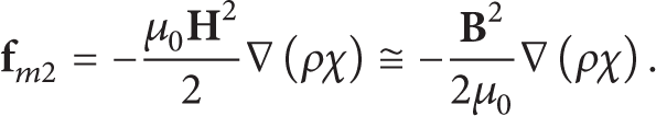
These two kinds of formulas confuse us. Most of the previous studies about the magnetothermal convection use (1) for the calculation of magnetizing force. There has been little study on the magnetothermal convection using (2) for the calculation of magnetizing force.

In this paper, we focus on the comparison of these expressions for magnetizing force for the natural convection flow and also on the possibility of heat transfer control of natural convection of air by using a permanent magnet (neodymium-iron-boron) which does not need any power supply from outside like a superconducting magnet.

2. Physical Model

The physical model considered in this paper is shown in Figure 1. Two kinds of two-dimensional square enclosures are considered. Figure 1(a) shows the physical model-I in which the left wall is heated and right wall is cooled isothermally, and the other two walls are thermally insulated. Figure 1(b) shows the physical model-II in which the bottom wall is heated and top wall is cooled isothermally, and the other two walls are thermally insulated. Physical model-I is a physically stable model for natural convection, but physical model-II is a physically unstable model as priorly studied in [16]. We employ physical model-II as a comparison with physical model-I.

Figure 1:

Configuration of simulation models: (a) PM-I and (b) PM-II.

A cubic permanent magnet with the residual magnetic flux density in the z direction is put on the top of the square enclosure. The length of both the magnet and square enclosure is L = 0.05 m. There is a gap of 1 mm between the magnet and the square enclosure.

3. Mathematical Equations

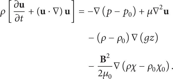
In this paper, the magnetizing force obtained by (1) is named force type I (FT-I) and the magnetizing force obtained by (2) is named force type II (FT-II). In the following, we consider the derivation of the magnetic buoyancy force for FT-II since we can easily find the derivation of the magnetic buoyancy force for FT-I in the references, for instance, in [7]. The Navier-Stokes equation including the magnetizing force FT-II is as follows:

$\rho \left[\frac{\partial \mathbf{u}}{\partial t}+\left(\mathbf{u}·\nabla \right)\mathbf{u}\right]=-\nabla p+\mu {\nabla }^{\mathrm{2}}\mathbf{u}-\rho \nabla \left(gz\right)-\frac{{\mathbf{B}}^{\mathrm{2}}}{\mathrm{2}{\mu }_{\mathrm{0}}}\nabla \left(\rho \chi \right).$

(3)

We assume that the air is an incompressible Newtonian fluid and the Boussinesq approximation is employed. When we consider the isothermal state, the fluid density and susceptibility would be constant, and convection does not arise even in both the gravity and magnetic fields. Hence we get

$\mathbf{0}=-\nabla p_{\mathrm{0}}-{\rho }_{\mathrm{0}}\nabla \left(gz\right)-\frac{{\mathbf{B}}^{\mathrm{2}}}{\mathrm{2}{\mu }_{\mathrm{0}}}\nabla \left({\rho }_{\mathrm{0}}{\chi }_{\mathrm{0}}\right).$

(4)

The properties with the subscript 0 denote the value at a reference temperature, while those without the subscript denote the variables depending on the local temperature within the computational domain. Taking the difference between (3) and (4) yields

$\rho \left[\frac{\partial \mathbf{u}}{\partial t}+\left(\mathbf{u}·\nabla \right)\mathbf{u}\right]=-\nabla \left(p-p_{\mathrm{0}}\right)+\mu {\nabla }^{\mathrm{2}}\mathbf{u}-\left(\rho -{\rho }_{\mathrm{0}}\right)\nabla \left(gz\right)-\frac{{\mathbf{B}}^{\mathrm{2}}}{\mathrm{2}{\mu }_{\mathrm{0}}}\nabla \left(\rho \chi -{\rho }_{\mathrm{0}}{\chi }_{\mathrm{0}}\right).$

(5)

The density can be expressed by a Taylor expansion (keeping two terms only) around a reference state θ₀ as follows:

$\rho ={\rho }_{\mathrm{0}}+{\left(\frac{\partial \rho }{\partial \theta }\right)}_{\mathrm{0}}\left(\theta -{\theta }_{\mathrm{0}}\right)+\cdots .$

(6)

On the other hand, the thermal volume coefficient of expansion β is defined for fluid as follows [17]:

$\beta =\frac{1}{V}{\left(\frac{\partial V}{\partial \theta }\right)}_p=\frac{1}{1/\rho }{\left(\frac{\partial \left(1/\rho \right)}{\partial \theta }\right)}_p=-\frac{1}{\rho }{\left(\frac{\partial \rho }{\partial \theta }\right)}_p.$

(7)

Then, (6) can be written as follows:

$\rho -{\rho }_{\mathrm{0}}={\left(\frac{\partial \rho }{\partial \theta }\right)}_{\mathrm{0}}\left(\theta -{\theta }_{\mathrm{0}}\right)=-{\rho }_{\mathrm{0}}{\beta }_{\mathrm{0}}\left(\theta -{\theta }_{\mathrm{0}}\right).$

(8)

The volume expansion coefficient for an ideal gas becomes as follows:

$\begin{array}{c}\beta =-\frac{\mathrm{1}}{\rho }\frac{\partial \rho }{\partial \theta }=-\frac{\mathrm{1}}{\rho }\frac{\partial }{\partial \theta }\left(\frac{p}{R\theta }\right)=-\frac{\mathrm{1}}{\rho }\frac{p}{R}\frac{\partial }{\partial \theta }\left(\frac{\mathrm{1}}{\theta }\right)\\ \hspace{1em}=-\frac{\mathrm{1}}{\rho }\frac{p}{R}\left(-\frac{\mathrm{1}}{{\theta }^{\mathrm{2}}}\right)=\frac{p}{\rho R{\theta }^{\mathrm{2}}}=\frac{\mathrm{1}}{\theta }.\hfill \end{array}$

(9)

The difference of ρχ can be written as

$\rho \chi -{\left(\rho \chi \right)}_{\mathrm{0}}={\left(\frac{\partial \rho \chi }{\partial \theta }\right)}_{\mathrm{0}}\left(\theta -{\theta }_{\mathrm{0}}\right)={\left(\chi \frac{\partial \rho }{\partial \theta }+\rho \frac{\partial \chi }{\partial \theta }\right)}_{\mathrm{0}}\left(\theta -{\theta }_{\mathrm{0}}\right).$

(10)

Magnetic susceptibility of air is a function of temperature, where C is a constant [14]. Consider

$\frac{\partial \chi }{\partial \theta }=\frac{\partial }{\partial \theta }\left(\frac{C}{\theta }\right)=-\frac{\chi }{\theta }.$

(11)

Then, (9) can be written as follows:

$\rho \chi -{\left(\rho \chi \right)}_{\mathrm{0}}={\left(-\chi \frac{\rho }{\theta }-\rho \frac{\chi }{\theta }\right)}_{\mathrm{0}}\left(\theta -{\theta }_{\mathrm{0}}\right)=-\mathrm{2}{\rho }_{\mathrm{0}}{\beta }_{\mathrm{0}}{\chi }_{\mathrm{0}}\left(\theta -{\theta }_{\mathrm{0}}\right).$

(12)

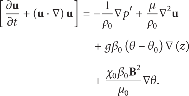
Given p = p₀ + p′, we get the momentum equation from (5) as follows:

$\left[\frac{\partial \mathbf{u}}{\partial t}+\left(\mathbf{u}·\nabla \right)\mathbf{u}\right]=-\frac{\mathrm{1}}{{\rho }_{\mathrm{0}}}\nabla p^{\prime }+\frac{\mu }{{\rho }_{\mathrm{0}}}{\nabla }^{\mathrm{2}}\mathbf{u}+g{\beta }_{\mathrm{0}}\left(\theta -{\theta }_{\mathrm{0}}\right)\nabla \left(z\right)+\frac{{\beta }_{\mathrm{0}}{\chi }_{\mathrm{0}}{\mathbf{B}}^{\mathrm{2}}}{{\mu }_{\mathrm{0}}}\nabla \theta .$

(13)

Thus, the government equations for the natural convection caused by the magnetic buoyancy force for FT-II are summarized as follows.

• Continuity equation is as follows:

  $\nabla ·\mathbf{u}=\mathrm{0}.$

  (14)

• Momentum equation is as follows:

  $\left[\frac{\partial \mathbf{u}}{\partial t}+\left(\mathbf{u}·\nabla \right)\mathbf{u}\right]=-\frac{\mathrm{1}}{{\rho }_{\mathrm{0}}}\nabla p^{\prime }+\frac{\mu }{{\rho }_{\mathrm{0}}}{\nabla }^{\mathrm{2}}\mathbf{u}+g{\beta }_{\mathrm{0}}\left(\theta -{\theta }_{\mathrm{0}}\right)\nabla \left(z\right)+\frac{{\chi }_{\mathrm{0}}{\beta }_{\mathrm{0}}{\mathbf{B}}^{\mathrm{2}}}{{\mu }_{\mathrm{0}}}\nabla \theta .$

  (15)

• Energy equation is as follows:

  $\rho c_p\left[\frac{\partial \theta }{\partial t}+\left(\mathbf{u}·\nabla \right)\theta \right]=\lambda {\nabla }^{\mathrm{2}}\theta .$

  (16)

The momentum equation for the magnetic buoyancy force FT-I is expressed as follows:

$\left[\frac{\partial \mathbf{u}}{\partial t}+\left(\mathbf{u}·\nabla \right)\mathbf{u}\right]=-\frac{\mathrm{1}}{{\rho }_{\mathrm{0}}}\nabla p^{\prime }+\frac{\mu }{{\rho }_{\mathrm{0}}}{\nabla }^{\mathrm{2}}\mathbf{u}+g{\beta }_{\mathrm{0}}\left(\theta -{\theta }_{\mathrm{0}}\right)\nabla \left(z\right)-\frac{{\chi }_{\mathrm{0}}{\beta }_{\mathrm{0}}\left(\theta -{\theta }_{\mathrm{0}}\right)}{{\mu }_{\mathrm{0}}}\nabla {\mathbf{B}}^{\mathrm{2}}.$

(17)

In all the subsequent computation, the reference temperature θ₀ is arbitrarily selected to be equal to the temperature of the cold wall; that is ${\theta }_0=\theta {}_c$ .

The initial condition (t < 0) is

• u = w = 0, θ₀ = θ _c .

Boundary conditions for physical model PM-I are

• on the wall: u = w = 0;

• left wall: θ = θ _h ;

• right wall: θ = θ _c ;

• top and bottom walls: ∂θ/∂z = 0.

Boundary conditions for physical model PM-II are

• on the wall: u = w = 0;

• bottom wall: θ = θ _h ;

• top wall: θ = θ _c ;

• left and right walls: ∂θ/∂x = 0.

The local Nusselt number represents the ratio of heat transfer rate by convection to that by conduction in the fluid. Nu_local is given by

${\text{Nu}}_{\text{local}}=\frac{h_{\text{local}}L}{\lambda }.$

(18)

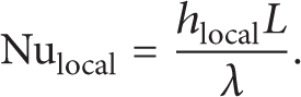
The local heat transfer coefficient h_local is defined as

$h_{\text{local}}=\frac{\lambda }{{\theta }_h-{\theta }_c}\left|\frac{\partial \theta }{\partial n}\right|.$

(19)

4. Calculation of Magnetic Field and Numerical Method

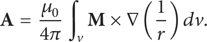
In this study, the magnetic field is assumed to be provided by a cubic permanent neodymium-iron-boron (Nd-Fe-B) magnet which has a high-energy product and could drive the gas-free convection easily under a gradient temperature field. The magnetic field is solved using the vector potential method [18]. The magnetic induction B can be expressed as the curl of the vector potential A:

$\mathbf{B}=\nabla \times \mathbf{A}\mathbf{.}$

(20)

The magnetic vector potential generated by the permanent magnet at the calculated point is as follows:

$\mathbf{A}=\frac{{\mu }_{\mathrm{0}}}{\mathrm{4}\pi }{{\displaystyle \int }}_v\frac{\mathbf{M}\times {\mathbf{r}}_{\mathrm{1}}}{r^{\mathrm{2}}}dv,$

(21)

where v is the volume of the magnet, r is the distance from the element volume dv of the magnet to the point where the field is calculated, and r ₁ is the unit vector along r. When the calculated field point is fixed and the source point, that is, the center of element volume dv, is moving, the gradient of 1/r is

$\nabla \left(\frac{\mathrm{1}}{r}\right)=\frac{{\mathbf{r}}_{\mathrm{1}}}{r^{\mathrm{2}}}.$

(22)

Equation (21) can be rewritten as

$\mathbf{A}=\frac{{\mu }_{\mathrm{0}}}{\mathrm{4}\pi }{{\displaystyle \int }}_v\mathbf{M}\times \nabla \left(\frac{\mathrm{1}}{r}\right)dv.$

(23)

According to the curl calculus identities,

$\begin{array}{c}\mathbf{M}\times \nabla \left(\frac{\mathrm{1}}{r}\right)=-\nabla \times \left(\frac{\mathbf{M}}{r}\right)+\frac{\mathrm{1}}{r}\left(\nabla \times \mathbf{M}\right),\\ {{\displaystyle \int }}_v\left(\nabla \times \frac{\mathbf{M}}{r}\right)dv=-{{\displaystyle \int }}_S\frac{\mathbf{M}}{r}\times \mathbf{d}\mathbf{a}\mathbf{,}\end{array}$

(24)

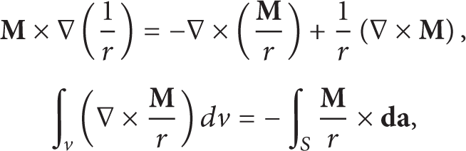
where S is the surface bounding the volume v and da is the element of area in the direction normal to the surface S.

Then, the magnetic vector potential can be rewritten as

$\mathbf{A}=\frac{{\mu }_{\mathrm{0}}}{\mathrm{4}\pi }{{\displaystyle \int }}_S\frac{\mathbf{M}\times \mathbf{n}}{r}da+\frac{{\mu }_{\mathrm{0}}}{\mathrm{4}\pi }{{\displaystyle \int }}_v\frac{\nabla \times \mathbf{M}}{r}dv.$

(25)

Here, M × n represents an equivalent surface current density; the curl of M represents an equivalent volume current density. Since the magnetic vector potential can be ascribed to the distributions of surface current density and volume current density, we can write down the value of B using the Biot-Savart law [18]:

$\mathbf{B}=\frac{{\mu }_{\mathrm{0}}}{\mathrm{4}\pi }{{\displaystyle \int }}_S\frac{\mathbf{M}\times \mathbf{n}\times {\mathbf{r}}_{\mathrm{1}}}{r^{\mathrm{2}}}da+\frac{{\mu }_{\mathrm{0}}}{\mathrm{4}\pi }{{\displaystyle \int }}_v\frac{\nabla \times \mathbf{M}\times {\mathbf{r}}_{\mathrm{1}}}{r^{\mathrm{2}}}dv.$

(26)

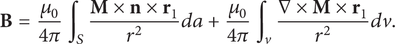
Thus, if we know the permanent magnet's magnetization M, we can find the equivalent current densities. Then, we can use the equivalent currents to calculate B by the upper equation.

The computed magnetic induction along the central axis perpendicular to the pole surface is compared with the distribution equation [19] of a cubic magnet. Figure 2 shows the comparison of distribution of z-component of magnetic induction along the central axis perpendicular to the pole surface of a cubic magnet with those reported by Yamakawa et al. [19]. The result is nearly the same. Just near the magnet there has been a maximum error less than 4%.

Figure 2:

Comparison of distribution of magnetic flux density along central axis of cubic magnet.

In this study, the permanent magnet is applied on the top of the upper wall, and the poles of the magnet are lined parallel to the z-direction. The square enclosure is placed under the cubic magnet in the middle of the y-side (normal to x-z plane in Figure 1) and parallel to the x-z plane. The computed magnetic field and the magnetic lines produced by the cubic permanent magnet in the simulation domain are shown in Figure 3.

Figure 3:

Magnetic field and magnetic lines in the simulation domain.

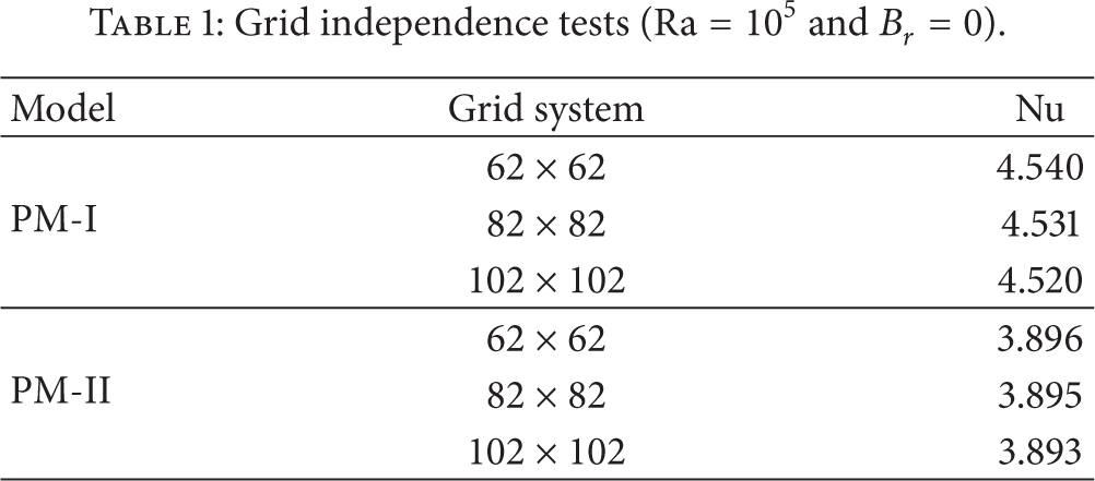
The SIMPLE algorithm developed by Patankar [20] is used to solve the coupled heat transfer and fluid flow problem. The power-law scheme is used in the finite difference formulation of convection terms and a fine grid system is selected to raise the simulation precision. The grid-independence test for the solutions is carried out with three grid systems. The averaged Nusselt numbers at different grid systems are presented in Table 1. Since the difference between three grid systems is less than 0.5% for both physical models studied in this paper, the grid system 82 × 82 is selected for all computations. The physical properties of air and other constants used are summarized in Table 2.

Table 1:

Grid independence tests (Ra = 10⁵ and B _r = 0).

Model	Grid system	Nu
PM-I	62 × 62	4.540
	82 × 82	4.531
	102 × 102	4.520
PM-II	62 × 62	3.896
	82 × 82	3.895
	102 × 102	3.893

Table 2:

Parameters and constants used in report (300 K, 1 atm).

Acceleration coefficient of gravity (g)	9.8 m/s2
Prandtl number (Pr)	0.702
Density of gas at 300 K (ρ)	1.177 kg/m3
Kinematic viscosity of gas (ν)	15.718 × 10−6 m2/s
Viscosity of gas (μ)	18.5 × 10−6 Pa·s
Thermal conductivity (λ)	2.646 × 10−2 W/(m·K)
Thermal diffusivity of gas (α)	22.45 × 10−6 m2/s
Mass magnetic susceptibility of oxygen (χ)	1.738 × 10−6 m3/kg
Cold wall temperature (θ c )	300.0 K
Volumetric coefficient of expansion of gas (β)	1/300.0 (1/K)
Magnetic permeability of free space	4π × 10−7 H/m

5. Results and Discussion

All the computations are carried out at Ra = 10⁵ with three different residual flux densities of permanent magnet. Two physical models under gravity field and magnetic field are studied for two types of magnetizing force expressions. The model with gravity field only is also studied for comparison.

5.1. Comparison of Magnetizing Force Fields

Figure 4 shows the magnetizing force fields with two types of magnetizing forces (FT-I and FT-II) for a physical model PM-I. From these figures we can find that the magnetizing forces are quite different from the gravitational force (B _r = 0) and there are quite different magnetizing force vectors for different types of magnetizing force. The magnetizing force has an adverse direction with the gravitational force. The magnetizing force increased with increase in the strength of the magnetic fields. For physical model PM-I with force type FT-I, there is larger magnetizing force near the top and hot wall of the enclosure and it decreases from the hot wall to the cold wall and from top wall to the bottom wall. This can be seen clearly in a large magnetic field, such as B _r = 2.5 T. But for force type FT-II, the magnetic fields are quite different. There is larger magnetizing force near the top and cold wall and the force decreases from the cold wall to the hot wall, which is quite different from the distribution of the magnetizing force of PM-I with FT-I. By comparing Figure 4(a) with Figure 4(b) we can clearly see that the value of the magnetizing force of FT-I is larger than that of magnetizing force FT-II.

Figure 4:

Magnetizing force vectors of physical model PM-I with two types of magnetizing forces: (a) PM-I with FT-I and (b) PM-I with FT-II.

Figure 5 shows the magnetizing force fields with two types of magnetizing forces (FT-I and FT-II) for a physical model PM-II. The gravity field is quite different from that of PM-I and the magnetizing force is also quite different. The magnetizing force increases with increases of magnetic field strength. There have been symmetric magnetizing force fields for both types of the magnetizing forces. The value of magnetizing force FT-II is larger than that of FT-I, which is quite different from that of PM-I.

Figure 5:

Magnetizing force vectors of physical model PM-II with two types of magnetizing forces: (a) PM-II with FT-I and (b) PM-II with FT-II.

5.2. Comparison of Velocity Fields

Figure 6 shows the velocity vectors with two types of magnetizing forces for physical model PM-I. When there is gravity only, B _r = 0, there is one vortex with two cores in the center and the vortex rotates clockwise in the enclosure. When magnetic field is added to the gravity field, the natural convection decreases due to the effect of the magnetic field which has an adverse direction comparing to the gravitational field. When the magnetic strength is 2.5 T, a new vortex with counterrotating direction formed in the region near the top and cold walls. The strength of the vortex in the center of the enclosure decreases and the new vortex will be larger and stronger with the increase in the strength of magnetic field. Although the distribution of the magnetizing forces is quite different for different force types of physical model PM-I, the distributions of the velocity field are quite similar. We hardly find the difference between the velocity fields for PM-I with FT-I and FT-II.

Figure 6:

Velocity vectors of physical model PM-I with two types of magnetizing forces: (a) PM-I with FT-I and (b) PM-I with FT-II.

For physical model-II with two types of magnetizing forces, a vortex formed in the enclosure with a clockwise direction when there is gravity field only, shown in Figure 7. When the magnetic strength is weak, B _r = 0.5 T, as the magnetizing force is very weak compared with the gravitational force as shown in Figure 5, the velocity fields are much more similar to the velocity field with gravity only. When the magnetic field B _r is 1.5 T and 2.5 T, there are two symmetric vortices with counterrotating directions in the enclosure and the vortices are similar to each other for force types FT-I and FT-II. When B _r = 0.5 T, it is interesting that the rotating direction is adverse for force types I and II. The reason may be that the magnetic field has very weak effect on the natural convection in the enclosure when the magnetic field is very weak, and the natural convection under gravity field is unstable for physical model PM-II. This result is in reasonable agreement with the prior study of Ozoe and Churchill [16]. From Figures 6 and 7 we can find that the velocity field with magnetizing force type FT-I is consistent with the field with magnetizing force type FT-II for both physical models although the magnetizing force fields are quite different.

Figure 7:

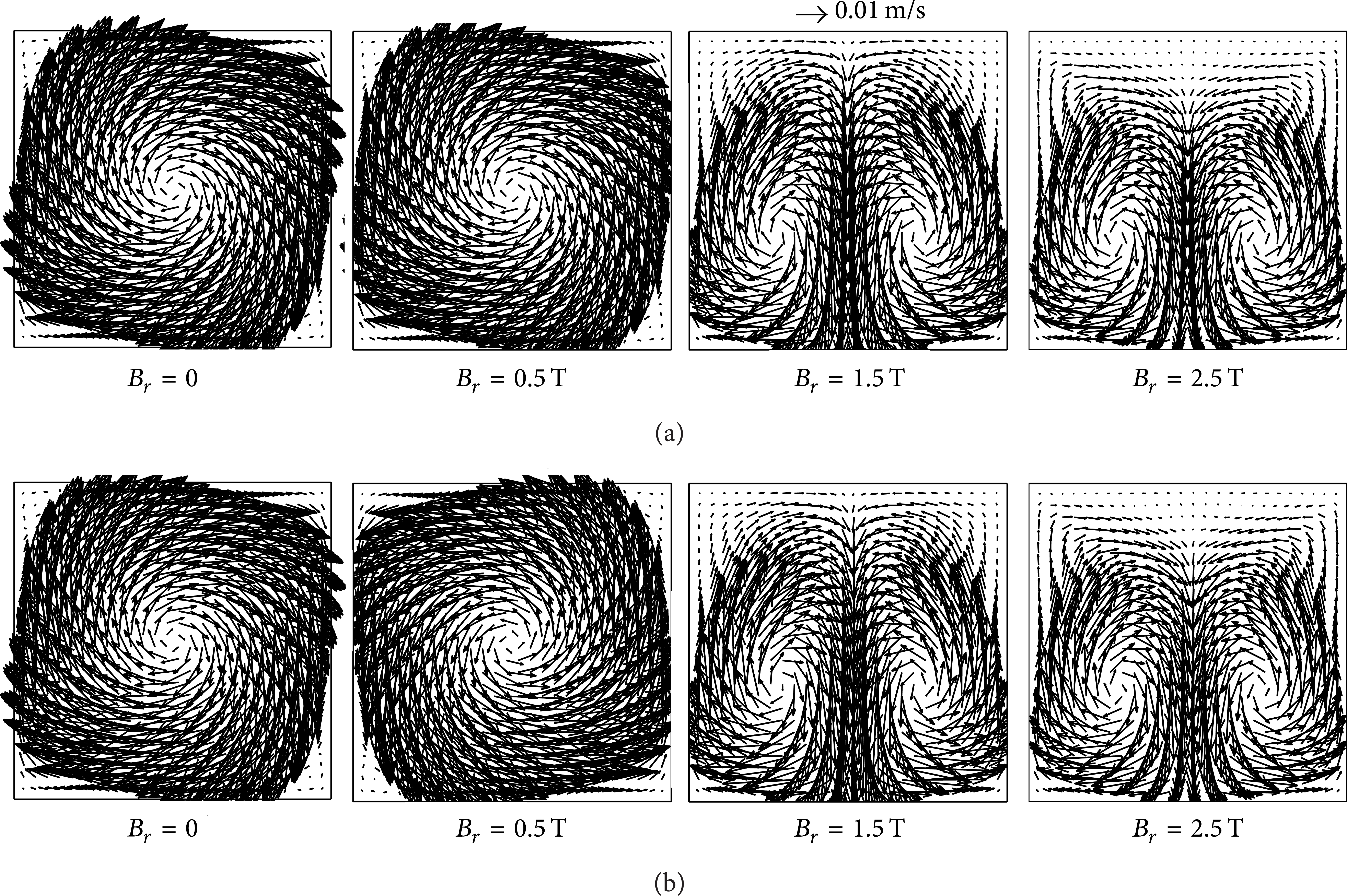
Velocity vectors of physical model PM-II with two types of magnetizing forces: (a) PM-II with FT-I and (b) PM-II with FT-II.

By comparing (15) with (17) we can find that the difference is the magnetic buoyancy force term. The curl of the magnetic buoyancy force term in (15) is

$\nabla \times \left(\frac{{\chi }_{\mathrm{0}}{\beta }_{\mathrm{0}}\left({\mathbf{B}}^{\mathrm{2}}\right)}{{\mu }_{\mathrm{0}}}\nabla \theta \right)=\frac{{\chi }_{\mathrm{0}}{\beta }_{\mathrm{0}}}{{\mu }_{\mathrm{0}}}\nabla {\mathbf{B}}^{\mathrm{2}}\times \nabla \theta .$

(27)

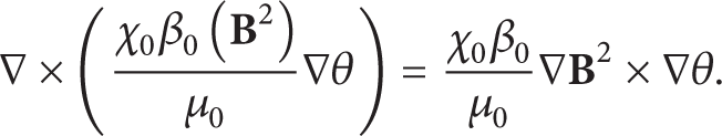
And the curl of the magnetic buoyancy force term in (17) is

$\nabla \times \left(-\frac{{\chi }_{\mathrm{0}}{\beta }_{\mathrm{0}}\left(\theta -{\theta }_{\mathrm{0}}\right)}{{\mu }_{\mathrm{0}}}\nabla {\mathbf{B}}^{\mathrm{2}}\right)=-\frac{{\chi }_{\mathrm{0}}{\beta }_{\mathrm{0}}}{{\mu }_{\mathrm{0}}}\nabla \theta \times \nabla {\mathbf{B}}^{\mathrm{2}}.$

(28)

One of the properties of the vector product is that the vector product is anticommutative; then,

$\nabla \theta \times \nabla {\mathbf{B}}^{\mathrm{2}}=-\nabla {\mathbf{B}}^{\mathrm{2}}\times \nabla \theta .$

(29)

Thus, the curl of the magnetic buoyancy term in (15) is equal to the curl of the magnetic buoyancy force term in (17). So the velocity field with magnetizing force type FT-I is the same as that with magnetizing force type FT-II for both physical models PM-I and PM-II. When we take curl of momentum equations (15) or (17), we get the vorticity equation with the same magnetic buoyancy force term and the same convection should result.

5.3. Comparison of Temperature Field

Figure 8 shows the temperature field with two types of magnetizing forces of physical model-I. When the magnetic field is B _r = 0.5 T, the effect of the magnetic field on the temperature field is weak, and the distribution of the temperature field is nearly the same as that when there is gravitation only, B _r = 0. With the increase of the magnetic field strength, the temperature fields change slightly. When the magnetic field is strong (B _r = 2.5 T), there is obvious change in the region near the top wall, and the temperature gradient increases in the corner adjacent to the top and cold walls. These are because a vortex is formed in the corner when B _r = 2.5 T as shown in Figure 6. For a physical model PM-I, the temperature field has similar distributions for both types of the magnetizing force. For PM-II, as the bottom wall is hot and the magnetic field is symmetric with respect to the central line in the computation domain both for the two magnetizing force types, the temperature fields are symmetric as shown in Figure 9 when B _r is 1.5 T and 2.5 T. But when the magnetic field is weak (B _r = 0.5 T), the temperature is not symmetric and the rotating direction is counterrotating for magnetizing force types I and II. It is because the magnetic field is so weak that the convection is more like the natural convection just under a gravity field (B _r = 0). This appears to reflect that the natural convection of physical model PM-II is physically unstable. The temperature fields of physical model-II are also quite similar to each other for different force types.

Figure 8:

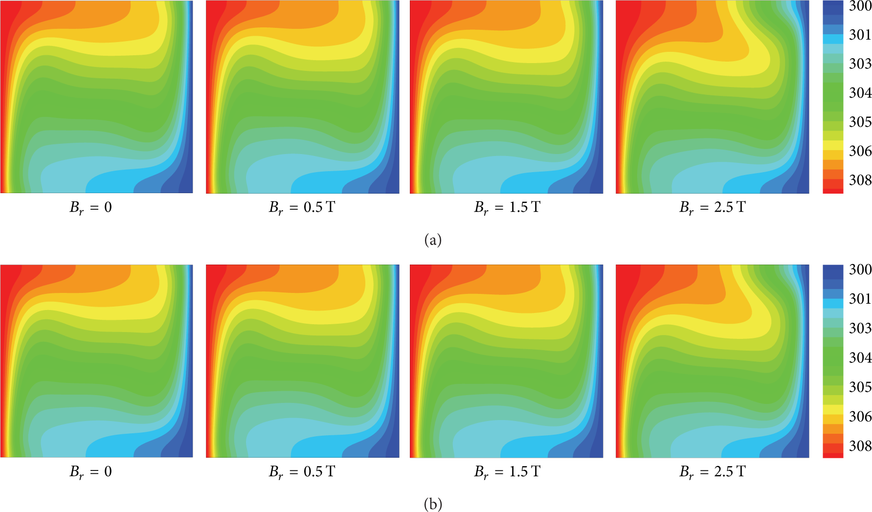
Temperature fields of physical model PM-I with two types of magnetizing forces: (a) PM-I with FT-I and (b) PM-I with FT-II.

Figure 9:

Temperature fields of physical model PM-II with two types of magnetizing forces: (a) PM-II with FT-I and (b) PM-II with FT-II.

Therefore, we can say that the temperature distributions are consistent for both physical models with two types of magnetizing forces even if they have quite different magnetizing force fields as shown in Figures 4 and 5. This is because the velocity fields are the same with two types of magnetizing forces.

5.4. Comparison of Local and Average Nu

The average Nusselt numbers on the hot wall for both models PM-I and PM-II are summarized in Table 3 under three different strengths of the magnetic fields. The value of average Nu decreases with increase of the strength of magnetic field. The values of average Nu relating to two types of magnetizing forces are nearly the same for both physical models, and the maximum difference is less than 0.6%. The curves of the local Nusselt number over the hot wall are shown in Figure 10 for physical models PM-I and PM-II. We can find that the local Nusselt numbers at the hot wall decrease with increase in the strength of the magnetic field. When the residual component of magnetic strength B _r is weak, that is, 0.5 T in this paper, the average Nusselt numbers are almost the same as that without a magnetic field. The values of Nusselt numbers under different magnetizing force types I and II are nearly the same for both models. For physical model II, as the model is physically unstable, the rotating direction of velocity field for the magnetizing force type I is contrary to that for the magnetizing force type II when B _r = 0.5 T, as shown in Figure 7. The distribution curves of the local Nusselt number are symmetrical with respect to the center of x (x/L = 0.5). This situation is justified as the natural convection without a magnetic field in model II is not ascertainable on the rotating direction due to its physical unstableness of physical model II. Thus, we can say that the cases with two different types of magnetizing forces have the same distribution curves of local Nusselt number along the hot wall for both models at three different residual flux densities of the permanent magnet.

Table 3:

Summary of computed results of two physical models with two magnetizing force types.

Model	B r	Nu (FT-I)	Nu (FT-II)
PM-I	0.5 T	4.506	4.505
	1.5 T	4.352	4.345
	2.5 T	3.898	3.920
PM-II	0.5 T	3.878	3.878
	1.5 T	3.006	3.024
	2.5 T	2.497	2.503

Figure 10:

Local Nusselt number along the hot wall. (a) PM-I with FT-I and FT-II; (b) PM-II with FT-I and FT-II.

6. Conclusion

Natural convection of air in a two-dimensional square enclosure under a nonuniform magnetic field of a permanent magnet placed above the enclosure is carried out. Two kinds of the expressions for the magnetizing force are considered. The magnetizing forces are quite different in the enclosure for the two different expressions of the magnetizing force, but the temperature field and the velocity fields are the same although the magnetizing force fields are different. The values of average Nusselt number and the distribution curves of local Nusselt number on the hot wall are also the same for the two magnetizing force expressions. The reason is that the curls of the magnetizing buoyancy force term for two types of magnetizing force are equal, so they have equivalent action on velocity fields although the magnetizing force fields are different. The numerical results reveal that the convection inside the enclosure does not depend on the types of expressions for magnetizing force in the region of residual magnetic flux density of a permanent magnet studied in this paper.