Coupling Two-Phase Fluid Flow with Two-Phase Darcy Flow in Anisotropic Porous Media

Abstract

This paper reports a numerical study of coupling two-phase fluid flow in a free fluid region with two-phase Darcy flow in a homogeneous and anisotropic porous medium region. The model consists of coupled Cahn-Hilliard and Navier-Stokes equations in the free fluid region and the two-phase Darcy law in the anisotropic porous medium region. A Robin-Robin domain decomposition method is used for the coupled Navier-Stokes and Darcy system with the generalized Beavers-Joseph-Saffman condition on the interface between the free flow and the porous media regions. Obtained results have shown the anisotropic properties effect on the velocity and pressure of the two-phase flow.

1. Introduction

Fluid flows in coupled free flow and porous media regions are of great interest and have several important applications, such as ground water systems [1], well-reservoir coupling in petroleum engineering [2], fluid-organ interactions, and industrial filtering where fluid passes through a filter to remove unwanted particles [3]. In the past two decades, there are many previous works addressing single-phase Stokes-Darcy system of single-phase flows [4–7] and the related problems such as Stokes-Navier Stokes systems [8, 9] and Stokes-Laplacian systems [1, 10]. However research of the two-phase flow in coupled free flow and porous media regions is still at a primary stage. Recently, the authors raise a numerical method for a model of two-phase flow in a coupled free flow and porous media system [11]. As far as we know, that paper is the first work on the two-phase flow in coupled free fluid and porous media regions. In that paper, we use a coupled Cahn-Hilliard and Navier-Stokes system to describe the two-phase fluid flow in the free flow region and two-phase Darcy equations to depict the Darcy flow in porous media region. A transmission condition for the two-phase flow is imposed at the interface boundary of the free flow region and the porous media region. For the single-phase flow, the Beavers-Joseph-Saffman (BJS) [12–14] condition states that the tangential slip velocity at the interface is proportional to the shear stress at the interface:

${\mathcal{L}}_p^{-\mathrm{1}}u=-\nu \frac{\partial u}{\partial n},$

(1)

where ${\mathcal{L}}_p$ is related to the permeability and the porosity of the porous media. For the two-phase flow, we expect that the slip velocity is proportional to the total stress at the fluid/porous media interface which, in addition to the fluid shear stress, should also consist of Young stress. Therefore a GNBC type of fluid/porous media interface condition (23) is proposed in this paper which is a natural generalization of the BJS condition. This interface condition is called the generalized Beavers-Joseph-Saffman (GBJS) condition.

In this paper, we consider coupling two-phase fluid flow in a free fluid region with two-phase Darcy flow in a homogeneous and anisotropic porous medium region. The anisotropic properties effect on the transportation of the two-phase flow is discussed. Anisotropy is generally a result of the orientation and shape of the asymmetric grains making up the porous bed. If the permeability of a porous medium varies with the direction of fluid flow or pressure gradient, the permeability is anisotropic. This variation in permeability with direction reflects the differences in path length through which a fluid element moves and the forces it experiences in moving through the porous media in a given direction. On the other hand, the permeability of a purely anisotropic media will not vary with position; that is, the media are homogeneous. In three-dimensional space, the directional nature of the permeability can be expressed as a symmetric second-order tensor with six independent components. Consider

$\mathbf{K}=\left(\begin{array}{ccc}{K}_{\mathrm{11}}& K_{\mathrm{12}}& K_{\mathrm{13}}\\ K_{\mathrm{12}}& K_{\mathrm{22}}& K_{\mathrm{23}}\\ K_{\mathrm{13}}& K_{\mathrm{23}}& K_{\mathrm{33}}\end{array}\right).$

(2)

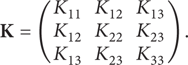
The transport properties of fluids in porous medium, such as reservoirs, are greatly influenced by the permeability of the medium.

The rest of the paper is organized as follows. We describe the modeling equations and the transmission conditions in Section 2. In Section 3, after a brief introduction of the numerical method for CH-NS system and IMPES method, we present the Robin-Robin domain decomposition method with GNBC transmission condition. Numerical examples together with some numerical analysis are presented in Section 4, where we highlight the anisotropic properties effect on transportation of the two-phase flow. A conclusion is presented in Section 5.

2. Modeling Equations

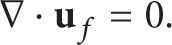
We consider the following situation: incompressible two-phase fluid in a region Ω _f flows across an interface Γ _I into a porous medium domain Ω _p as described in Figure 1. The model we used consists of coupled Cahn-Hilliard and Navier-Stokes equations for the free flow region Ω _f and a two-phase Darcy law for the two-phase flows in the porous medium region Ω _p . Let Ω _f and Ω _p denote bounded Lipschitz domains for the free flow region and the porous media region, respectively. The interface boundary between the domains is denoted by Γ _I : = ∂Ω _f ∩∂Ω _p . Let Ω: = Ω _f ∪Ω _p ∪Γ _I . The outward unit normal vectors to Ω _f and Ω _p are denoted by n _f and n _p , respectively. The tangent vectors on Γ _I are denoted as τ (for n = 2) or τ _l , l = 1, 2, (for n = 3).

Figure 1:

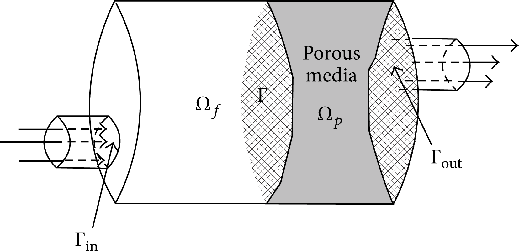
Illustration of flow domain.

We assume that there is an inflow boundary Γ_in, a subset of ∂Ω _f ∖Γ _I , which is separated from Γ _I and an outflow boundary Γ_out, a subset of ∂Ω _p ∖Γ _I , which is also separated from Γ _I . See Figure 1 for an illustration of the domain of the problem. Define Γ _f : = ∂Ω _f ∖(Γ _I ∪Γ_in) and Γ _p : = ∂Ω _p ∖(Γ _I ∪Γ_out).

2.1. The Coupled Cahn-Hilliard and Navier-Stokes Equations in the Free Flow Region

For free fluid region Ω _f , we assume that the two flow sytems is governed by a coupled system of Cahn-Hilliard Navier-Stokes equations, subject to a specified flow rate, q _f , across Γ_in. For simplicity we consider here the case of a single inflow boundary Γ_in:

$\begin{array}{c}\frac{\partial \varphi }{\partial t}+{\mathbf{u}}_f·\nabla \varphi =M\Delta \mu ,\\ \rho \left[\frac{\partial {\mathbf{u}}_f}{\partial t}+\left({\mathbf{u}}_f·\nabla \right){\mathbf{u}}_f\right]=-\nabla p_f+\nabla ·\mathbf{\sigma }+\mu \nabla \varphi +\rho g_{\text{ext}},\\ \nabla ·{\mathbf{u}}_f=\mathrm{0}.\end{array}$

(3)

Here p _f is the pressure in free fluid region; σ = ν(∇u _f + ∇u _f ^T ) denotes the viscous part of the stress tensor; ρ,ν are the fluid mass density and viscosity; ρg_ext is the external body force density; M is the phenomenological mobility coefficient; μ = − NΔϕ − rϕ + uϕ³ is the chemical potential; μ∇ϕ is the capillary force; N,r,u are the parameters that are related to the interface profile thickness $\xi =\sqrt{N/r}$ , the interfacial tension $\gamma =\mathrm{2}\sqrt{\mathrm{2}}{r}^{\mathrm{2}}\xi /\mathrm{3}u$ , and the two homogeneous equilibrium phases ${\varphi }_{\pm }=\pm \sqrt{r/u}$ .

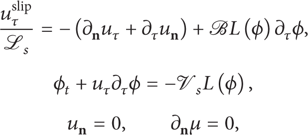
According to [15], the velocity along the solid boundary satisfies the GNBC:

$\beta u_{\tau }^{\text{slip}}=-\nu \left({\partial }_{\mathbf{n}}{u}_{\tau }+{\partial }_{\tau }{u}_{\mathbf{n}}\right)+L\left(\varphi \right){\partial }_{\tau }\varphi ,$

(4)

where L(ϕ) = N∂ _n ϕ + ∂γ _ωf (ϕ)/∂ϕ, γ _ωf (ϕ) = − (1/2)γcos⁡θ _s sin((π/2)ϕ)), θ _s is the static contact angle, and u _n and u_τ are the normal velocity and tangent velocity, respectively, where n and τ are the unit normal and tangent vectors of the slip boundary. In addition, a dynamic boundary condition is imposed on the phase field variable ϕ at the slip boundary. Consider

$\frac{\partial \varphi }{\partial t}+u_{\tau }{\partial }_{\tau }\varphi =-\Pi L\left(\varphi \right),$

(5)

where Π is a phenomenological parameter and should be positive. And also, the following nonpenetration boundary conditions are used on Γ _f . Consider

$u_{\mathbf{n}}={\mathbf{u}}_f·{\mathbf{n}}_f=\mathrm{0},\hspace{1em}\hspace{1em}{\partial }_{\mathbf{n}}\mu =\mathrm{0}.$

(6)

Following [15], we scale length by a reference length L, velocity by the reference velocity V, time by L/V, and pressure by V/L, and the following dimensionless equations are obtained:

$\frac{\partial \varphi }{\partial t}+{\mathbf{u}}_f·\nabla \varphi ={\mathcal{L}}_d\Delta \mu ,$

(7)

$\mathcal{R}\left[\frac{\partial {\mathbf{u}}_f}{\partial t}+\left({\mathbf{u}}_f·\nabla \right){\mathbf{u}}_f\right]=-\nabla p_f+\nabla ·\mathbf{\sigma }+\mathcal{B}\mu \nabla \varphi ,$

(8)

$\nabla ·{\mathbf{u}}_f=\mathrm{0}.$

(9)

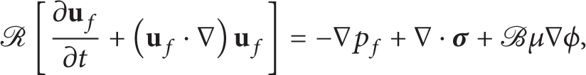
Here μ = − ϵΔϕ − ϕ/ϵ + ϕ³/ϵ is the chemical potential; ϵ is the ratio between dynamic interface thickness ξ and characteristic length L; σ = ν(∇u _f + ∇u _f ^T ) is the viscous part of the stress tensor. For the convenience of imposing coupling conditions on the interface Γ _I , we keep stress tensor in the diffusion term and do not divide viscosity ν on both sides of Navier-Stokes equation (8). Notice that we have neglected external body force here, which can be easily incorporated into the above equations. The boundary conditions at top and bottom walls are as follows:

$\begin{array}{c}\frac{u_{\tau }^{\text{slip}}}{{\mathcal{L}}_s}=-\left({\partial }_{\mathbf{n}}{u}_{\tau }+{\partial }_{\tau }{u}_{\mathbf{n}}\right)+\mathcal{B}L\left(\varphi \right){\partial }_{\tau }\varphi ,\\ {\varphi }_t+u_{\tau }{\partial }_{\tau }\varphi =-{\mathcal{V}}_{s}L\left(\varphi \right),\\ u_{\mathbf{n}}=\mathrm{0},\hspace{1em}\hspace{1em}{\partial }_{\mathbf{n}}\mu =\mathrm{0},\end{array}$

(10)

where $L(\varphi )=ϵ{\partial }_{\mathbf{n}}\varphi -(\sqrt{\mathrm{2}}/\mathrm{6})\pi \cos {\theta }_s\cos ((\pi /\mathrm{2})\varphi )$ . Six dimensionless parameters appear in the above equations. They are (1) $\mathrm{\hspace{0.17em}\hspace{0.17em}}{\mathcal{L}}_d=\mathrm{3}M\gamma /\mathrm{2}\sqrt{\mathrm{2}}V{L}^{\mathrm{2}}$ , (2) $\mathcal{R}=\rho VL$ , (3) $\mathcal{B}=\mathrm{3}\gamma /\mathrm{2}\sqrt{\mathrm{2}}V$ , (4) $\mathrm{\hspace{0.17em}\hspace{0.17em}}{\mathcal{V}}_s=\mathrm{3}\gamma \Pi L/\mathrm{2}\sqrt{\mathrm{2}}V$ , and (5) ${\mathcal{L}}_s=\nu /\beta (\varphi )L$ , which is the ratio of the slip length l _s (ϕ) = ν/β(ϕ) to L, and (6) ϵ, which is the ratio between interface thickness ξ and characteristic length L.

2.2. Darcy's Law for the Two-Phase Flows in the Anisotropic Porous Media Region

In Ω _p , we assume that the flow is governed by the following system, where the wetting phase is indicated by a subscript w and the nonwetting phase is indicated by o. The mass balance equation for each of the fluid phases is as follows:

$\phi \frac{\partial \left({\rho }_{\alpha }{S}_{\alpha }\right)}{\partial t}+\nabla ·\left({\rho }_{\alpha }{\mathbf{u}}_{\alpha }\right)=\mathrm{0},\hspace{1em}\alpha =w,o,$

(11)

where φ is the porosity of the medium and ρ_α, S_α, and u_α are the density, saturation, and volumetric velocity of the α-phase, respectively. The volumetric velocity u_α is given by Darcy's law. Consider

${\mathbf{u}}_{\alpha }=-\frac{K_{r\alpha }}{{\nu }_{\alpha }}\mathbf{K}\nabla \left(p_{\alpha }-{\rho }_{\alpha }{g}_{\text{ext}}Z\right),\hspace{1em}\mathrm{\hspace{0.17em}\hspace{0.17em}}\alpha =w,o,$

(12)

where K is the absolute permeability of the anisotropic porous medium, which is a symmetric second-order tensor. p_α, ν_α, and K _rα are the pressure, viscosity, and relative permeability of the α-phase, respectively. g_ext is the gravitational constant and the z-coordinate is in the vertical downward direction. The constraint for the saturations is

$S_w+S_o=\mathrm{1},$

(13)

and the two pressures are related by a given capillary pressure function. Consider

$p_c\left(S_w\right)=p_o-p_w.$

(14)

Equations (11)–(14) are called phase formulations for two-phase flows in the porous media region. For the convenience of assigning transmission conditions, we introduce the global pressure [16] into the model, which is defined as follows:

$p\left(S_w\right)=p_o-{{\displaystyle \int }}_{S_{\mathrm{0}}}^{S_w}‍f_w\left(\xi \right)p_c^{\prime }\left(\xi \right)\text{d}\xi +{\pi }_{\mathrm{0}},$

(15)

where S₀, π₀ are constants to be chosen and f _w are fractional function of wetting phase defined in (28). Since the global pressure is related to the phase pressures, constants S₀, π₀ can be fixed as follows:

$S_{\mathrm{0}}=\mathrm{1}-S_{or},\hspace{1em}\hspace{1em}{\pi }_{\mathrm{0}}=p_c\left(\mathrm{1}-S_{or}\right),$

(16)

with S _or being the nonwetting phase residual saturation.

At last, the model is completed by specifying boundary and initial conditions. The boundary conditions on Γ _p are as follows:

${\mathbf{u}}_{\alpha }·{\mathbf{n}}_p=\mathrm{0},\hspace{1em}\alpha =w,o.$

(17)

The initial condition is given by

$S\left(\mathbf{x},\mathrm{0}\right)=S^{\mathrm{0}}\left(\mathbf{x}\right).$

(18)

2.3. Transmission Conditions

To couple the two flow systems, several transmission conditions are imposed on the interface boundary Γ _I . They are conservation of mass. Consider

${\mathbf{u}}_f·{\mathbf{n}}_f+\mathbf{u}·{\mathbf{n}}_p=\mathrm{0},$

(19)

where u = u _w + u _o is the total velocity in porous domain. This condition guarantees the continuity of normal velocity across interface. The traction vector t is the force on Γ _I acting on the fluid volume inside Ω _f . Consider

$\mathbf{t}\left({\mathbf{u}}_f,p_f\right)=\mathbf{T}\left({\mathbf{u}}_f,p_f\right)·{\mathbf{n}}_f,$

(20)

where $\mathbf{T}({\mathbf{u}}_f,p_f)\triangleq -p_f\mathbb{I}+\nu (\nabla \mathbf{u}+\nabla {\mathbf{u}}^T)$ is the stress tensor. The force on Γ _I exerted by the fluid volume is − t. The force in Ω _p acting on Γ _I is the global pressure p. Continuity of forces gives

$-\mathbf{t}\left({\mathbf{u}}_f,p_f\right)·{\mathbf{n}}_f=p.$

(21)

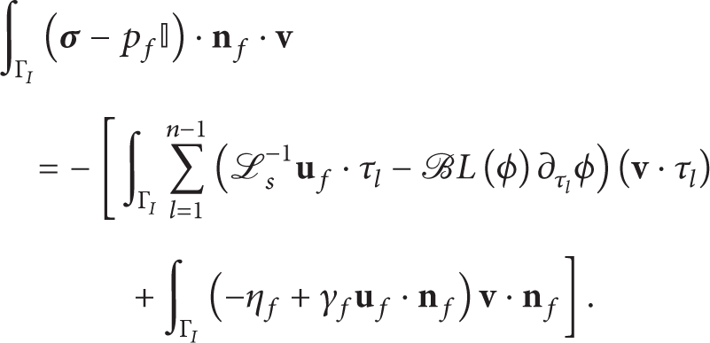
This gives the balance of the normal forces across the interface:

$p_f-\left(\mathbf{\sigma }·{\mathbf{n}}_f\right)·{\mathbf{n}}_f=p.$

(22)

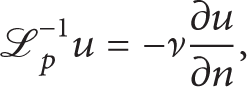
We then propose the generalized Beavers-Joseph-Saffman (GBJS) condition on the interface Γ _I :

${\mathcal{L}}_p^{-\mathrm{1}}{\mathbf{u}}_f·{\tau }_l=-{\tau }_l·\mathbf{\sigma }·{\mathbf{n}}_f+\mathcal{B}L\left(\varphi \right){\partial }_{{\tau }_l}\varphi ,\hspace{1em}l=\mathrm{1},\dots ,n-\mathrm{1},$

(23)

which is a natural generalization of GNBC and it states that the slip velocity along Γ _I is proportional to the sum of tangential viscous stress and the interfacial Young stress [15]. Here coefficient ${\mathcal{L}}_p^{-\mathrm{1}}=C/\sqrt{\text{trace}(\mathbf{K})}$ , according to [14].

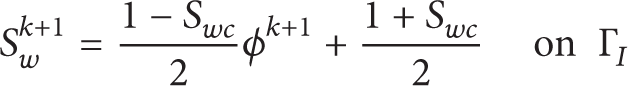
In the porous media domain, there is an irreducible saturation [2], which means at this value the wetting phase can no longer be displaced by applying a pressure gradient. As a consequence, the phase profile ϕ and saturation S _w are supposed to satisfy the following relation when the flow across Γ _I :

$S_w\mathbf{u}·{\mathbf{n}}_p=-\left(\frac{\mathrm{1}-S_{wc}}{\mathrm{2}}\varphi +\frac{\mathrm{1}+S_{wc}}{\mathrm{2}}\right){\mathbf{u}}_f·{\mathbf{n}}_f,$

(24)

where S _wc is irreducible saturation and ϕ = 1 corresponds to the wetting phase. From (19), we then have

$S_w=\left(\frac{\mathrm{1}-S_{wc}}{\mathrm{2}}\varphi +\frac{\mathrm{1}+S_{wc}}{\mathrm{2}}\right).$

(25)

Overall, transmission conditions (19), (22), (23), and (25) are imposed on Γ _I and ∂ _n μ = 0 is imposed on Γ _I for the coupled Cahn-Hilliard Navier-Stokes system, which means the chemical potential does not change along the normal direction on the boundary.

3. The Numerical Method

In this section, we introduce the numerical method to solve the model of two-phase flow in a coupled free flow and porous media system. This numerical method is firstly introduced in [11]. Here we just describe the framework of this method and highlight the difference caused by anisotropic property of porous media.

3.1. Numerical Method for the Coupled Cahn-Hilliard and Navier-Stokes Equations

A semi-implicit temporal discretization with a convex splitting scheme is employed to solve Cahn-Hilliard equation. Given ϕ ⁿ ,u _n and the time step δt = t^{n + 1} − t ⁿ , we solve for ϕ^{n + 1}, μ^{n + 1}, p^{n + 1}, and u_{n + 1} in two steps.

1. Solve the Cahn-Hilliard equations with the semi-implicit method and finite element discretization to obtain ϕ^{n + 1} and μ^{n + 1} with a convex splitting scheme. The scheme employed is unconditionally stable under some conditions.

2. With the obtained ϕ^{n + 1} and μ^{n + 1}, the Navier-Stokes equations are solved with a P2-P0 mixed finite element method. Here, for the nonlinear term, we use the linearized semi-implicit temporal discretization to avoid the nonlinear iteration.

For details of the scheme, see [17, 18].

3.2. IMPES Method for the Two-Phase Darcy Law

We introduce the phase mobility functions

${\lambda }_{\alpha }\left(\mathbf{x},S\right)=\frac{K_{r\alpha }}{{\nu }_{\alpha }},\hspace{1em}\alpha =w,o,$

(26)

and the total mobility

$\lambda \left(\mathbf{x},S\right)={\lambda }_w+{\lambda }_o,$

(27)

where S = S _w . The fractional flow functions are defined by

$f_{\alpha }\left(\mathbf{x},S\right)=\frac{{\lambda }_{\alpha }}{\lambda },\hspace{1em}\alpha =w,o.$

(28)

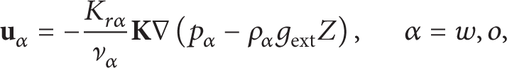
We use the global pressure p as the pressure variable and define the total velocity by

$\mathbf{u}={\mathbf{u}}_w+{\mathbf{u}}_o.$

(29)

Under the assumption that the fluids are incompressible and substitute (13) and (29) into (11), we have

$\nabla ·\mathbf{u}=\mathrm{0}.$

(30)

Substitute (14) and (29) into (12) to obtain

$\mathbf{u}=-\mathbf{K}\left(\lambda \left(S\right)\nabla p-{\lambda }_w\left(S\right)\nabla p_c-\left({\lambda }_w{\rho }_w+{\lambda }_o{\rho }_o\right)g\nabla Z\right).$

(31)

From the definition of global pressure (15), we get

$\nabla p=\nabla p_o-f_w\nabla p_c.$

(32)

This is equivalent to

$\lambda \nabla p={\lambda }_w\nabla p_w+{\lambda }_o\nabla p_o,$

(33)

which implies that the global pressure is the pressure that would produce flow of a fluid with mobility λ equal to the sum of the flows of fluids w and o. Substitute (32) into (31) to have

$\mathbf{u}=-\mathbf{K}\left(\lambda \left(S\right)\nabla p-\left({\lambda }_w{\rho }_w+{\lambda }_o{\rho }_o\right)g\nabla Z\right).$

(34)

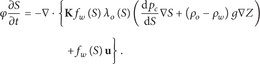
Similarly, apply (14), (29), and (34) to (11) and (12) with α = w to have the saturation equation:

$\phi \frac{\partial S}{\partial t}=-\nabla ·\{\mathbf{K}{f}_w\left(S\right){\lambda }_o\left(S\right)\left(\frac{\text{d}{p}_c}{\text{d}S}\nabla S+\left({\rho }_o-{\rho }_w\right)g\nabla Z\right)\hspace{0.5em}+f_w\left(S\right)\mathbf{u}\phantom{\left(\frac{\text{d}{p}_c}{\text{d}S}\nabla S+\left({\rho }_o-{\rho }_w\right)g\nabla Z\right)}\}.$

(35)

We substitute (34) into (30) to give the pressure equation:

$-\nabla ·(\mathbf{K}\lambda \nabla p)=-\nabla ·\left(\mathbf{K}\left({\lambda }_w{\rho }_w+{\lambda }_o{\rho }_o\right)g\nabla Z\right).$

(36)

Let J = (0,T)(T > 0) be the time interval of interest, and for a positive integer N, let 0 = t⁰ < t¹ < ⋯ < t ^N = T be a partition of J. Now, the IMPES method goes as follows. Given S ⁿ , we solve pressure p ⁿ from (36); that is,

$-\nabla ·\left(\mathbf{K}\lambda \left(S^n\right)\nabla p^n\right)=F\left(p^n,S^n\right),$

(37)

where F(p,S) denotes the right-hand side of (36). For anisotropic porous media, when IMPES method is employed to solve the two-phase Darcy equations, we need to solve a second-order elliptic equation with a second-order tensor diffusion coefficient. S^{n + 1} is then updated explicitly from (35); that is,

$\phi \frac{S^{n+\mathrm{1}}-S^n}{\Delta t}=G\left(p^n,{\mathbf{u}}^n,S^n\right),$

(38)

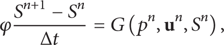
where G(p,u,S) represents the right-hand side of (35).

3.3. Weak Form of the Coupled Problem and the Robin-Robin Iterative Method

For simplicity, we neglect the capillary pressure and gravitational term in the Darcy law of two-phase flows. Since the coupling conditions are related to − ∇p _f + ∇·σ in Navier-Stokes equation, we deduce the weak form for these two terms in detail. Letting ${\text{X}}_f=\left\{v:v\in {\left(H^1\left({\Omega }_f\right)\right)}^n,v|{\Gamma }_{f,D}=0\right\}$ , we multiply these two terms by a vector function v ∈ X _f and integrate over Ω _f to obtain

${{\displaystyle \int }}_{{\Omega }_f}\left(-\nabla p_f+\nabla ·\mathbf{\sigma }\right)·\mathbf{v}\hspace{1em}={{\displaystyle \int }}_{{\Omega }_f}‍p_f\nabla ·\mathbf{v}-{{\displaystyle \int }}_{{\Omega }_f}‍\mathbf{\sigma }:D\left(\mathbf{v}\right)\hspace{1em}+{{\displaystyle \int }}_{\partial {\Omega }_f}‍\mathbf{\sigma }·{\mathbf{n}}_f·\mathbf{v}-{{\displaystyle \int }}_{\partial {\Omega }_f}‍p_f\mathbb{I}·{\mathbf{n}}_f·\mathbf{v},$

(39)

where D(v) = (1/2)(∇v + ∇v _T ) and $\mathbb{I}$ is an identity matrix. We focus on the interface Γ _I and notice the fact that {n _f ,τ _l ,l = 1,…,n − 1} form an orthogonal basis; therefore

${{\displaystyle \int }}_{{\Gamma }_I}\left(\mathbf{\sigma }-p_f\mathbb{I}\right)·{\mathbf{n}}_f·\mathbf{v}\hspace{1em}=-[{{\displaystyle \int }}_{{\Gamma }_I}{\displaystyle \sum }_{l=\mathrm{1}}^{n-\mathrm{1}}‍\left({\mathcal{L}}_s^{-\mathrm{1}}{\mathbf{u}}_f·{\tau }_l-\mathcal{B}L\left(\varphi \right){\partial }_{{\tau }_l}\varphi \right)\left(\mathbf{v}·{\tau }_l\right)\hspace{1em}\hspace{0.5em}+{{\displaystyle \int }}_{{\Gamma }_I}p\mathbf{v}·{\mathbf{n}}_f].$

(40)

Recall that we need to solve the following Poisson equation in the porous domain and we neglect the gravitational term on the right-hand side of (36), which becomes

$-\nabla ·\left(\mathbf{K}\lambda \nabla p\right)=\mathrm{0},$

(41)

where λ is the total mobility. Let X _p = {ψ:ψ ∈ H¹(Ω _p ),ψ|_Γp,D = 0}. We multiply (41) by a scalar function ψ ∈ X _p and integrate over Ω _p to obtain

${{\displaystyle \int }}_{{\Omega }_p}\mathbf{K}\lambda \nabla p·\nabla \psi -{{\displaystyle \int }}_{\partial {\Omega }_p}\mathbf{K}\lambda \nabla p·{\mathbf{n}}_p\psi =\mathrm{0}.$

(42)

Recalling that u = − Kλ∇p _o , we have

${{\displaystyle \int }}_{{\Omega }_p}\mathbf{K}\lambda \nabla p·\nabla \psi +{{\displaystyle \int }}_{{\Gamma }_I}\mathbf{u}·{\mathbf{n}}_p\psi =\mathrm{0}.$

(43)

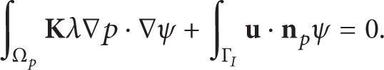
To solve the CH-NS and Darcy system, we adopt the idea of Robin-Robin algorithm, which is well known in domain decomposition method [9]. Let us consider the following Robin condition for the flow region: for a given constant γ _f > 0 and a given function η _f defined on Γ _I ,

$\left({\mathbf{n}}_f·\left(\mathbf{\sigma }·{\mathbf{n}}_f\right)-p_f\right)+{\gamma }_f{\mathbf{u}}_f·{\mathbf{n}}_f={\eta }_f\hspace{1em}\mathrm{on}\mathrm{\hspace{0.17em}\hspace{0.17em}}{\Gamma }_I.$

(44)

Then, (40) is converted into

${{\displaystyle \int }}_{{\Gamma }_I}\left(\mathbf{\sigma }-p_f\mathbb{I}\right)·{\mathbf{n}}_f·\mathbf{v}\hspace{1em}=-[{{\displaystyle \int }}_{{\Gamma }_I}{\displaystyle \sum }_{l=\mathrm{1}}^{n-\mathrm{1}}\left({\mathcal{L}}_s^{-\mathrm{1}}{\mathbf{u}}_f·{\tau }_l-\mathcal{B}L\left(\varphi \right){\partial }_{{\tau }_l}\varphi \right)\left(\mathbf{v}·{\tau }_l\right)\hspace{1em}\hspace{0.5em}+{{\displaystyle \int }}_{{\Gamma }_I}\left(-{\eta }_f+{\gamma }_f{\mathbf{u}}_f·{\mathbf{n}}_f\right)\mathbf{v}·{\mathbf{n}}_f].$

(45)

Let (·,·)_Ω denote the L² inner product on the domain Ω, and 〈·,·〉 denotes the L² inner product on the interface Γ _I . Then, the corresponding weak formulation for the CH-NS system in the flow domain is given by the following: for η _f ∈ L²(Γ _I ), find (u _f ,p _f ,ϕ,μ) ∈ X _f ′ × L²(Ω _f ) × H¹(Ω _f ) × H¹(Ω _f ) such that

$\begin{array}{c}\mathcal{R}{\left(\frac{\partial {\mathbf{u}}_f}{\partial t},\mathbf{v}\right)}_{{\Omega }_f}+\mathcal{R}{\left(\left({\mathbf{u}}_f·\nabla \right){\mathbf{u}}_f,\mathbf{v}\right)}_{{\Omega }_f}\hspace{1em}+{{\displaystyle \int }}_{{\Omega }_f}\mathbf{\sigma }:D\left(\mathbf{v}\right)-{\left(p_f,\nabla ·\mathbf{v}\right)}_{{\Omega }_f}\hspace{1em}+{\displaystyle \sum }_{l=\mathrm{1}}^{n-\mathrm{1}}〈{\mathcal{L}}_s^{-\mathrm{1}}{\mathbf{u}}_f·{\tau }_l-\mathcal{B}L\left(\varphi \right){\partial }_{{\tau }_l}\varphi ,\mathbf{v}·{\tau }_l〉\hspace{1em}+〈-{\eta }_f+{\gamma }_f{\mathbf{u}}_f·{\mathbf{n}}_f,\mathbf{v}·{\mathbf{n}}_f〉\hspace{1em}-\mathcal{B}{\left(\mu \nabla \varphi ,\mathbf{v}\right)}_{{\Omega }_f}=\mathrm{0},\\ {\left(\nabla ·{\mathbf{u}}_f,q_f\right)}_{{\Omega }_f}=\mathrm{0},\\ {\left(\frac{\partial \varphi }{\partial t},\chi \right)}_{{\Omega }_f}-{\left(\varphi {\mathbf{u}}_f,\nabla \chi \right)}_{{\Omega }_f}+{\mathcal{L}}_d{\left(\nabla \mu ,\nabla \chi \right)}_{{\Omega }_f}=\mathrm{0},\\ {\left(\mu ,\chi \right)}_{{\Omega }_f}=ϵ{\left(\nabla \varphi ,\nabla \chi \right)}_{{\Omega }_f}-\frac{\mathrm{1}}{ϵ}{\left(\varphi -{\varphi }^{\mathrm{3}},\chi \right)}_{{\Omega }_f},\\ \forall \left(\mathbf{v},q_f,\chi \right)\in {\mathbf{X}}_f\times H^{\mathrm{1}}\left({\Omega }_f\right)\times H^{\mathrm{1}}\left({\Omega }_f\right),\end{array}$

(46)

where X _f ′ = {v:v ∈ (H¹(Ω _f )) ⁿ ,v|_Γf,D = v_in} and v_in is the velocity imposed on the left boundary Γ_in.

Similarly, we propose the following Robin type condition for the porous domain: for a given constant γ _p > 0 and a given function η _p defined on Γ _I ,

$-{\gamma }_p\mathbf{u}·{\mathbf{n}}_p+p={\eta }_p\hspace{1em}\mathrm{on}\mathrm{\hspace{0.17em}\hspace{0.17em}}{\Gamma }_I.$

(47)

Then, the corresponding weak formulation for the pressure equation (41) is given by the following: for η _p ∈ L²(Γ _I ), find p ∈ X _p ′ such that

${\gamma }_p{\left(\mathbf{K}\lambda \nabla p,\nabla \psi \right)}_{{\Omega }_p}+〈p,\psi 〉=〈{\eta }_p,\psi 〉,\hspace{1em}\forall \psi \in {\mathbf{X}}_p,$

(48)

where X _p ′ = {ψ:ψ ∈ H¹(Ω _f ),ψ|_Γp,D = p_out} and p_out is the pressure imposed on the right boundary Γ_out. Then use

$\phi \frac{\partial S}{\partial t}=G$

(49)

to update the saturation S, where the right-hand side function G = − u·∇f _w (S). Here the gradient must be discretized in upwind schemes.

Given initial values η _f ⁰ and η _p ⁰ which may be taken to be zeroes, η _f ^{k + 1} and η _p ^{k + 1} are updated in the following manner:

$\begin{array}{c}{\eta }_f^{k+\mathrm{1}}=a{\eta }_p^k+b{p}^k,\\ {\eta }_p^{k+\mathrm{1}}=c{\eta }_f^k+d{\mathbf{u}}_f^k·{\mathbf{n}}_f.\end{array}$

(50)

We suppose that η _f ^k and η _p ^k converge to η _f * and η _p *, respectively, and p ^k and u _f ^k also converge to the true solution p* and u _f *, respectively. Then, by (50), we have

$\begin{array}{c}{\eta }_f^{*}=a{\eta }_p^{*}+b{p}^{*}={\gamma }_f{\mathbf{u}}_f^{*}·{\mathbf{n}}_f-p^{*},\\ {\eta }_p^{*}=c{\eta }_f^{*}+d{\mathbf{u}}_f^{*}·{\mathbf{n}}_f={\gamma }_p{\mathbf{u}}_f^{*}·{\mathbf{n}}_f+p^{*},\end{array}$

(51)

which leads to a choice of coefficients a, b, c, and d as follows:

$\begin{array}{c}a=\frac{{\gamma }_f}{{\gamma }_p},\hspace{1em}\hspace{1em}b=-\mathrm{1}-a,\\ c=-\mathrm{1},\hspace{1em}\hspace{1em}d={\gamma }_f+{\gamma }_p.\end{array}$

(52)

Since the flow is from the free flow region to the porous media region, we use (25) to update the saturation S _w on the interface Γ _I ; that is,

$S_w^{k+\mathrm{1}}=\frac{\mathrm{1}-S_{wc}}{\mathrm{2}}{\varphi }^{k+\mathrm{1}}+\frac{\mathrm{1}+S_{wc}}{\mathrm{2}}\hspace{1em}\mathrm{on}\mathrm{\hspace{0.17em}\hspace{0.17em}}{\Gamma }_I$

(53)

and then is used as the boundary condition for (38). Now we describe the domain decomposition algorithm used in this paper. Define

${\xi }_{{\Gamma }_I}={\parallel \left({\mathbf{u}}_f-\mathbf{u}\right)·{\mathbf{n}}_f\parallel }_{L^{\mathrm{2}}\left({\Gamma }_I\right)}$

(54)

as an indicator and assuming that the interval [0,T] is partitioned into N equal intervals of length δt = T/N, where the uniformity of the partition is not essential to the algorithm, the algorithm proceeds as follows.

Algorithm 1 (Robin-Robin domain decomposition algorithm). Given a tolerance $\mathtt{T}\mathtt{O}\mathtt{L}>\mathrm{0}$ .

• Give initial values to η _f and η _p , usually set η _f ⁰ = 0, η _p ⁰ = 0. Set iteration index k = 0.

• For n = 0, 1,…,N − 1,

4. Numerical Results

In this section, two numerical examples are presented to validate our model and numerical scheme. The first example is a droplet of nonwetting phase passing through the interface, which corresponds to a drainage procedure. The second example is a layer of nonwetting phase passing through the interface, which corresponds to an imbibition procedure. For both examples, isotropic and anisotropic porous media are simulated to make comparisons. In the second example, the dynamic interface intersects with both the upper and lower boundaries as well as the interface boundary Γ _I .

For both examples, the computational domain is Ω = [0, 2] × [0, 1], in which the free flow region is Ω _f = [0, 1] × [0, 1] and the porous media region is Ω _p = [1, 2] × [0, 1]. A uniform triangular mesh is used and the meshes on the interface are matching.

The following empirical formulas of relative permeability are used in both examples:

$\begin{array}{c}{K}_{rw}={\left(\frac{S_w-S_{wc}}{\mathrm{1}-S_{wc}-S_{or}}\right)}^{\mathrm{2}},\\ K_{ro}={\left(\frac{\mathrm{1}-S_w-S_{or}}{\mathrm{1}-S_{wc}-S_{or}}\right)}^{\mathrm{2}},\end{array}$

(55)

where S _wc is irreducible saturation and S _or is the nonwetting phase residual saturation.

4.1. A Droplet Passing through Interface

A droplet of nonwetting phase is put in the free flow region initially at {[x,y] ∣ (x − 0.75)² + (y − 0.5)² ≤ 0.2²}. ϕ⁰ = − 1 inside the droplet and ϕ⁰ = 1 outside the droplet. The initial saturation S⁰ in the porous media region is set to 1. The time step used is dt = 0.1 × h, where h is the edge length of the triangle elements and h = 1/50.

According to [14], the slip coefficient ${\mathcal{L}}_p^{-\mathrm{1}}=C/\sqrt{\text{trace}(\mathbf{K})}$ on the interface, where C is a dimensionless constant and it is chosen to be 0.1 for flow in a channel with a permeable wall. As a consequence, the slip coefficient is much larger on the interface than on the normal boundary.

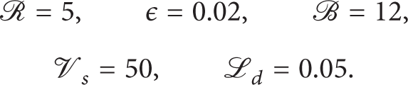
The parameters used in the CH-NS equations are listed as follows:

$\begin{array}{c}\mathcal{R}=\mathrm{5},\hspace{1em}\hspace{1em}ϵ=\mathrm{0.02},\hspace{1em}\hspace{1em}\mathcal{B}=\mathrm{12},\\ {\mathcal{V}}_s=\mathrm{50},\hspace{1em}\hspace{1em}{\mathcal{L}}_d=\mathrm{0.05}.\end{array}$

(56)

On the top and bottom boundaries, the slip coefficient and the static contact angle are chosen to be

${\mathcal{L}}_s=\mathrm{0.0038},\hspace{1em}\hspace{1em}{\theta }_s=\mathrm{6}{\mathrm{0}}^{°}.$

(57)

On the interface Γ _I , they are

${\mathcal{L}}_p=\mathrm{14.83},\hspace{1em}\hspace{1em}{\theta }_s=\mathrm{6}{\mathrm{0}}^{°}.$

(58)

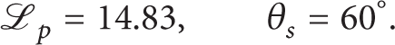
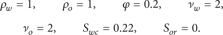
The parameters used in the Darcy law are listed as follows:

$\begin{array}{c}{\rho }_w=\mathrm{1},\hspace{1em}\hspace{1em}{\rho }_o=\mathrm{1},\hspace{1em}\hspace{1em}\phi =\mathrm{0.2},\hspace{1em}\hspace{1em}{\nu }_w=\mathrm{2},\\ {\nu }_o=\mathrm{2},\hspace{1em}\hspace{1em}\mathrm{\hspace{0.17em}\hspace{0.17em}}{S}_{wc}=\mathrm{0.22},\hspace{1em}\hspace{1em}\mathrm{\hspace{0.17em}\hspace{0.17em}}{S}_{or}=\mathrm{0}.\end{array}$

(59)

The absolute permeability is

$\mathbf{K}\mathbf{=}\left(\begin{array}{cc}\cos \left(-\alpha \right)& \sin \left(-\alpha \right)\\ -\sin \left(-\alpha \right)& \cos \left(-\alpha \right)\end{array}\right)\left(\begin{array}{cc}\mathrm{2.00}& \mathrm{0.00}\\ \mathrm{0.00}& \mathrm{0.20}\end{array}\right)\hspace{1em}\times \left(\begin{array}{cc}\cos \left(-\alpha \right)& \sin \left(-\alpha \right)\\ -\sin \left(-\alpha \right)& \cos \left(-\alpha \right)\end{array}\right)=\left(\begin{array}{cc}\mathrm{1.55}& \mathrm{0.78}\\ \mathrm{0.78}& \mathrm{0.65}\end{array}\right),$

(60)

where α = π/6; that is, the angle between the principle direction and X-axis is 30 degrees. A parabolic velocity field is put on Γ_in (left boundary), and to avoid the whole system being singular, a pressure is assigned on Γ_out (right boundary).

The parameters used for iteration are listed as follows:

${\gamma }_f=\mathrm{0.2},\hspace{1em}\hspace{1em}{\gamma }_p=\mathrm{0.2},\hspace{1em}\hspace{1em}{\eta }_f^{\mathrm{0}}=\mathrm{0},\hspace{1em}\hspace{1em}{\eta }_p^{\mathrm{0}}=\mathrm{0}.$

(61)

Numerical tests illustrate that if γ _f ≤ γ _p , the iteration converges. However, if γ _f > γ _p , the iteration diverges. The initial values of η _f and η _p are free to choose. Usually we set η _f ⁰ and η _p ⁰ to be 0.

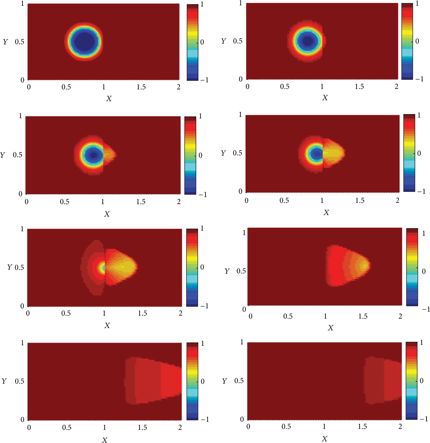
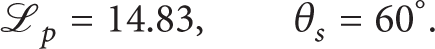
Snapshots of ϕ in free flow region and S _w in porous media region calculated by time step dt = 0.1h are shown in Figure 2. It is clear to see that the two-phase flow transports mainly along the principle direction and the anisotropic property of porous media also has an influence on the velocity and pressure of two-phase flow in the free fluid region in a coupling system. We plot the phase and saturation profile at four points in Figure 3. It is clear that both ϕ and S _w change smoothly.

Figure 2:

Snapshots of ϕ in free flow region and S _w in anisotropic porous media region calculated by time step dt = 0.1h at time t = 0.0040, 0.3240, 0.6440, 0.9640, 1.2840, 1.6040, 1.9240, and 1.9960. Here θ _s = 60° at interface Γ _I and the top and bottom boundaries.

Figure 3:

(a) ϕ on point (0.8, 0.5). (b) ϕ on point (1.0, 0.5) in free flow region. (c) S _w on point (1.0, 0.5) in anisotropic porous media region. (d) S _w on point (1.2, 0.5). It is clear that both phase profile and saturation change smoothly. No oscillation occurs.

To make a comparison, the two-phase flow in coupled free fluid and isotropic porous regions is simulated. We change the absolute permeability and keep other parameters unchanged. The absolute permeability is chosen to be

$\mathbf{K}=\mathrm{1}.$

(62)

Thus, the slip coefficient on the interface becomes

${\mathcal{L}}_p=\mathrm{10}.$

(63)

Snapshots of ϕ in free flow region and S _w in porous media region calculated by time step dt = 0.1h are shown in Figure 4.

Figure 4:

Snapshots of ϕ in free flow region and S _w in porous media region calculated by time step dt = 0.1h at time t = 0.0040, 0.3000, 0.5000, 0.6400, 0.7800, 0.9640, 2.8840, and 4.8040. Here θ _s = 60° at interface Γ _I and the top and bottom boundaries.

4.2. A Layer of Nonwetting Phase Passing through an Interface

A layer of nonwetting phase locating at {[x,y] ∣ 0.75 ≤ x ≤ 1} is put in the free flow region where ϕ⁰ = − 1 inside the layer and ϕ⁰ = 1 outside the layer. The initial saturation S⁰ in the porous media region is set to be S _wc . The time step used is dt = 0.1 × h, where h is the edge length of the triangle elements and h = 1/50. In this example, the dynamic interface intersects with upper and lower boundaries.

The parameters used in the CH-NS equations are listed as follows:

$\begin{array}{c}\mathcal{R}=\mathrm{5},\hspace{1em}\hspace{1em}ϵ=\mathrm{0.02},\hspace{1em}\hspace{1em}\mathcal{B}=\mathrm{12},\\ {\mathcal{V}}_s=\mathrm{50},\hspace{1em}\hspace{1em}{\mathcal{L}}_d=\mathrm{0.05}.\end{array}$

(64)

On the top and bottom boundaries, the slip coefficient and the static contact angle are chosen to be

${\mathcal{L}}_s=\mathrm{0.0038},\hspace{1em}\hspace{1em}{\theta }_s=\mathrm{6}{\mathrm{0}}^{°}.$

(65)

On the interface Γ _I , they are

${\mathcal{L}}_p=\mathrm{14.83},\hspace{1em}\hspace{1em}{\theta }_s=\mathrm{6}{\mathrm{0}}^{\circ }.$

(66)

The parameters used in the Darcy law are listed as follows:

$\begin{array}{c}{\rho }_w=\mathrm{1},\hspace{1em}\hspace{1em}{\rho }_o=\mathrm{1},\hspace{1em}\hspace{1em}\phi =\mathrm{0.2},\hspace{1em}\hspace{1em}{\nu }_w=\mathrm{2},\\ {\nu }_o=\mathrm{2},\hspace{1em}\hspace{1em}{S}_{wc}=\mathrm{0.22},\hspace{1em}\hspace{1em}{S}_{or}=\mathrm{0}.\end{array}$

(67)

The absolute permeability is

$\mathbf{K}=\left(\begin{array}{cc}\mathrm{1.55}& \mathrm{0.78}\\ \mathrm{0.78}& \mathrm{0.65}\end{array}\right).$

(68)

The parameters used for iteration are list as follows:

${\gamma }_f=\mathrm{0.2},\hspace{1em}\hspace{1em}{\gamma }_p=\mathrm{0.2},\hspace{1em}\hspace{1em}{\eta }_f^{\mathrm{0}}=\mathrm{0},\hspace{1em}\hspace{1em}{\eta }_p^{\mathrm{0}}=\mathrm{0}.$

(69)

A parabolic velocity field is put on Γ_in (left boundary), and to avoid the whole system being singular, a pressure is assigned on Γ_out (right boundary).

Snapshots of ϕ in free flow region and S _w in porous media region calculated by time step dt = 0.1h are shown in Figure 5. In this case, the dynamic interface interacts with top and bottom boundaries. The contact angle for the initial condition is 90° and the static contact angle is chosen to be 60° (it is defined as the angle between the contact line and solid wall on the side of phase ϕ = 1). This results in a relatively large slip velocity. We see that the phase propagates faster along the top and bottom boundaries and the two-phase flow transports mainly along the principle direction. We also plot the phase and saturation profile on four points in Figure 6. It is clear that both ϕ and S _w change smoothly. No oscillation happens.

Figure 5:

Snapshots of ϕ in free flow region and S _w in anisotropic porous media region calculated by time step dt = 0.1h at time t = 0.0040, 0.0360, 0.0680, 0.1000, 0.1320, 0.1640, 0.1960, and 0.2200. Here θ _s = 60° at interface Γ _I and the top and bottom boundaries.

Figure 6:

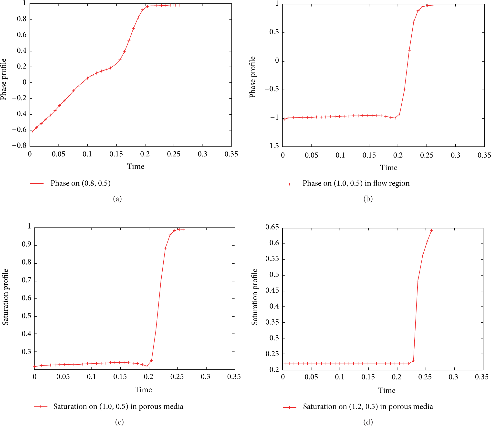
(a) ϕ on point (0.8, 0.5). (b) ϕ on point (1.0, 0.5) in free flow region. (c) S _w on point (1.0, 0.5) in anisotropic porous media region. (d) S _w on point (1.2, 0.5). It is clear that both phase profile and saturation change smoothly. No oscillation happens.

We next change absolute permeability and keep other parameters unchanged. The absolute permeability is chosen to be

$\mathbf{K}=\mathrm{1}.$

(70)

Thus, the slip coefficient on the interface becomes

${\mathcal{L}}_p=\mathrm{10}.$

(71)

Snapshots of ϕ in free flow region and S _w in porous media region calculated by time step dt = 0.1h are shown in Figure 7.

Figure 7:

Snapshots of ϕ in free flow region and S _w in porous media region calculated by time step dt = 0.1h at time t = 0.0040, 0.3000, 0.7800, 0.9640, 1.2040, 1.6040, 2.8840, and 4.8040. Here θ _s = 60° at interface Γ _I and the top and bottom boundaries.

5. Conclusions

In this paper, the two-phase flow crossing the interface between free flow region and anisotropic porous media region is considered. Based on a semi-implicit finite element method for the coupled Cahn-Hilliard and Navier-Stokes system and IMPES method for the two-phase Darcy law, we propose a Robin-Robin domain decomposition method for the coupled system with the generalized Navier interface boundary condition at the interface between the free flow and the porous media regions. Numerical examples show that anisotropic properties of porous medium have a significant effect on streamlines of the flow. As a consequence, the velocity and pressure distribution is quite different for isotopic and anisotropic cases. The numerical methods proposed in this paper have the ability to deal with the coupling domain of free flow region and anisotropic porous media region and the influence of anisotropic properties can be captured by our model of two-phase flow in a coupled domain and corresponding numerical treatment.

Conflict of Interests

The authors declare that there is no conflict of interests regarding the publication of this paper.