Sage Journals: Discover world-class research

Abstract

Micromilling can fabricate miniaturized components using micro-end mill at high rotational speeds. The analysis of machining stability in micromilling plays an important role in characterizing the cutting process, estimating the tool life, and optimizing the process. A numerical analysis and experimental method are presented to investigate the chatter stability in micro-end milling process with variable milling tool geometry. The schematic model of micromilling process is constructed and the calculation formula to predict cutting force and displacements is derived. This is followed by a detailed numerical analysis on micromilling forces between helical ball and square end mills through time domain and frequency domain method and the results are compared. Furthermore, a detailed time domain simulation for micro end milling with straight teeth and helical teeth end mill is conducted based on the machine-tool system frequency response function obtained through modal experiment. The forces and displacements are predicted and the simulation result between variable cutter geometry is deeply compared. The simulation results have important significance for the actual milling process.

1. Introduction

There is a strong demand from various industries for miniature devices and components with complex microscale features fabricated on a variety of materials. Micro-end milling can overcome the limitations of semiconductor based processing techniques by utilizing miniature tools to make complex 3D parts from different engineering materials with no need for expensive masks [1 –4]. Due to the fragile nature of the miniature tools, even minute vibration in micro-end milling can lead to part failures. Therefore, how to set cutting conditions is very important. When cutting conditions are not appropriate, tools are easily fractured, which wastes time and money [2, 5, 6]. In addition, in micro-end milling, cutting forces, and the tool tip displacements play an important role in the determination of the characteristics of cutting processes like tool wear and surface texture, the establishment of cutting plans, and the setting of cutting conditions. It is very important to study the dynamics of cutting forces and displacements in any machining process for proper planning and control of machining process and for the optimization of the cutting conditions to minimize production costs and times [7 –9].

Usually, the milling tool has two different types, square and ball cutter; and the flat cutter has two different edge geometries, straight teeth and helical teeth. As for us, milling tool with straight cutting teeth is relatively simple for the cutting width is equal to the axial cutting depth. However, if the cutter teeth are helical, the portion of each tooth that is engaged in the cut varies as the tool rotates. The changing deflection of the tool is imprinted on the machined surface parallel to the tools’ axis of rotation. It is difficult to include this complexity in the analytical formulations, but relatively straightforward to include in the time domain and frequency domain simulation. The analytical stability lobe diagrams provide a global picture of the stability behavior but do not provide information regarding the local cutting force or tool vibrations [10 –12]. The time domain simulation, on the other hand, gives this local force and vibration information for the selected cutting conditions. The simulation again applies numerical integration to solve the time delayed differential equations of motion and includes the nonlinearity that occurs if the tooth leaves the cut [13].

For this and many other reasons, time domain and frequency domain simulation is a better representation of the cutting process than either of the methods described earlier. In all engineering fields, it is that increased accuracy is computationally more intensive. A method combining time domain and frequency domain analysis is chosen in this paper to investigate the micromilling stability with variable tool geometry.

2. Dynamic Model

Micro-end milling is described as a two-degree-of-freedom system, as shown in reference [14] by our research group. For this simulation, we will neglect the possibility that the current surface may depend on more than the prior and current tooth vibrations.

2.1. Cutting Force Calculation

As the cutting force can be expressed by the chip thickness variation with cutter angle, the number of teeth simultaneously engaged in the cut at any instant. The cutting force on any cutting edge can be expressed as a function of the chip area and specific cutting force:

F = k_{s} b h,

(1)

where F_c is cutting force, k_s is specific cutting force, b is chip width, and h is chip thickness. The normal, tangential, and axial force components can be written as the following:

\begin{matrix} F_{n} = k_{n} b h \\ F_{t} = k_{t} b h \\ F_{a} = k_{a} b h, \end{matrix}

(2)

where F_n, F_t, and F_a are normal, tangential, and axial cutting force, k_t is the cutting coefficient in the tangential direction, k_n is the cutting coefficient in the normal direction, and k_a is the cutting coefficient in the axial direction. Once the chip thickness and width are determined, the cutting force components in the tangential, normal, and axial directions are determined for each axial slice.

To describe these forces analytically, we must project the normal, tangential, and axial components into the x, y, and z coordinate directions. When the ball surface normal direction angle is set as 90 deg, the x and y force projections are now identical to the helical square end mill simulation and the z component is equal to the axial force. The formula is expressed as the following:

(\begin{pmatrix} F_{x} \\ F_{y} \\ F_{z} \end{pmatrix}) = [\begin{bmatrix} \cos ϕ & \sin ϕ & 0 \\ \sin ϕ & - \cos ϕ & 0 \\ 0 & 0 & - 1 \end{bmatrix}] (\begin{pmatrix} F_{t} \\ F_{n} \\ F_{a} \end{pmatrix}),

(3)

where ϕ is the instantaneous cutter angle and F_x, F_y, and F_z are the cutting force in x, y, and z direction, respectively. The resultant force F is calculated using

F^{2} = F_{x}^{2} + F_{y}^{2} + F_{z}^{2} .

(4)

2.2. Displacement Calculation

Considering a single degree of freedom in the x and y directions, the equation of motion can be described as

\begin{matrix} M_{x} \ddot{x} + C_{x} \dot{x} + K_{x} x = F_{x} \\ M_{y} \ddot{y} + C_{y} \dot{y} + K_{y} y = F_{y}, \end{matrix}

(5)

where M_x, C_x, and K_x are the effective mass, damping coefficient, and stiffness; the same formulation can be applied to y direction as well. The new velocities and positions are then determined by numerical integration. The new velocities are then applied to determine the new displacements. Multiple degrees of freedom in each direction can be accommodated by summing the individual modal contributions.

2.3. Simulation Implementation

The milling simulation completes three basic activities at each time step. First, the cutter is rotated by dϕ by adding one to each entry in the teeth vector. Second, within a loop that sums over all the cutter teeth, it is first verified that the tooth in question is bounded by the start and exit cut angles. If so, the chip thickness is determined and the cutting force is calculated. If not, the force is set to zero. Third, the displacement is determined by numerical integration.

3. Results and Discussions

3.1. Comparison of Cutting Forces between Ball and Square End Mills

The cutting forces produced by helical square and ball end mills are compared in order to investigate the influence of variable tool geometry on cutting forces. In this simulation experiment, a 35% radial immersion (a radial immersion ordinarily used) down milling cut is considered. There are two identical modes in both the x and y directions obtained through modal testing method, and the experimental device is shown in Figure 1. These are expressed in modal coordinates as f_n1 = 1000 Hz, k₁ = 2.6 × 10⁶ N/m, and ζ₁ = 0.03; and f_n2 = 1200 Hz, k₂ = 1.8 × 10⁶ N/m, and ζ₂ = 0.02. An aluminum alloy is machined with both four tooth end mill whose diameter is 1 mm using a feed per tooth of 0.5 μm/tooth. For a specific force value of K_s = 950 N/mm² and force angle of 60 deg, the corresponding cutting force coefficients are k_t = 1510 N/mm² and k_n = 1264 N/mm². The axial coefficient, k_a, is taken to be equal to k_n. f_n is natural frequency, k is stiffness, and ζ is damping ratio.

Figure 1:

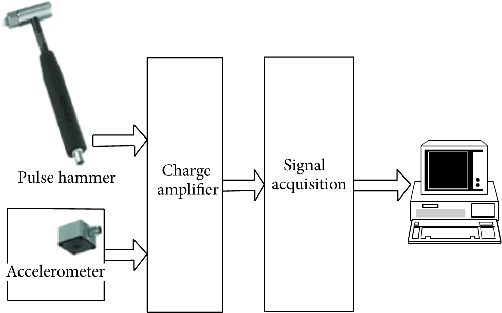
Modal test setup.

The axial cutting depth is 0.4 mm, the helix angle is 45 deg, and spindle speed used is 15000 rpm in these simulations. For the simulations, 2000 steps per revolution is used and the results for the cutting forces in the x, y, and z directions under these machining conditions are displayed in Figure 2 through Figure 5, respectively.

Figure 2:

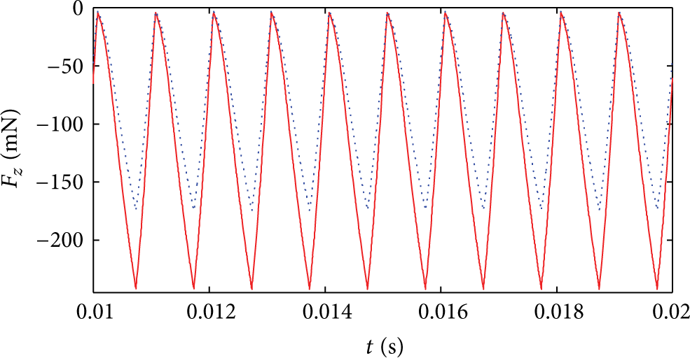
Comparison of x direction cutting force for ball (solid line) and square (dotted line) helical end mills.

As shown in Figures 2, 3 and 4, differences are observed in all three directions. This is due to the variation in the ball surface normal angle and the corresponding projections of the normal and axial components. Naturally, the resultant force is the same for both end mills according to Figure 5. Actually, which end mill to choose depends on the specific machining conditions.

Figure 3:

Comparison of y direction cutting force for ball (solid line) and square (dotted line) helical end mills.

Figure 4:

Comparison of z direction cutting force for ball (solid line) and square (dotted line) helical end mills.

Figure 5:

Comparison of resultant cutting force for ball (solid line) and square (dotted line) helical end mills.

3.2. Comparison of Stability Simulation Result between Time Domain and Frequency Domain in Ball Micromilling

Symmetric dynamics with 5% radial immersion (small radial immersion) up milling cut is considered in this simulation experiment, f = 1500 Hz, k = 2.2 × 10⁶ N/m, and $ζ_{}$ = 0.012. The workpiece is aluminum alloy machined with four tooth end mill, 1 mm diameter with 45 deg helix angle and using a feed per tooth of 0.4 μm/tooth. The cutting force coefficients are k_t = 1250 N/mm² and k_n = 1384 N/mm². The simulation result obtained is displayed in Figure 6.

Figure 6:

The time domain simulation result is compared to frequency domain solution stability.

The stability limit obtained using the frequency domain solution is shown in Figure 6 as a solid line. The results of time domain simulations are identified by dot (stable); box (Hopf bifurcation); and triangle (flip bifurcation) [15, 16]. It can be seen from Figure 6 that a narrow band of increased stability is between 45000 rpm and 46000 rpm. This is accompanied by the spindle speed range from 47000 rpm to 50000 rpm which exhibits flip bifurcation behavior.

3.3. Stability Analysis at Low Radial Immersion

Two case points are selected for further study of stability behavior. The once-per-revolution sampled data is expressed as “+” symbol in all three simulations.

The simulation results of case point (n = 46000 rpm and a_lim = 0.8 mm) from Figure 6 are shown in Figures 7 and 8, which demonstrates the time displacements and the x versus y plot, respectively.

Figure 7:

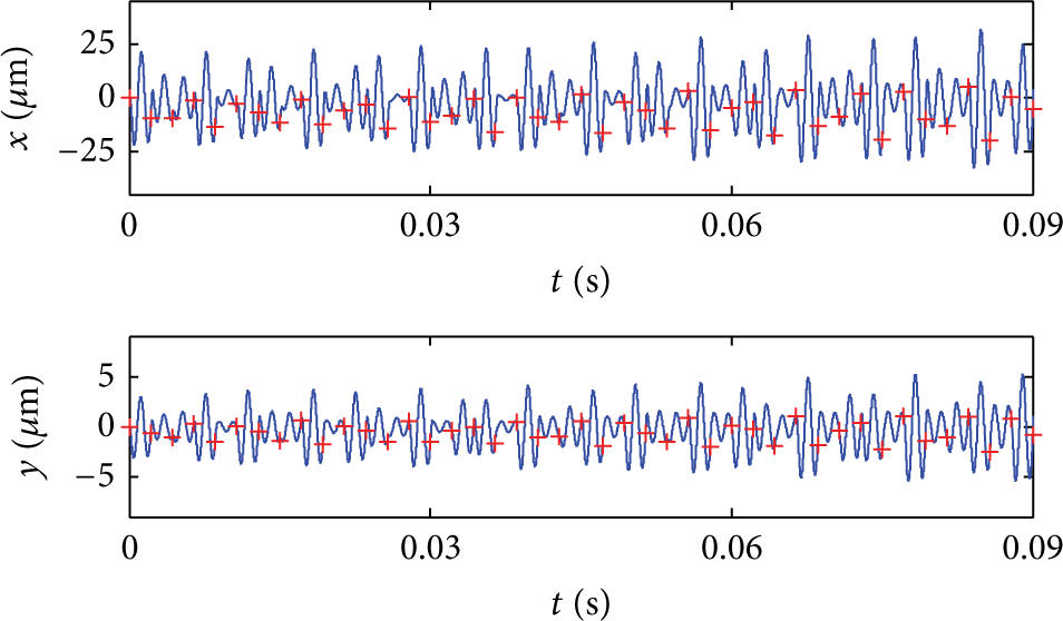
Simulation results for x and y direction displacements (n = 46000 rpm and a_lim = 0.8 mm).

Figure 8:

Plot of x versus y direction displacements (n = 46000 rpm and a_lim = 0.8 mm).

The traditional Hopf instability can be seen in this simulation because the once-per-revolution sampled data appears as an elliptical distribution for Hopf instability.

Furthermore, the simulation results of case point (n = 50000 rpm and a_lim = 0.7 mm) are shown in Figures 9 and 10.

Figure 9:

Simulation results for x and y direction displacements (n = 50000 rpm and a_lim = 0.7 mm).

Figure 10:

Plot of x versus y direction displacements (n = 50000 rpm and a_lim = 0.7 mm).

As expected, Figures 9 and 10 display repetitive behavior from one revolution to the next. A stable cut is observed in this simulation. For practical machining applications, the radial depth of cut is needed to consider. When the radial depth of cut is low, additional stable zones appear that “split” the higher radial depth stability lobes.

3.4. Time Domain Simulation by Square End Mill with Straight Teeth

Because we have assumed straight teeth, we will ignore vibrations in the z direction. The x and y direction dynamics of machining system are symmetric with f_n = 600 Hz, k = 2.8 × 10⁶ N/m, and ζ = 0.04. An aluminum alloy is machined with a four tooth square end mill and the cutting force coefficients are k_t = 1780 N/mm², k_n = 1268 N/mm², and K_s = 1426 N/mm². For the slotting cut, the start angle is 0 and exit angle is 180 deg. f_n is natural frequency, k is stiffness, and ζ is damping ratio.

Two different cases are considered: (1) n = 15000 rpm and b = 0.3 mm; (2) n = 15000 rpm and b = 0.5 mm. Figures 11 and 12 show the x and y direction forces and displacements, respectively, for case 1.

Figure 11:

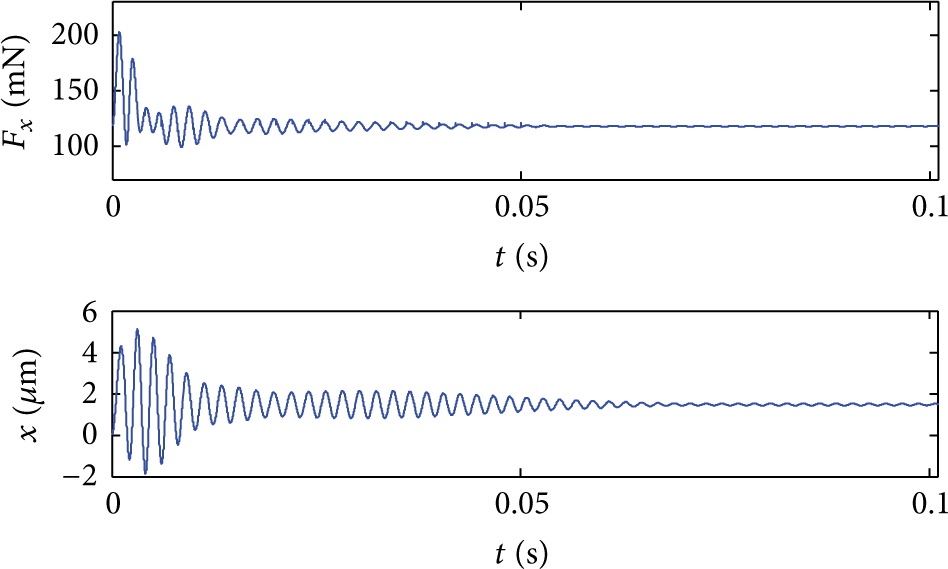
Simulation results for x direction force and displacement (n = 15000 rpm and b = 0.3 mm).

Figure 12:

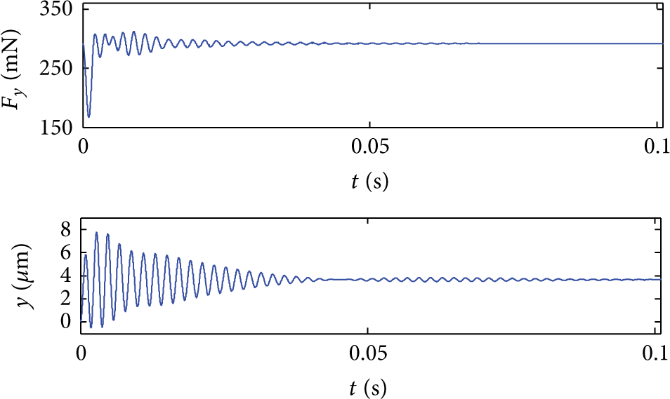
Simulation results for y direction force and displacement (n = 15000 rpm and b = 0.3 mm).

It is seen that, once the initial transients attenuate after approximately 0.06 s, the expected constant force for a four-tooth cutter in a slotting cut is obtained. Case 1 provides stable operating conditions.

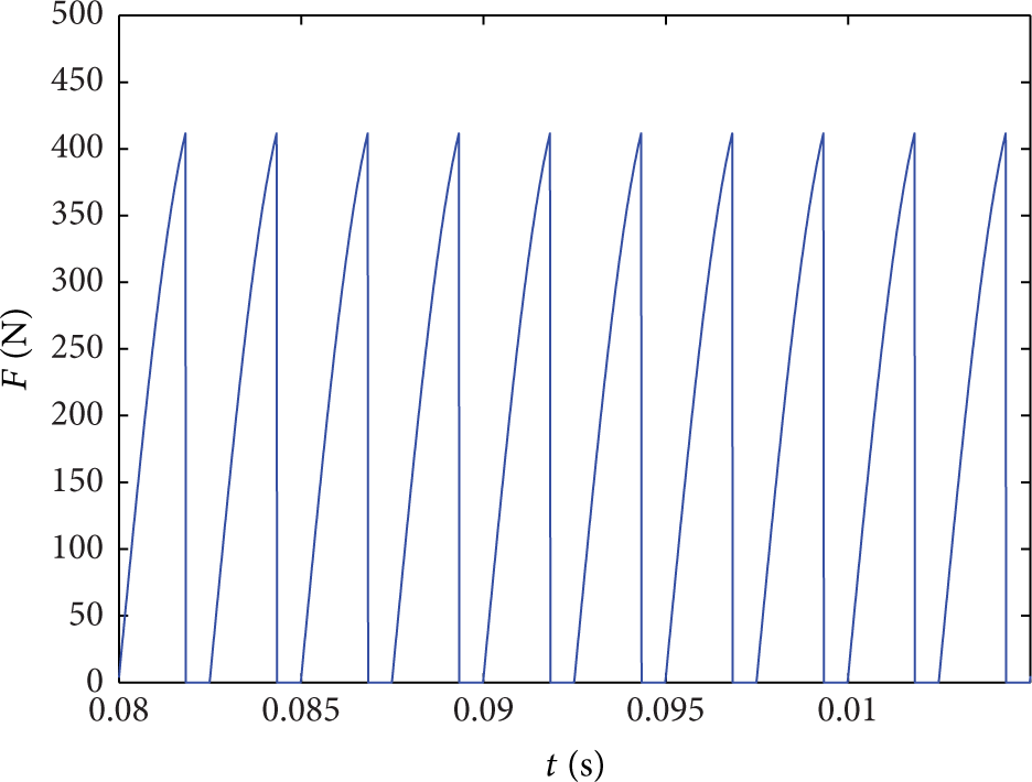
Figures 13 and 14 display the x and y direction results for case 2.

Figure 13:

Simulation results for x direction force and displacement (n = 15000 rpm and b = 0.5 mm).

Figure 14:

Simulation results for y direction force and displacement (n = 15000 rpm and b = 0.5 mm).

It can be seen from Figures 13 and 14 that the maximum forces are up to 1000 mN and the tool tip displacement increases to about 50 μm instantaneously. So chatter is observed which may result in a poor surface finish and reduce the longevity of the tool in the actual milling process. We need further study to determine chatter-free conditions in micromilling operation.

3.5. Milling Time Domain Simulation by Square End Mill with Helical Teeth

While the simulation described above is capable of predicting forces and displacement in milling process, the assumption of straight cutter teeth is rarely applicable in practice. The cutting edges are typically inclined at the helix angle β, so that the chip to be removed is spread over an increased length and the cutting edge pressure is reduced. The result of the helical cutting edge geometry is that the full length of the cutting edge does not enter (or exit) the cut at the same instant. Instead, there is an increasing delay of the cut entry (and exit) when moving from the free end of the cutter toward the spindle.

Strictly speaking, due to the helical geometry, we should also consider the axial (z direction) forces and potential deflections. However, for most end milling applications, the z direction dynamic stiffness is much higher than the x or y direction stiffness values, so it is common to consider the z direction to be rigid.

3.6. Comparison of Forces between Straight and Helical Teeth

In this simulation experiment, we compare the cutting forces produced by straight and helical teeth with all other conditions being equal. We also model a 35% radial immersion up milling cut. There are two identical modes in both the x and y directions obtained through modal testing method [14]. These are expressed in modal coordinates as f_n1 = 1000 Hz, k_q1 = 2.6 × 10⁶ N/m, and ζ₁ = 0.03; and f_n2 = 1200 Hz, k_q2 = 1.8 × 10⁶ N/m, and ζ₂ = 0.02. The workpiece material is an aluminum alloy and it is machined with a four-tooth, 16 mm in diameter square end mill using a feed per tooth of 0.6 μm/tooth. For a specific force value of K_s = 950 N/mm² and force angle of 60 deg, the corresponding cutting force coefficients are k_t = 1510 N/mm² and k_n = 1264 N/mm². Figures 15 and 16 show the resultant cutting forces (in the x-y plane) for a small time portion of the simulation result with b = 0.5 mm and helix angles of zero and 45 deg, respectively.

Figure 15:

Resultant cutting force versus time for zero helix angle end mill (n = 15000 rpm and b = 0.5 mm).

Figure 16:

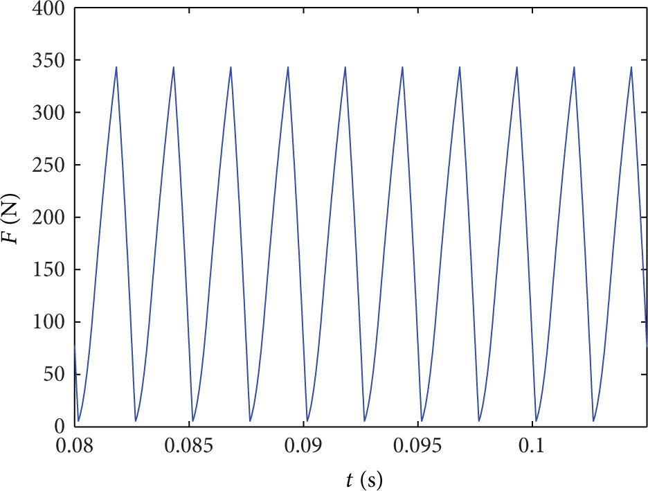
Resultant cutting force versus time for 45 deg helix angle end mill (n = 15000 rpm and b = 0.5 mm).

A comparison of the two figures shows clear differences. First, the maximum cutter force is lower for the helical teeth end mill. Second, the force grows to its maximum value and then abruptly drops to zero at the cut exit angle for the straight tooth end mill. For the helical teeth cutter, on the other hand, the force grows and then decreases in a more saw tooth pattern and does not quite reach zero.

4. Conclusions

This study presented a numerical analysis method for predicting the force and displacement on the developed dynamics model of micro-end milling process. It took into account the dynamic cutting thickness, cutting force and tool tip displacement, and constructed the relevant equations.

The cutting forces between ball and square end mills are compared by time domain simulation. In addition, the stability lobe of ball micromilling at low radial immersion is researched detailed through time domain and frequency domain method. Furthermore, the time displacements and the x versus y plots are obtained and the simulation result between variable stability cases is compared.

In addition, this study performed a detailed time domain simulation for micro-end milling with straight teeth and helical teeth end mill to predict the forces and displacements, and the result between variable cutter geometries is deeply analyzed.

Conflict of Interests

The authors declare that there is no conflict of interests regarding the publication of this paper.

Footnotes

Acknowledgments

This project is supported by National Natural Science Foundation of China (Grant no. 51305286), Jiangsu Natural Science Foundation (BK2011314), and Suzhou Science and Technology Projects (SYG201244), and it is also sponsored by Qing Lan Project of Jiangsu Province.

References

Huang

C. Y.

and Wang

J. J. J.

, “Mechanistic modeling of process damping in peripheral milling,” Journal of Manufacturing Science and Engineering, vol. 129, no. 1, pp. 12–20, 2007.

Quintana

and Ciurana

, “Chatter in machining processes: a review,” International Journal of Machine Tools and Manufacture, vol. 51, no. 5, pp. 363–376, 2011.

Dornfeld

Min

, and Takeuchi

, “Recent advances in mechanical micromachining,” Annals of the CIRP, vol. 55, no. 2, pp. 745–768, 2006.

Afazov

S. M.

Zdebski

Ratchev

S. M.

Segal

, and Liu

, “Effects of micro-milling conditions on the cutting forces and process stability,” Journal of Materials Processing Technology, vol. 213, no. 5, pp. 671–684, 2013.

Vogler

M. P.

Kapoor

S. G.

, and deVor

R. E.

, “On the modeling and analysis of machining performance in micro-endmilling, part II: cutting force prediction,” Journal of Manufacturing Science and Engineering, Transactions of the ASME, vol. 126, no. 4, pp. 695–705, 2004.

Davies

M. A.

Pratt

J. R.

Dutterer

, and Burns

T. J.

, “Stability prediction for low radial immersion milling,” Journal of Manufacturing Science and Engineering, vol. 124, no. 2, pp. 217–225, 2002.

Davies

M. A.

Pratt

J. R.

Dutterer

B. S.

, and Burns

T. J.

, “Stability of low radial immersion milling,” Annals of the CIRP, vol. 49, no. 1, pp. 37–40, 2000.

Chae

, Development and Analysis of the Precision Micro End Milling System, University of Calgary, 2006.

Park

S. S.

and Malekian

, “Mechanistic modeling and accurate measurement of micro end milling forces,” CIRP Annals - Manufacturing Technology, vol. 58, no. 1, pp. 49–52, 2009.

10.

Chae

Park

S. S.

, and Freiheit

, “Investigation of micro-cutting operations,” International Journal of Machine Tools and Manufacture, vol. 46, no. 3–4, pp. 313–332, 2006.

11.

Altintas

Eynian

, and Onozuka

, “Identification of dynamic cutting force coefficients and chatter stability with process damping,” CIRP Annals: Manufacturing Technology, vol. 57, no. 1, pp. 371–374, 2008.

12.

Salahshoor

and Ahmadian

, “Continuous model for analytical prediction of chatter in milling,” International Journal of Machine Tools and Manufacture, vol. 49, no. 14, pp. 1136–1143, 2009.

13.

Altintas

Stepan

Merdol

, and Dombovari

, “Chatter stability of milling in frequency and discrete time domain,” CIRP Journal of Manufacturing Science and Technology, vol. 1, no. 1, pp. 35–44, 2008.

14.

Cao

and Li

, “Research on regenerative chatter in micro milling process,” Hydromechatronics Engineering, vol. 40, pp. 17–20, 2012.

15.

Campomanes

M. L.

and Altintas

, “An improved time domain simulation for dynamic milling at small radial immersions,” Journal of Manufacturing Science and Engineering, vol. 125, no. 3, pp. 416–422, 2003.

16.