Sage Journals: Discover world-class research

Abstract

The present paper provides a first step to a new approach to the theory of gearing, which uses modern differential geometry in order to ensure a strict and coordinate-independent formulation. Here, we are mainly concerned with a basic equation, namely, the equation of meshing, of two rotating surfaces in mesh. Since we are able to solve this equation by the time parameter, we derive parameterizations of the mating pinion from a bevel gear as well as a parameterization for gears produced by special machine tools.

1. Introduction

The definition of the tooth surface of a spiral bevel gear usually uses the settings of a special machine tool. In contrast, one needs an explicit description of the surface in Euclidean coordinates to generate such a gear on a CNC-machine. This seems to be complicated, since the computation of the envelope of a family of surfaces is involved in this process. Classical attempts like those presented in Litvin and Fuentes [1], as well as more recently approaches proposed by Dooner [2], rely on the introduction of several coordinate systems that are fixed to several parts of the machine tool. A first step towards a coordinate-free description can be found in di Puccio et al. [3]: the authors use the linear algebra of rotations. Nevertheless, if the rotations have nonintersecting axes, then this approach is not fully satisfactory, too.

The present paper provides an introduction to the theory of gearing within both mathematical and mechanical strict setting of Euclidean geometry. We use the theory of the Euclidean motion group, which is well known in mechanics, especially in control theory; see Bullo and Lewis [4]. The main advantages of this approach are as follows.

A coordinate-free description leads to expressions that are meaningful in both a mechanical and a mathematical sense.

For computations, one has to deal with one coordinate frame only, which one can choose freely.

The derived equations are very compact. Moreover, they lead to a clear understanding of the theory.

The approach provides an explicit solution of the equation of meshing in a very general situation.

By applying the latter result, one obtains explicit formulas for gear surfaces generated by special machine tools as well as for the mating pinion of a given bevel gear. Similar results can be obtained easily for spur gears.

In several subsequent papers, we will extend the theory to the kinematics, dynamics, and the geometry of gear drives. Most recently, the results have been applied to the remanufacturing of a pinion of a bevel gear drive; see [5] for the details.

The paper is organized as follows. First, we give a short review on motions of the Euclidean 3-space. In particular, we will need Rodrigues’ formulas (4) and (7). The third section is devoted to the equation of meshing: we consider surfaces Γ₁,Γ₂ in mesh, which are given by parameterizations in Euclidean coordinates. Viewed from a coordinate frame fixed to Γ₂, the surface Γ₁ performs a rigid motion and, thus, yields a family of surfaces. Then, Γ₂ turns out to be the envelope of this family. This fact leads to a version of the (well-known) equation of meshing (17) which has a strict mechanical interpretation in our setting. In fact, we are able to solve the equation of meshing by the time parameter, and, hence, obtain an explicit parameterization (31) of Γ₂. The last two sections are devoted to applications: first, we derive the parameterization of the mating pinion of an existing bevel gear. We remark that we may derive similar results for spur gears in the very same way. Finally, we investigate parameterizations of gears produced by face hobbing machines in a quite general context and apply the obtained results to spiral bevel gears.

2. Motions of the 3-Space

We will distinguish between points and vectors of the Euclidean 3-space E₃ by adding a fourth component; that is, we will write $P = (\begin{smallmatrix} p \\ 1 \end{smallmatrix})$ for the point p ∈ R₃ and $v = (\begin{smallmatrix} v \\ 0 \end{smallmatrix})$ for the vector v ∈ R₃. Note that one may take a linear combination t₁v₁ + ⋯ + t_nv_n of vectors v ₁,…, v _n as usual. Moreover, the sum P + v of a point P and a vector v yields a point, while the difference P − Q of two points P,Q is a vector, as expected. We point out that the sum of points is not defined (as the fourth component would be different from 1), but one can take affine combinations tP + (1 − t)Q. Finally, we agree on the following notation: for vectors $v_{j} = (\begin{smallmatrix} v_{j} \\ 0 \end{smallmatrix})$ , we put 〈v₁ ∣ v₂〉 = 〈 v ₁ ∣ v ₂〉 (where 〈· ∣ ·〉 denotes the usual scalar product),det⁡ ⁡(v₁,v₂,v₃) = det⁡⁡ ( v ₁, v ₂, v ₃), and v₁∧v₂ = v ₁∧ v ₂ (where ∧ denotes the cross product).

An advantage of the notation introduced above is a very natural setting for affine maps α( p ) = R· p + u , where R is a 3 × 3-matrix and u ∈ R₃ denotes the translation part. Recall that the image of a vector v ∈ R₃ is given by α( v ) = R · v . These equations can be written as

(\begin{pmatrix} R & u \\ 0 & 1 \end{pmatrix}) \cdot (\begin{pmatrix} p \\ 1 \end{pmatrix}) = (\begin{pmatrix} R \cdot p + u \\ 1 \end{pmatrix}), (\begin{pmatrix} R & u \\ 0 & 1 \end{pmatrix}) \cdot (\begin{pmatrix} v \\ 0 \end{pmatrix}) = (\begin{pmatrix} R \cdot v \\ 0 \end{pmatrix});

(1)

that is, the affine map α is represented by the 4 × 4-matrix $A = (\begin{smallmatrix} R & u \\ 0 & 1 \end{smallmatrix})$ . An easy computation shows that the composition of affine maps is related to the multiplication of the corresponding matrices.

We are mainly interested in motions of the Euclidean space, that is, in those affine maps, which does not change the distance or the orientation. Recall that an affine map is a motion if and only if its linear part R is a rotation; that is, R fulfils R^T·R = I₃ and det⁡⁡R = 1, where the superscript T refers to the transpose of a matrix and I_k denotes a k × k-unit matrix. If we let SO(3) and SE(3) be the sets of all linear rotations and of all motions, respectively, then SO(3) and SE(3) are the so-called Lie groups, that is, groups with an additional structure of a smooth manifold such that the group operations become smooth maps. We will not go into details here; the reader will find an introduction (and all results cited below as well) in Bullo and Lewis [4].

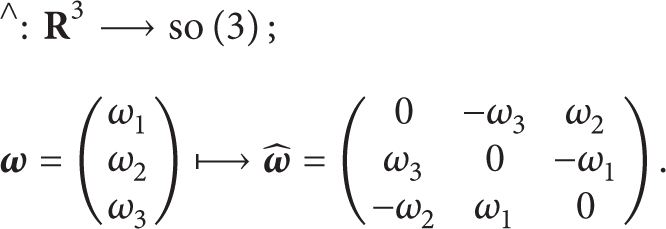
The Lie algebraso(3) of SO(3) is the vector space of skew-symmetric 3 × 3-matrices. The following isomorphism of vector spaces will be used repeatedly:

\begin{array}{l} {}^{\land}: R^{3} ⟶ so (3); \\ ω = (\begin{pmatrix} ω_{1} \\ ω_{2} \\ ω_{3} \end{pmatrix}) ⟼ \hat{ω} = (\begin{pmatrix} 0 & - ω_{3} & ω_{2} \\ ω_{3} & 0 & - ω_{1} \\ - ω_{2} & ω_{1} & 0 \end{pmatrix}) . \end{array}

(2)

The so-called hat-operator “∧,” whose inverse will be denoted by the superscript “∨,” has the following properties:

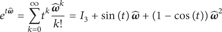
\begin{matrix} \hat{ω} \cdot v = ω \land v \forall ω, v \in R^{3} . \\ {(ω \land μ)}^{\land} = [\hat{ω}, \hat{μ}] ≔ \hat{ω} \cdot \hat{μ} - \hat{μ} \cdot \hat{ω} \forall ω, μ \in R^{3} . \\ R \cdot \hat{ω} \cdot R^{- 1} = {(R ω)}^{\land} \forall ω \in R^{3}, R \in SO (3) . \end{matrix}

(3)

As usual, Lie group and Lie algebra are connected by the exponential map, which has a particular geometrical meaning in the context of rotations: if ω ∈ R₃ has length $| ω | = 1$ and if t is a real number, then the exponential

e^{t \hat{ω}} = \sum_{k = 0}^{\infty} t^{k} \frac{{\hat{ω}}^{k}}{k!} = I_{3} + \sin (t) \hat{ω} + (1 - \cos (t)) {\hat{ω}}^{2}

(4)

is a rotation with axis R·ω and angle t. We will refer to (4) as the formula of Rodrigues. Note that

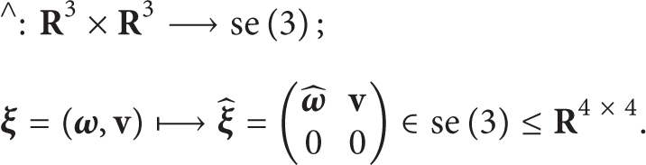
\begin{array}{l} \frac{d}{d t} e^{t \hat{ω}} v = \hat{ω} e^{t \hat{ω}} v = ω \land (e^{t \hat{ω}} v) \\ = e^{t \hat{ω}} \hat{ω} v = e^{t \hat{ω}} (ω \land v) \forall v \in R . \end{array}

(5)

There is also a hat-operator for the Lie algebra se(3) of SE(3); namely,

\begin{matrix} {}^{\land}: R^{3} \times R^{3} ⟶ se (3); \\ ξ = (ω, v) ⟼ \hat{ξ} = (\begin{pmatrix} \hat{ω} & v \\ 0 & 0 \end{pmatrix}) \in se (3) \leq R^{4 \times 4} . \end{matrix}

(6)

In the sequel we will identify R₃ and so(3) as well as R₃ × R₃ and se(3) with respect to the hat-operators given in (2) and (6), respectively.

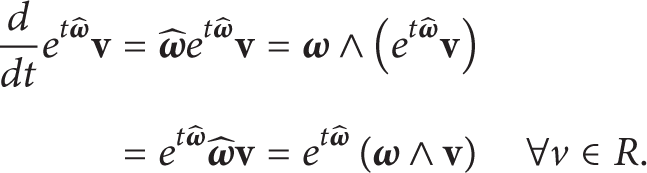
Rodrigues’ formula (4) can be extended to the exponential function se(3) → SE(3) of the Euclidean motion group (cp. [4, 5.1.3]). For the case of rotation, one obtains the following results: consider an element ξ = (ω,v) ∈ se(3) = R₃ × R₃. Then $e^{t \overset{⁁}{ξ}}$ is a rotation for every t if and only if ω≠0 and 〈ω ∣ v 〉 = 0. If, in addition, |ω| = 1, then the exponential of $t \overset{⁁}{ξ}$ (which is given by the usual power series) is given by

e^{t \hat{ξ}} = (\begin{pmatrix} e^{t \hat{ω}} & \sin (t) v + (1 - \cos (t)) \hat{ω} v \\ 0 & 1 \end{pmatrix}) .

(7)

The map $e^{t \overset{⁁}{ξ}}$ defined by (7) is a rotation with axis ω ∧ v + R · ω and angle t. Notice that v = − ω∧ q holds for every point $Q = {(q, 1)}^{T}$ of the axis of the rotation. Moreover, analogous to (5), we obtain for ξ ∈ se(3) a point P and a vector v that

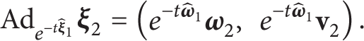
\frac{d}{d t} e^{t \hat{ξ}} \cdot P = e^{t \hat{ξ}} \hat{ξ} P = \hat{ξ} e^{t \hat{ξ}} P, \frac{d}{d t} e^{t \hat{ξ}} \cdot v = e^{t \hat{ξ}} \hat{ξ} v = \hat{ξ} e^{t \hat{ξ}} v .

(8)

Every motion A ∈ SE(3) induces a bijective linear map Ad(A) of the Lie algebra se(3) by putting $Ad (A) (\overset{⁁}{ξ}) = A \overset{⁁}{ξ} A^{- 1}$ . We may also write $Ad (A) (\overset{⁁}{ξ}) = {(A d_{A} \cdot ξ)}^{\land}$ with respect to the identification of se(3) and R₃ × R₃, where Ad_A is the 6 × 6-matrix:

{Ad}_{A} = (\begin{pmatrix} R & 0 \\ \hat{w} R & R \end{pmatrix}) for A = (\begin{pmatrix} R & w \\ 0 & 1 \end{pmatrix}) .

(9)

The function Ad is commonly called the adjoint operator of the Lie group SE(3). The derivate

{\frac{d}{d t} |}_{t = t_{0}} Ad (e^{t \hat{ξ}}) (\hat{μ}) = Ad (e^{t_{0} \hat{ξ}}) (\hat{ξ} \cdot \hat{μ} - \hat{μ} \cdot \hat{ξ})

(10)

directly leads to the adjoint operator ${ad}_{ξ} (μ) = [ξ, μ] = {(\overset{⁁}{ξ} \cdot \overset{⁁}{μ} - \overset{⁁}{μ} \cdot \overset{⁁}{ξ})}^{\lor}$ of the Lie algebra se(3).

Finally, we agree on the notion of a coordinate frame of the Euclidean space to be a quadruple (O,u,v,w) that consisted of a point O (the origin of the frame) and a right-handed orthonormal system (u,v,w) of vectors.

3. The Envelope of a Certain Family of Surfaces

We investigate a quite general situation in this section: we consider two surfaces Γ₁ and Γ₂ in the Euclidean 3-space E₃ given by regular parameterizations:

Γ_{j} : (r, s) ⟼ G_{j} (r, s) = (\begin{pmatrix} g_{j} (r, s) \\ 1 \end{pmatrix}); j = 1,2 .

(11)

We require that Γ₁ is at least C² and that Γ₂ is at least C¹. Notice that the vector

n_{j} (r, s) = (\begin{pmatrix} n_{j} (r, s) \\ 0 \end{pmatrix}) = \frac{\partial G_{j}}{\partial r} \land \frac{\partial G_{j}}{\partial s} = (\begin{pmatrix} \frac{\partial g_{j}}{\partial r} \land \frac{\partial g_{j}}{\partial s} \\ 0 \end{pmatrix}) \neq 0

(12)

is parallel to the normal of Γ_j at the point G_j(r,s).

Let each of the two surfaces perform a rotation of constant angular velocity around a fixed axis. These rotations are given by $e^{t {\overset{⁁}{ξ}}_{1}}$ and $e^{μ t {\overset{⁁}{ξ}}_{2}}$ , respectively, where ξ_j = (ω_j, v _j) ∈ se(3) satisfies |ω_j| = 1 and 〈ω_j ∣ v _j〉 = 0 and μ denotes the signed ratio of angular velocities. We require that μω₂ − ω₁ does not vanish. The angle t of the first rotation will be regarded as the time parameter in the sequel.

One may consider $e^{t {\overset{⁁}{ξ}}_{1}}$ and $e^{μ t {\overset{⁁}{ξ}}_{2}}$ as transformation matrices from a given spatial frame Σ to (moving) body frames B₁, B₂ which are rigidly connected to the surfaces Γ₁ and Γ₂, respectively. Taking an appropriate offset, we may achieve that all three frames coincide at the instant t = 0. In this picture, G_j(r,s) describes the surface Γ_j with respect to the body frame B_j, while $e^{t_{0} {\overset{⁁}{ξ}}_{1}} G_{1} (r, s)$ and $e^{μ t_{0} {\overset{⁁}{ξ}}_{2}} G_{2} (r, s)$ are the parameterization of Γ₁ and Γ₂, respectively, at the instant t = t₀ with respect to the spatial frame Σ. In the sequel, most of the computations will be done in the coordinate frame B ₂ of the second surface Γ₂.

We assume that for each parameter (r,s) there exists an instant t = t(r,s) at which the points G₁(r,s) and G₂(r,s) are in contact. This implies that $e^{t {\overset{⁁}{ξ}}_{1}} G_{1} (r, s) = e^{μ t {\overset{⁁}{ξ}}_{2}} G_{2} (r, s)$ or, equivalently, that

G_{2} (r, s) = e^{- μ t {\hat{ξ}}_{2}} e^{t {\hat{ξ}}_{1}} G_{1} (r, s) .

(13)

Here, $R (t) = e^{- μ t {\overset{⁁}{ξ}}_{2}} e^{t {\overset{⁁}{ξ}}_{1}} \in SE (3)$ describes the motion of the surface Γ₁ with respect to the body frame B ₂ which is rigidly attached to Γ₂. Moreover, we require that the two surfaces share a common normal at their points of contact. As usual, this implies that Γ₂ is the envelope of the family of surfaces given by the C²-function:

F (r, s, t) = e^{- μ t {\hat{ξ}}_{2}} e^{t {\hat{ξ}}_{1}} G_{1} (r, s) .

(14)

We refer the reader to Zalgaller [6] for a detailed discussion of envelopes. In particular, we obtain the following necessary condition, which is commonly called the equation of meshing: if F(r₀,s₀,t₀) is a point of the envelope, then

\begin{array}{l} 0 = \det (\begin{pmatrix} {\frac{\partial F}{\partial r} |}_{(r_{0}, s_{0}, t_{0})}, {\frac{\partial F}{\partial s} |}_{(r_{0}, s_{0}, t_{0})}, {\frac{\partial F}{\partial t} |}_{{(r}_{0}, s_{0}, t_{0})} \end{pmatrix}), \\ = 〈 {\frac{\partial F}{\partial r} |}_{(r_{0}, s_{0}, t_{0})} \land {\frac{\partial F}{\partial s} |}_{(r_{0}, s_{0}, t_{0})} {\frac{\partial F}{\partial t} |}_{(r_{0}, s_{0}, t_{0})} 〉 . \end{array}

(15)

Note that the equation of meshing states that the velocity ${\partial F / \partial t |}_{(r_{0}, s_{0}, t_{0})}$ of the point G₁(r₀,s₀) at the instant t = t₀ is perpendicular to the normal ${\partial F / \partial r |}_{(r_{0}, s_{0}, t_{0})} \land {\partial F / \partial s |}_{(r_{0}, s_{0}, t_{0})}$ of Γ₁ at G₁(r₀,s₀) (cp. Figure 1).

Figure 1:

Two surfaces in mesh.

By changing from the spatial frame to the body frame at t = t₀ one can simplify (15) essentially as follows. Recall that $R (t) = e^{- μ t {\overset{⁁}{ξ}}_{2}} e^{t {\overset{⁁}{ξ}}_{1}}$ describes the motion of Γ₁ in the spatial frame. The so-called body velocity of Γ₁ is given by

ξ (t) = R {(t)}^{- 1} \dot{R} (t) = ξ_{1} - μ \cdot A d_{e^{- t {\hat{ξ}}_{1}}} ξ_{2};

(16)

see Bullo and Lewis [4], p. 253 for details. Expressed in the body frame, (15) of meshing becomes

ϕ (r, s, t) = 〈 n_{1} (r, s) ∣ \hat{ξ} (t) \cdot G_{1} (r, s) 〉 = 0 .

(17)

The latter equation can also be derived from (15) by the following easy computation:

\begin{array}{l} 0 = \det (\begin{pmatrix} \frac{\partial F}{\partial r}, \frac{\partial F}{\partial s}, \frac{\partial F}{\partial t} \end{pmatrix}) \\ = \det (e^{- μ t {\hat{ξ}}_{2}} e^{t {\hat{ξ}}_{1}} \frac{\partial G_{1}}{\partial r}, e^{- μ t {\hat{ξ}}_{2}} e^{t {\hat{ξ}}_{1}} \frac{\partial G_{1}}{\partial s}, \\ (e^{- μ t {\hat{ξ}}_{2}} e^{t {\hat{ξ}}_{1}} {\hat{ξ}}_{1} - μ e^{- μ t {\hat{ξ}}_{2}} {\hat{ξ}}_{2} e^{t {\hat{ξ}}_{1}}) \cdot G_{1}) \\ \begin{matrix} = \det (\begin{pmatrix} \frac{\partial G_{1}}{\partial r}, \frac{\partial G_{1}}{\partial s}, ({\hat{ξ}}_{1} - μ e^{- t {\hat{ξ}}_{1}} {\hat{ξ}}_{2} e^{t {\hat{ξ}}_{1}}) \cdot G_{1} \end{pmatrix}) \end{matrix} \\ = 〈 \frac{\partial G_{1}}{\partial r} \land \frac{\partial G_{1}}{\partial s} ∣ {(ξ_{1} - μ {Ad}_{e^{- t {\hat{ξ}}_{1}}} ξ_{2})}^{\land} \cdot G_{1} 〉 \\ = 〈 n_{1} (r, s) ∣ \hat{ξ} (t) \cdot G_{1} (r, s) 〉 = ϕ (r, s, t) . \end{array}

(18)

3.1. Solving the Equation of Meshing

It will be more convenient to choose a coordinate frame such that the axis ω₁∧ v ₁ + R·ω₁ of the rotation $e^{t {\overset{⁁}{ξ}}_{1}}$ contains the origin. Consequently, we have that v ₁ = 0, whence we derive

{Ad}_{e^{- t {\hat{ξ}}_{1}}} ξ_{2} = (\begin{pmatrix} e^{- t {\hat{ω}}_{1}} ω_{2}, & e^{- t {\hat{ω}}_{1}} v_{2} \end{pmatrix}) .

(19)

Then (17) reads as

\begin{array}{l} 0 = ϕ (r, s, t) \\ = 〈 n_{1} (r, s) ∣ (ω_{1} - μ e^{- t {\hat{ω}}_{1}} ω_{2}) \land g_{1} (r, s) - μ e^{- t {\hat{ω}}_{1}} v_{2} 〉 \\ = 〈 g_{1} (r, s) \land n_{1} (r, s) ∣ ω_{1} - μ e^{- t {\hat{ω}}_{1}} ω_{2} 〉 - μ 〈 n_{1} (r, s) ∣ e^{- t {\hat{ω}}_{1}} v_{2} 〉 . \end{array}

(20)

Defining h ₁(r,s) = g ₁(r,s)∧ n ₁(r,s) and using Rodrigues’ formula $e^{- t {\overset{⁁}{ω}}_{1}} u = 〈 ω_{1} ∣ u 〉 ω_{1} - \sin (t) ω_{1} \land u - \cos (t) ω_{1} \land (ω_{1} \land u)$ , we end up with

ϕ (r, s, t) = α (r, s) \cos (t) + β (r, s) \sin (t) - γ (r, s) = 0,

(21)

where

\begin{matrix} α (r, s) = 〈 h_{1} (r, s) ∣ ω_{1} \land (ω_{1} \land ω_{2}) 〉 + 〈 n_{1} (r, s) ∣ ω_{1} \land (ω_{1} \land v_{2}) 〉, \\ β (r, s) = 〈 h_{1} (r, s) ∣ ω_{1} \land ω_{2} 〉 + 〈 n_{1} (r, s) ∣ ω_{1} \land v_{2} 〉, \\ γ (r, s) = (〈 ω_{1} ∣ ω_{2} 〉 - μ^{- 1}) \cdot 〈 h_{1} (r, s) ∣ ω_{1} 〉 + 〈 ω_{1} ∣ v_{2} 〉 \cdot 〈 n_{1} (r, s) ∣ ω_{1} 〉 . \end{matrix}

(22)

If (r,s,t) is a solution of (21), then

(α - i β) e^{i t} = (α \cos (t) + β \sin (t)) - i (- α \sin (t) + β \cos (t)) = γ - i δ

(23)

holds for some real number δ. For a particular choice of (r,s), such a pair (t,δ) exists if and only if

Δ (r, s) = δ^{2} = α {(r, s)}^{2} + β {(r, s)}^{2} - γ {(r, s)}^{2} \geq 0 .

(24)

In this case, we obtain $δ = \pm \sqrt{Δ}$ . Multiplying (23) by α + iβ yields

\begin{matrix} (α^{2} + β^{2}) e^{i t} = (α + i β) \cdot (γ \mp i \sqrt{Δ}) \\ = (α γ \pm β \sqrt{Δ}) + i (β γ \mp α \sqrt{Δ}) . \end{matrix}

(25)

Summing up, only the following mutually exclusive possibilities can occur for a particular choice of (r,s).

If Δ > 0, then (21) has precisely two solutions (cos (t), sin (t)); namely,

\begin{matrix} \cos (t) = C^{\pm (r, s)} = \frac{α γ \pm β \sqrt{Δ}}{α^{2} + β^{2}}, \\ \sin (t) = S^{\pm} (r, s) = \frac{β γ \mp α \sqrt{Δ}}{α^{2} + β^{2}} . \end{matrix}

(26)

If Δ = 0 and if γ≠0, then (21) has precisely one solution (cos (t), sin (t)); namely,

\cos (t) = \frac{α}{γ}, \sin (t) = \frac{β}{γ} .

(27)

If α = β = γ = 0, then every t solves (21).

If Δ < 0, then there are no solutions.

Next, we consider a particular solution of (21). Then (23) implies that

\begin{array}{c} \pm \sqrt{Δ (r_{0}, s_{o})} = - α (r_{0}, s_{0}) \cos (t_{0}) + β (r_{0}, s_{0}) \sin (t_{0}) = {\frac{\partial ϕ}{\partial t} |}_{(r_{0}, s_{0}, t_{0})} \\ = 〈 n_{1} (r_{0}, s_{0}) ∣ \dot{ξ} {(t_{0})}^{\land} \cdot G_{1} (r_{0}, s_{0}) 〉 . \end{array}

(28)

If $[ξ_{1}, ξ_{2}] = {({\overset{⁁}{ξ}}_{1} {\overset{⁁}{ξ}}_{2} - {\overset{⁁}{ξ}}_{2} {\overset{⁁}{ξ}}_{1})}^{\lor}$ denotes the commutator of the Lie algebra se(3), then we obtain that

\begin{array}{l} \dot{ξ} (t) = A d_{e^{- t_{0} {\hat{ω}}_{1}}} [ξ_{1}, ξ_{2}] \\ = μ \cdot (e^{- t_{0} {\hat{ω}}_{1}} \cdot (ω_{1} \land ω_{2}), e^{- t_{0} {\hat{ω}}_{1}} \cdot (ω_{1} \land v_{2})) . \end{array}

(29)

3.2. Solving for t and the Equation of the Envelope Γ₂

We retain the preceding assumptions and notations. Additionally, let us assume that Δ(r₀,s₀) > 0; the case Δ(r₀,s₀) = 0 has to be treated separately. Then Δ(r,s) > 0 holds in an open neighborhood U of (r₀,s₀). The sign in the solution (26) can be chosen from (28) in a geometric way. For example, in the situation described in Figure 2, the normal component $ϕ (r_{0}, s_{0}, t) = 〈 n_{1} (r_{0}, s_{0}) ∣ \overset{⁁}{ξ} (t) \cdot G_{1} (r_{0}, s_{0}) 〉$ of the velocity $v_{1} (t) = \overset{⁁}{ξ} (t) \cdot G_{1} (r_{0}, s_{0})$ of the point G₁ = G₁(r₀,s₀) changes its sign from positive to negative at t = t₀, whence we choose the negative root of Δ.

Figure 2:

Choosing the sign of $\pm \sqrt{Δ}$ .

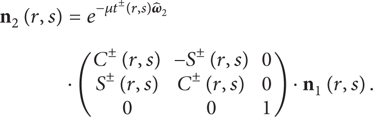
Therefore, say we have that (cos (t₀),sin(t₀)) = (C⁻(r₀,s₀),S⁻(r₀,s₀)). Then, an at least continuous function t(r,s) with ϕ(r,s,t(r,s)) = 0 for all (r,s) ∈ U and with t(r₀,s₀) = t₀ satisfies

(\cos (t (r, s)), \sin (t (r, s))) = (C^{-} (r, s), S^{-} (r, s)) \forall (r, s) \in U,

(30)

as the change of the sign of the square root is only possible at points (r,s) with Δ(r,s) = 0. Locally at (r₀,s₀), the function t(r,s) can be obtained by applying an “intelligent” arctan to (30). Globally, the existence of t(r,s) cannot be guaranteed in general: the map t:U → R is a lifting of the map U → S₁;(r,s)↦(C⁻(r,s),S⁻(r,s)) with respect to the usual covering map R → S₁ of the circle S₁. However, such lifting always exists for convex domains U.

If t(r,s) exists on U, then we obtain a C¹-parameterization:

G_{2} (r, s) = e^{- μ t (r, s) {\hat{ξ}}_{2}} e^{t {(r, s) \hat{ξ}}_{1}} G_{1} (r, s),

(31)

which describes the surface Γ₂. Note that the equation of meshing is automatically fulfilled, but G₂(r,s) may not be a regular parameterization.

4. Bevel Gear Drives

We consider a bevel gear drive consisting of a gear Γ₁ and the (theoretical) pinion Γ₂. We retain all notations of Section 3. Moreover, we choose the intersection point of the axes of the gear and the pinion as the origin of the spatial frame. Then we have that v ₁ = v ₂ = 0. By choosing the axes of the spatial frame, we achieve that ω₁ = (0, 0, 1) and that ω₂ = (sin σ,0, cos σ), where σ denotes the shaft angle; see Figure 3.

Figure 3:

Settings of the bevel gear drive.

Moreover, let

\begin{array}{l} h_{1} (r, s) = (a (r, s), b (r, s), c (r, s)) \\ = g_{1} (r, s) \land n_{1} (r, s) \\ = 〈 g_{1} ∣ \frac{\partial g_{1}}{\partial s} 〉 \cdot \frac{\partial g_{1}}{\partial r} - 〈 g_{1} ∣ \frac{\partial g_{1}}{\partial r} 〉 \cdot \frac{\partial g_{1}}{\partial s} \\ = \frac{1}{2} \cdot (\frac{\partial {| g_{1} |}^{2}}{\partial s} \frac{\partial g_{1}}{\partial r} - \frac{\partial {| g_{1} |}^{2}}{\partial r} \frac{\partial g_{1}}{\partial s}), \\ ν ≔ \frac{μ \cos σ - 1}{μ \sin σ} . \end{array}

(32)

We compute ${\overset{⁁}{ω}}_{1} ω_{2} = (0, \sin σ, 0)$ , ${\overset{⁁}{ω}}_{1}^{2} ω_{2} = (- \sin σ, 0, 0)$ , and 〈ω₁ ∣ ω₂〉 = cos σ. Dividing (21) by $\sin σ$ leads to

- a (r, s) \cos (t) + b (r, s) \sin (t) = ν c (r, s) .

(33)

Thus, if $Δ (r, s) = a {(r, s)}^{2} + b {(r, s)}^{2} - ν^{2} c {(r, s)}^{2}$ is strictly positive, then (33) is solved by

\begin{matrix} \cos (t) = C^{\pm} (r, s) = \frac{- ν a c \pm b \sqrt{Δ}}{a^{2} + b^{2}}, \\ \sin (t) = S^{\pm} (r, s) = \frac{ν b c \pm a \sqrt{Δ}}{a^{2} + b^{2}} . \end{matrix}

(34)

If we are dealing with one tooth flank only, then we may achieve that t is between − π/2 and π/2 by taking an appropriate time offset. A short computation leads to the following explicit formula:

t = t^{\pm} (r, s) = \arctan (\frac{a (r, s) b (r, s) \pm c (r, s) \sqrt{Δ (r, s)}}{a {(r, s)}^{2} - ν^{2} c {(r, s)}^{2}}) .

(35)

Consequently, the mating pinion Γ₂ is given by

g_{2} (r, s) = e^{- μ t^{\pm} (r, s) {\hat{ω}}_{2}} \cdot (\begin{pmatrix} C^{\pm} (r, s) & - S^{\pm} (r, s) & 0 \\ S^{\pm} (r, s) & C^{\pm} (r, s) & 0 \\ 0 & 0 & 1 \end{pmatrix}) \cdot g_{1} (r, s);

(36)

note that this may not be a regular parameterization. If Γ₂ has a normal at its point G₂(r,s), then the normal is given by

n_{2} (r, s) = e^{- μ t^{\pm} (r, s) {\hat{ω}}_{2}} \cdot (\begin{pmatrix} C^{\pm} (r, s) & - S^{\pm} (r, s) & 0 \\ S^{\pm} (r, s) & C^{\pm} (r, s) & 0 \\ 0 & 0 & 1 \end{pmatrix}) \cdot n_{1} (r, s) .

(37)

The results obtained so far can be applied to the remanufacturing of the pinion of a bevel gear drive. To this end, one measures the tooth of the existing gear by a 3D-coordinate measuring machine and obtains a set of points $g_{1}^{(j)}$ , j = 1,…,n, of the tooth in Euclidean coordinates. The corresponding normals $n_{1}^{(j)}$ , j = 1,…,n, can either be measured, too, or can be derived from the point cloud by applying tools from image geometry; a typical result (with reduced number of points) of such a measurement is given in Figure 4. A crucial condition for the quality of the replacement pinion is the measurement of sufficiently many points. Experiments show that about 100 points/mm² lead to satisfactory results.

Figure 4:

Measured point cloud and normals of a gear tooth flank.

After having performed the measurement, we compute $h_{1}^{(j)} = g_{1}^{(j)} \land n_{1}^{(j)}$ and then the instant $t = t^{(j)}$ at which the point $g_{1}^{(j)}$ is in contact with the pinion; see (35). Applying formulas (36) and (37) yields the results

g_{2}^{(j)}, n_{2}^{(j)}, t^{(j)}, j = 1, \dots, n,

(38)

where $g_{2}^{(j)}$ is the point of the mating pinion which is in contact with $g_{1}^{(j)}$ at $t = t^{(j)}$ and $n_{2}^{(j)}$ is the corresponding normal of the pinion's tooth flank. If we consider the real-valued function

λ : {\tilde{Γ}}_{2} = {g_{2}^{(j)} ∣ j = 1, \dots, n} ⟶ R; λ (g_{2}^{(j)}) = t^{(j)}

(39)

on the discrete point set ${\tilde{Γ}}_{2}$ , then the instantaneous contact lines (i.e., the curves at which the pinion is in contact with the gear at a certain instant t = t₀) are the level sets of λ. This fact makes the computation of the instantaneous contact lines accessible for fast algorithms from discrete geometry. Figure 5 shows the result of such a computation.

Figure 5:

Instantaneous contact lines on the computed pinion.

We obtained the theoretical pinion belonging to the existing gear so far. By an appropriate tooth surface modification, we can improve the meshing performance of the gear drive, cp. [5] for the techniques used in this step. Finally, the pinion is produced on a CNC machining center; therefore, one can benefit from the description of the surface in terms of Euclidean coordinates.

5. Generation of Spiral Bevel Gears by Special Machine Tools

The objective of this section is to derive a parameterization of the gear tooth surface produced by a face hobbing machine. The blade of the head cutter performs a rotation, which is given by an infinitesimal rotation ξ_b = (ω_b, v _b) ∈ se(3) with |ω_b| = 1 and 〈ω_b ∣ v _b〉 = 0 in the initial position. We will describe the blade by a curve

B (s) = (\begin{pmatrix} ω_{b} \land v_{b} + b (s) \\ 1 \end{pmatrix})

(40)

and require that B(s) does not intersect the axis ω_b∧ v _b + R·ω_b; that is, b (s) and ω_b are linearly independent. Performing the rotation of the head cutter, we obtain a surface of revolution

Γ_{1} : G_{1} (s, θ) = (\begin{pmatrix} g_{1} (s, θ) \\ 1 \end{pmatrix}) = (\begin{pmatrix} ω_{b} \land v_{b} + e^{θ {\hat{ω}}_{b}} b (s) \\ 1 \end{pmatrix}),

(41)

which we will refer to as the generating surface. Since the head cutter is installed on the rotating cradle, it performs a rotation itself, which is given by ξ₁ = (ω₁, v ₁) ∈ se(3) with |ω₁| = 1 and 〈ω₁ ∣ v ₁〉 = 0. Moreover, we let the rotation of the gear blank be given by ξ₂ = (ω₂, v ₂) ∈ se(3) (again |ω₂| = 1 and 〈ω₂ ∣ v ₂〉 = 0); the ratio of angular velocities of the rotations of the cradle and the gear blank will be denoted by μ. 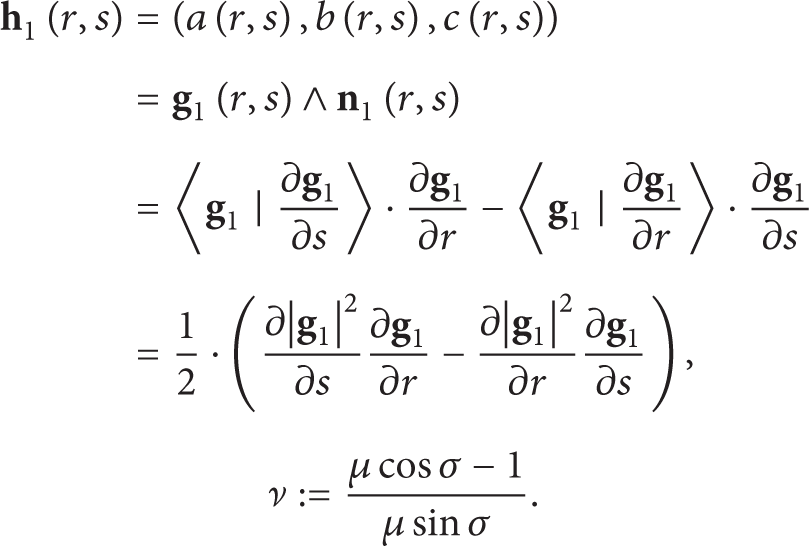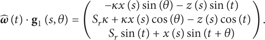We agree on the usual assumption that the blade rotation does not influence the gear generation; that is, the gear tooth surface Γ₂ will be the envelope of the family $F (s, θ, t) = e^{- μ t {\overset{⁁}{ξ}}_{2}} e^{t {\overset{⁁}{ξ}}_{1}} G_{1} (s, θ)$ .

The vector n _b(s) = b ′(s)∧(ω_b∧ b (s)) = 〈 b (s) ∣ b ′(s)〉ω_b − 〈ω_b ∣ b ′(s)〉 b (s) is perpendicular to the surface Γ₁ at the point G₁(s,0) = B(s). Since b (s) and ω_b are linearly independent, n _b(s) does not vanish. Consequently, the vector

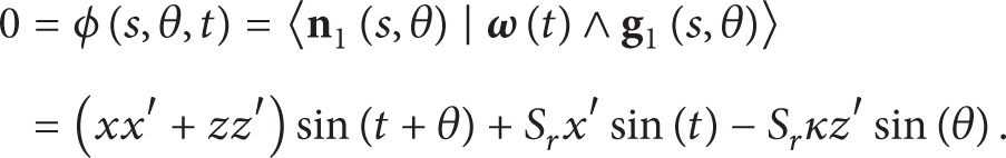
n_{1} (s, θ) = e^{θ {\hat{ω}}_{b}} \cdot n_{b} (s) = 〈 b (s) ∣ b^{'} (s) 〉 ω_{b} - 〈 ω_{b} ∣ b^{'} (s) 〉 e^{θ {\hat{ω}}_{b}} b (s) \neq 0

(42)

is parallel to the normal of Γ₁ at G₁(s,θ). Putting $ξ (t) = (ω (t), v (t)) = ξ_{1} - {Ad}_{e^{- t {\overset{⁁}{ξ}}_{1}}} ξ_{2}$ leads to the equation of meshing:

ϕ (s, θ, t) = 〈 n_{1} (s, θ) ∣ ω (t) \land g_{1} (s, θ) + v (t) 〉 = 0,

(43)

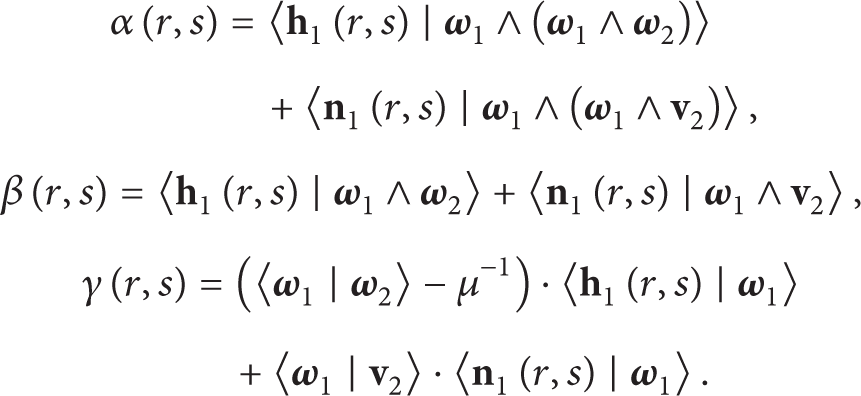
cp. (17). A straight-forward computation shows that

0 = ϕ (s, θ, t) = α (s, t) \cos (θ) + β (s, t) \sin (θ) - γ (s, t),

(44)

where

\begin{matrix} α (s, t) = - 〈 b ∣ b^{'} 〉 〈 {\hat{ω}}_{b} b ∣ ω 〉 - 〈 {\hat{ω}}_{b} b ∣ {\hat{v}}_{b} b^{'} 〉 〈 ω_{b} ∣ ω 〉 + 〈 ω_{b} ∣ b^{'} 〉 〈 {\hat{ω}}_{b}^{2} b ∣ v 〉, \\ β (s, t) = - 〈 b ∣ b^{'} 〉 〈 {\hat{ω}}_{b}^{2} b ∣ ω 〉 + 〈 {\hat{ω}}_{b} b ∣ (ω_{b} \land v_{b}) \land b^{'} 〉 〈 ω_{b} ∣ ω 〉 - 〈 ω_{b} ∣ b^{'} 〉 〈 {\hat{ω}}_{b} b ∣ v 〉, \\ γ (s, t) = (〈 v_{b} ∣ ω 〉 + 〈 ω_{b} ∣ v 〉) 〈 {\hat{ω}}_{b}^{2} b ∣ b^{'} 〉 . \end{matrix}

(45)

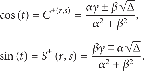
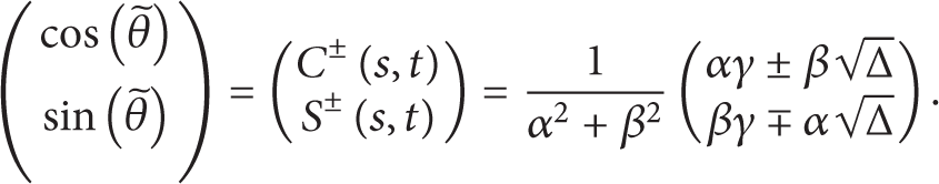
We reuse the arguments given in Section 3 and obtain the following: as long as Δ≔α² + β² − γ² is strictly positive, (44) has precisely two solutions (cos (θ), sin(θ)), namely,

\begin{matrix} \cos (θ) = C^{\pm} (s, t) = \frac{α γ \pm β \sqrt{Δ}}{α^{2} + β^{2}}, \\ \sin (θ) = S^{\pm} (s, t) = \frac{β γ \mp α \sqrt{Δ}}{α^{2} + β^{2}} . \end{matrix}

(46)

By Rodrigues’ formula, we can write the corresponding rotation $e^{θ {\overset{⁁}{ω}}_{b}}$ as a function of (s,t):

R^{\pm} (s, t) = I_{3} + S^{\pm} (s, t) {\hat{ω}}_{b} + (1 - C^{\pm} (s, t)) {\hat{ω}}_{b}^{2} .

(47)

Therefore, the envelope Γ₂ in question is contained in the surface with the parameterization

G_{2} (s, t) = e^{- μ t {\hat{ξ}}_{2}} e^{t {\hat{ξ}}_{1}} (\begin{pmatrix} ω_{b} \land v_{b} + R^{\pm} (s, t) b (s) \\ 1 \end{pmatrix}),

(48)

whence we obtained an explicit description of this surface in Euclidean coordinates. It is worth noting that the normal of Γ₂ at the point G₂(r,s) is given by

n_{2} (s, t) = (\begin{pmatrix} e^{- μ t {\hat{ω}}_{2}} e^{t {\hat{ω}}_{1}} R^{\pm} (s, t) b (s) \\ 0 \end{pmatrix}),

(49)

provided that the parameterization given by (48) is regular at (s,t).

5.1. Plane Blades

We retain the preceding notations and conventions. Additionally, we require that the blade curve ω_b∧ v _b + b (s) and the axis ω_b∧ v _b + R·ω_b are contained in the same plane. We choose a right-handed coordinate system (μ_b,η_b,ω_b) such that ν_b = r·μ_b holds for some r ≥ 0. By taking an appropriate offset for θ we may achieve that

b (s) = x (s) μ_{b} + z (s) ω_{b}, where x (s) > 0 \forall s;

(50)

recall that the blade curve does not intersect the axis of the head cutter. Dividing (44) by x(s) yields

0 = \tilde{ϕ} (s, θ, t) = \tilde{α} (s, t) \cos (θ) + \tilde{β} (s, t) \sin (θ) - \tilde{γ} (s, t),

(51)

where

\begin{matrix} \tilde{α} (s, t) = - (x x^{'} + z z^{'}) \cdot 〈 η_{b} ∣ ω 〉 + r z^{'} \cdot 〈 ω_{b} ∣ ω 〉 - z^{'} \cdot 〈 μ_{b} ∣ v 〉, \\ \tilde{β} (s, t) = (x x^{'} + z z^{'}) \cdot 〈 μ_{b} ∣ ω 〉 - z^{'} \cdot 〈 η_{b} ∣ v 〉, \\ \tilde{γ} (s, t) = - r x^{'} \cdot 〈 μ_{b} ∣ ω 〉 - x^{'} \cdot 〈 ω_{b} ∣ v 〉 . \end{matrix}

(52)

For computational purposes, it is useful to know that

(\begin{pmatrix} \tilde{α} \\ \tilde{β} \end{pmatrix}) = (\begin{pmatrix} r 〈 ω_{b} ∣ ω 〉 z^{'} \\ 0 \end{pmatrix}) - (\begin{pmatrix} 〈 η_{b} ∣ ω 〉 & 〈 μ_{b} ∣ v 〉 \\ - 〈 μ_{b} ∣ ω 〉 & 〈 η_{b} ∣ v 〉 \end{pmatrix}) \cdot (\begin{pmatrix} x x^{'} + z z^{'} \\ z^{'} \end{pmatrix}) .

(53)

5.2. Generation of the Gear

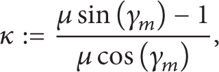
For the generation of the gear of a spiral bevel gear drive, the axes of the cradle and of the head cutter are chosen to be parallel, whence we may take ω₁ = ω_b = (0, 0, 1). As usual, the blank offset and the machine center to back are set to 0. Therefore, the axes of the cradle and of the gear blank meet. We choose the intersection point to be the origin of the coordinate frame and, hence, obtain that v ₁ = v ₂ = 0. Moreover, the so-called cradle angle q₂ simply is an offset for the cradle rotation, so we can neglect it, too. Finally, we arrange the x-axis of the coordinate system in a way such that ω₂ = (cos (γ_m), 0, sin (γ_m)), where γ_m is the root angle of the machine tool. Figure 6 contains the basic settings defined so far.

Figure 6:

Settings of the machine tool.

The plane blade of the head cutter is given by the curve

\begin{matrix} B (s) = (\begin{pmatrix} b (s) \\ 1 \end{pmatrix}), where b (s) = (S_{r} + x (s), 0, z (s)) \\ with x (s) > 0 . \end{matrix}

(54)

Here, S_r denotes the radial setting. Rotating B(s) around the axis of the head cutter yields the following parameterization of the generating surface Γ₁:

g_{1} (s, θ) = (S_{r} + x (s) \cos (θ), x (s) \sin (θ), z (s)) .

(55)

The following vector is parallel to the normal of Γ₁ at g₁(s,θ):

\begin{array}{l} n_{1} (s, θ) = \frac{1}{x (s)} \cdot (\frac{\partial g_{1}}{\partial s} \land \frac{\partial g_{1}}{\partial θ}) \\ = (- z^{'} (s) \cos (θ), - z^{'} (s) \sin (θ), x^{'} (s)) . \end{array}

(56)

A short computation shows that the family (14) of surfaces is given by

f (s, θ, t) = T^{- 1} (\begin{pmatrix} \cos (μ t) & \sin (μ t) & 0 \\ - \sin (μ t) & \cos (μ t) & 0 \\ 0 & 0 & 1 \end{pmatrix}) \times T (\begin{pmatrix} S_{r} \cos (t) + \cos (t + θ) \cdot x (s) \\ S_{r} \sin (t) + \sin (t + θ) \cdot x (s) \\ z (s) \end{pmatrix}),

(57)

where

T = (\begin{pmatrix} \sin (γ_{m}) & 0 & - \cos (γ_{m}) \\ 0 & 1 & 0 \\ \cos (γ_{m}) & 0 & \sin (γ_{m}) \end{pmatrix}) .

(58)

Putting

κ ≔ \frac{μ \sin (γ_{m}) - 1}{μ \cos (γ_{m})},

(59)

we easily derive $ω_{1} - μ ω_{2} = - μ \cos (γ_{m}) \cdot {(1, 0, κ)}^{T}$ . Up to a constant scalar, we can take $ω (t) = e^{- t {\overset{⁁}{ω}}_{1}} \cdot {(1, 0, κ)}^{T} = {(\cos (t), - \sin (t), κ)}^{T}$ , which in turn leads to

\hat{ω} (t) \cdot g_{1} (s, θ) = (\begin{pmatrix} - κ x (s) \sin (θ) - z (s) \sin (t) \\ S_{r} κ + κ x (s) \cos (θ) - z (s) \cos (t) \\ S_{r} \sin (t) + x (s) \sin (t + θ) \end{pmatrix}) .

(60)

We obtain the equation of meshing (up to a constant factor) as follows:

\begin{matrix} 0 = ϕ (s, θ, t) = 〈 n_{1} (s, θ) ∣ ω (t) \land g_{1} (s, θ) 〉 \\ = (x x^{'} + z z^{'}) \sin (t + θ) + S_{r} x^{'} \sin (t) - S_{r} κ z^{'} \sin (θ) . \end{matrix}

(61)

Putting $\tilde{θ} ≔ θ + t$ , we can rewrite the latter equation as

α (s, t) \cos (\tilde{θ}) + β (s, t) \sin (\tilde{θ}) - γ (s, t) = 0,

(62)

where

\begin{matrix} α (s, t) = S_{r} κ z^{'} \sin (t), \\ β (s, t) = x x^{'} + z z^{'} - S_{r} κ z^{'} \cos (t), \\ γ (s, t) = - S_{r} x^{'} \sin (t) . \end{matrix}

(63)

This equation can be solved as before: as long as Δ = α² + β² − γ² > 0, (62) has precisely two solutions:

(\begin{pmatrix} \cos (\tilde{θ}) \\ \sin (\tilde{θ}) \end{pmatrix}) = (\begin{pmatrix} C^{\pm} (s, t) \\ S^{\pm} (s, t) \end{pmatrix}) = \frac{1}{α^{2} + β^{2}} (\begin{pmatrix} α γ \pm β \sqrt{Δ} \\ β γ \mp α \sqrt{Δ} \end{pmatrix}) .

(64)

We change the coordinate frame by retaining the origin and the y-axis and by letting ω₂ be the directional vector of the new z-axis. With respect to the new coordinate system, the parameterization of the generated gear becomes

{\bar{g}}_{2} (s, t) = (\begin{pmatrix} \cos (μ t) & \sin (μ t) & 0 \\ - \sin (μ t) & \cos (μ t) & 0 \\ 0 & 0 & 1 \end{pmatrix}) \cdot (\begin{pmatrix} \sin (γ_{m}) & 0 & - \cos (γ_{m}) \\ 0 & 1 & 0 \\ \cos (γ_{m}) & 0 & \sin (γ_{m}) \end{pmatrix}) \cdot (\begin{pmatrix} S_{r} \cos (t) + C^{\pm} (s, t) x (s) \\ S_{r} \sin (t) + S^{\pm} (s, t) x (s) \\ z (s) \end{pmatrix}) .

(65)

We point out again that ${\bar{g}}_{2} (s, t)$ exists for all (s,t) with Δ(s,t) > 0 (or with Δ(s,t) = 0 and γ(s,t)≠0), but (65) may fail to be a regular parameterization at (r,s).

5.3. Experiment

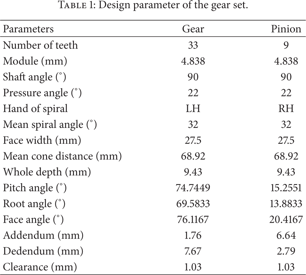
As an application, we consider a spiral bevel gear whose data stem from [1] (cp. Table 1).

Table 1:

Design parameter of the gear set.

Parameters	Gear	Pinion

Number of teeth	33	9
Module (mm)	4.838	4.838
Shaft angle (°)	90	90
Pressure angle (°)	22	22
Hand of spiral	LH	RH
Mean spiral angle (°)	32	32
Face width (mm)	27.5	27.5
Mean cone distance (mm)	68.92	68.92
Whole depth (mm)	9.43	9.43
Pitch angle (°)	74.7449	15.2551
Root angle (°)	69.5833	13.8833
Face angle (°)	76.1167	20.4167
Addendum (mm)	1.76	6.64
Dedendum (mm)	7.67	2.79
Clearance (mm)	1.03	1.03

We consider a generating tool Γ₁ with a straight blade profile and a circular fillet at the top. The geometrical parameters of the tool and the machine settings are taken from [1] again, see Table 2.

Table 2:

Tool parameters and machine settings.

Parameter	Symbol	Convex and concave side

Cutter radius (mm)	R _g	63.5
Blade angle (°)	α_g	22
Point width (mm)	P _w	2.54
Root fillet radius (mm)	ρ_w	1.524
Radial distance (mm)	S _r	64.3718
Cradle angle (°)	q	−56.78
Sliding base (mm)	ΔX_B	−0.2071
Machine root angle (°)	γ_m	69.5833
Velocity ratio	μ	1.032331

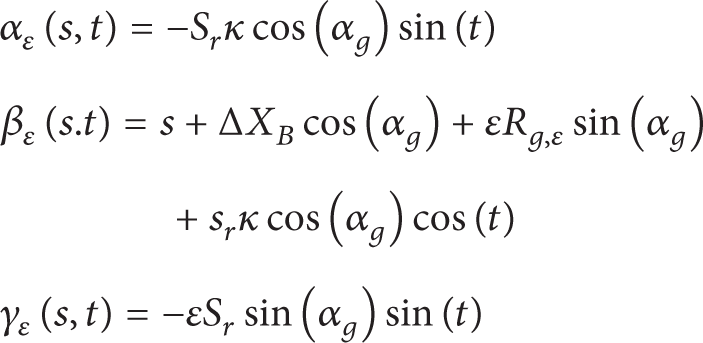
Note that both the blank offset and the machine center to back are set to 0 mm. Putting ε = + 1 for the concave side and ε = − 1 for the convex side of the tooth, the parameterization of the parts of the blade required in (54) is given by

(\begin{pmatrix} x_{ε} (s) \\ z_{ε} (s) \end{pmatrix}) = (\begin{pmatrix} R_{g, ε} + ε s \sin α_{g} \\ - Δ X_{B} - s \cdot \cos α_{g} \end{pmatrix}) with R_{g, ε} = R_{u} + ε \frac{P_{w}}{2},

(66)

(where R_g^ε is the usual cutter point radius) for the straight parts of the blade, and by

(\begin{pmatrix} x_{ε} (s) \\ z_{ε} (s) \end{pmatrix}) = (\begin{pmatrix} X_{w, ε} + ε ρ_{w} \sin s \\ - Δ X_{B} - ρ_{w} \cdot (1 - \cos s) \end{pmatrix}) with X_{w, ε} = R_{g, ε} - ε ρ_{w} \frac{1 - \sin α_{g}}{\cos α_{g}}

(67)

for the circular fillets. The coefficients in the (62) of meshing hence become

\begin{array}{l} α_{ε} (s, t) = - S_{r} κ \cos (α_{g}) \sin (t) \\ β_{ε} (s . t) = s + Δ X_{B} \cos (α_{g}) + ε R_{g, ε} \sin (α_{g}) + s_{r} κ \cos (α_{g}) \cos (t) \\ γ_{ε} (s, t) = - {ε S}_{r} \sin (α_{g}) \sin (t) \end{array}

(68)

for the straight parts and, up to the common factor ρ_w,

\begin{array}{l} α_{ε} (s, t) = - S_{r} κ \sin (s) \sin (t) \\ β_{ε} (s . t) = (Δ X_{B} + ρ_{w} + S_{r} κ \cos (t)) \cdot \sin (s) + ε X_{w, ε} \cos (s) \\ γ_{ε} (s, t) = - {ε S}_{r} \cos (s) \sin (t) \end{array}

(69)

for the circular fillets. The constant κ contained in the equations above is given by (59).

The analytic parameterization (65) of the surface has been computed by the symbolic toolbox MuPAD of MATLAB on an Intel Core i7 with 2.93 GHz and 8 GByte RAM. MuPAD prompted 0 seconds for the complete computation of the parameterization of all parts of the tooth surface. The plotting time for all five surfaces with the usual mesh of [25, 25] each took 6 seconds. The production of Figure 7 has been much more expensive (around 800 seconds for 50,000 nodes): as MuPAD cannot handle parameter sets of surfaces other than rectangular ones, one has to use quite tricky methods to restrict the surface to the body of the gear blank. However, we point out that Figure 7 is not derived from any discrete data but is a picture of the analytic surface of the gear tooth.

Figure 7:

Generated gear surface.

Finally, we remark that we are using the analytical parameterization of gears in order to obtain a point cloud describing the gear surface of appropriate precision. By overlaying random errors to the data, one can investigate the influence of errors given by measurement, by surface errors, or in algorithm used for the processing of the point cloud to the mating pinion.

6. Conclusions

An approach based on modern mechanics was proposed for the theory of gearing. Avoiding chains of coordinate systems, we achieved a more compact formulation of the theory. Moreover, the terms appearing in the equations have a precise mechanical meaning, which is independent of the coordinate frame. As a first application of the new approach, explicit formulas for the surface of a spiral bevel gear generated by a gear hobbing machine as well as for the surface of the mating pinion of an arbitrary bevel gear were given. Several computer experiments done so far show the accuracy and the effectiveness of the new approach.

Conflict of Interests

The authors declare that there is no conflict of interests regarding the publication of this paper.

Footnotes

Acknowledgments

This research has received financial support from the National Natural Science Foundation of China (no. 51205025) and was supported by the Funding Project for Academic Human Resources Development in Beijing Union University of China (BPHR2012E02), for which the authors are very appreciative.

References

Litvin

F. L.

and Fuentes

, Gear Geometry and Applied Theory, Cambridge University Press, Cambridge, UK, 2nd edition2004.

Dooner

D. B.

, The Kinematic Geometry of Gearing, John Wiley & Sons, Chichester, UK, 2nd edition2012.

di Puccio

Gabiccini

, and Guiggiani

, “Alternative formulation of the theory of gearing,” Mechanism and Machine Theory, vol. 40, no. 5, pp. 613–637, 2005.

Bullo

and Lewis

A. D.

, Geometric Control of Mechanical Systems, Springer, New York, NY, USA, 2005.

Lei

Cheng

Löwe

, and Wang

, “Remanufacturing the pinion: an application of a new design method for spiral bevel gears,” Advances in Mechanical Engineering, vol. 2014, Article ID 257581, 9 pages, 2014.

Zalgaller

V. A.

, Theory of Envelopes, Nauka, Moscow, Russia, 1991, (Russian).

Applications of the Exponential Function of the Euclidean Motion Group to the Theory of Gearing

Abstract

1. Introduction

2. Motions of the 3-Space

3. The Envelope of a Certain Family of Surfaces

3.1. Solving the Equation of Meshing

3.2. Solving for t and the Equation of the Envelope Γ2

4. Bevel Gear Drives

5. Generation of Spiral Bevel Gears by Special Machine Tools

5.1. Plane Blades

5.2. Generation of the Gear

5.3. Experiment

6. Conclusions

Conflict of Interests

Footnotes

Acknowledgments

References

3.2. Solving for t and the Equation of the Envelope Γ₂