A Formal Specification Framework for Designing and Verifying Reliable and Dependable Software for CNC Systems

Abstract

As a distributed computing system, a CNC system needs to be operated reliably, dependably, and safely. How to design reliable and dependable software and perform effective verification for CNC systems becomes an important research problem. In this paper, we propose a new modeling method called TTM/ATRTTL (timed transition models/all-time real-time temporal logics) for specifying CNC systems. TTM/ATRTTL provides full supports for specifying hard real time and feedback that are needed for modeling CNC systems. We also propose a verification framework with verification rules and theorems and implement it with STeP and SF2STeP. The proposed verification framework can check reliability, dependability, and safety of systems specified by our TTM/ATRTTL method. We apply our modeling and verification techniques on an open architecture CNC (OAC) system and conduct comprehensive studies on modeling and verifying a system controller that is the key part of OAC. The results show that our method can effectively model and verify CNC systems and generate CNC software that can satisfy system requirements in reliability, dependability, and safety.

1. Introduction

Reliability, dependability, and safety are the three most important factors in software design for computerized numerical control (CNC) systems. As a distributed computing system, a CNC system consists of a computer controller, a set of microcontrollers, and cutting tools, in which the controller can execute machine tool program and generate instructions for microcontrollers to drive the cutting tools to fabricate workpieces by selectively removing materials. Software design is extremely important to make CNC systems operate reliably, dependably, and safely, which directly influences manufacturing quality of workpieces and even the safety of operators. Therefore, how to design reliable and dependable software and perform effective verification for CNC systems becomes an important research problem.

To design such safety-critical systems, testing is not sufficient to guarantee the reliability, dependability, safety, and correctness of CNC software systems. Integrating formal specification and verification methods into software design cycle is an essential solution for quality control in CNC systems [1–3]. Hard real time and feedback, two special properties of applications in CNC systems, need to be considered when formal methods are designed. In terms of hard real time, as CNC systems are used to control machine cutting tools, almost every operation of a CNC system must be finished within a given time constraint. In terms of feedback, in order to guide cutting tools to perform directed interpolation, a lot of results generated previously are needed for generating current result. In this paper, we focus on developing a formal specification and verification frameworks by integrating hard real time and feedback with reliability, dependability, and safety for designing and verifying reliable and dependable software for CNC systems.

A lot of methods have been proposed in modeling formalisms such as finite state machines [4], statecharts [5], message sequence charts [6], and Petri nets [7]. However, the above methods cannot model real-time property efficiently. To model systems with temporal behaviors, temporal logics are the best choice which can specify system behaviors with logical formulas including temporal constraints, events, and relationships between the two [8–10]. Many different forms of temporal logics have been proposed such as PTL (propositional temporal logic) [11–15], BTTL (branching time temporal logic) [16], ITL (interval temporal logic) [17], CTL (computational tree logic) [18], RTL (real-time logic) [19, 20], LRTL (linear real-time Logic) [1–3], and RTTL (real-time temporal logic) [21]. Among them, LRTL and RTTL are most suitable to specify and verify hard real-time systems.

RTL, which is based on a first-order logic, was introduced in [19] to capture the timing requirements of real-time systems. It provides a uniform way for the specification of relative and uniform timing of events. However, the satisfiability problem for RTL, as well as for other first-order logics, is undecidable. LRTL is the extension form of RTL and can express any linear timing constraint with an arbitrary number of events variables. The way that LRTL uses to overcome the limitation of expressing the relationship between three or more events is discarding the graph form instead by a new matrices form [1], while RTTL, which is also derived from RTL, still uses the graph form, which is called the reachability graph, to express the dependencies in multievents condition [21]. However, RTTL is not good at specifying systems with feedback because there is no specification to express the past [22]. Therefore, we need new modeling formalisms to model and verify CNC systems.

In this paper, we propose a new modeling method called TTM/ATRTTL (extended timed transition models/all-time real-time temporal logics) for specifying CNC systems based on TTM/RTTL in [21, 23–30]. TTM/ATRTTL provides full support for specifying hard real time and feedback that are needed for modeling CNC systems. We also propose a verification framework with verification rules and theorems and implement it with STeP [14, 15] and SF2STeP [31, 32]. The proposed verification framework can check reliability, dependability, and safety of systems specified by our TTM/ATRTTL method. We apply our modeling and verification techniques on an open architecture CNC (OAC) system [33] and conduct comprehensive studies on modeling and verifying a system controller that is the key part of OAC. The results show that our method can effectively model and verify CNC systems and generate CNC software that can satisfy system requirements in reliability, dependability, and safety.

The rest of the paper is organized as follows. In Section 2, we propose our specification method. The formal verification framework is proposed in Section 3. In Section 4, we apply our specification and verification techniques on an open architecture CNC system. The conclusion and the future work are given in Section 5.

2. TTM/ATRTTL: A Formal Specification Method

In this section, we propose our formal specification method, TTM/ATRTTL, that can handle both hard real time and feedback. We first give background knowledge for TTMs that is used to describe reactive/real-time systems [12]. Then we propose a new declarative specification language called ATRTTL that is used to describe requirements that a TTM should satisfy.

2.1. Timed Transition Models (TTMs)

TTM is a state transition system that can be used to represent a variety of reactive, concurrent, distributed, and real-time systems. It is an extension of the fair transition systems [12] by adding time metric. The time metric with lower and upper time bounds is introduced into transitions. So it can model hard real-time behaviors of systems. Many kinds of modeling methods can be directly translated into TTMs such as real-time programs, nondeterministic timed Petri nets, and other constructs with timing properties.

Definition 1. A TTM M is defined as a seven-tuple M = (V,R,S,I,T,J,C), in which V is the variable set used to describe processes of M, R is the union of all variable types of V, S is the set of states of M and every state s in S is a mapping between variable v ∈ V and a corresponding value s(v), and I is a Boolean expression of system variables to represent the initial condition of M, T is the set of transitions, J is the weakly fair transitions set, and C is the strongly fair transitions set.

In variable set V, there are four different kinds of variables: activity variables, data variables, clock variables, and next-transition variables. Activity variable is used to represent current status of processes. Data variable can be integers, rationales, sets, or other forms of data. Clock variable is a nonnegative integer used to represent global time. Next-transition variable refers to events or transitions.

Definition 2. Transition set T is the set of all transitions of M and is defined as a four-tuple τ = (e_τ,f_τ,l_τ,u_τ).

Here, e_τ is the enable condition of transition τ. It is often expressed as enb(τ). It is a Boolean formula defined over transition variables of V. A transition τ can only be taken when the value of enb(τ) is true.

f_τ is the transformation function of transition τ. It is often expressed as upd(τ). It is a partial function to cause state transition when s(e_τ) = true is satisfied.

l_τ and u_τ are constants representing the lower and upper time bounds of transition τ. They represents that transition τ can only be taken during the interval starting from l_τ to u_τ.

There are three particular transitions:

1. tick transition: tick = (true,[t:t + 1], −, −);

2. initial transition: initial = (true,[], 0, 0);

3. spontaneous transition: spon = (e_τ,f_τ,0,∞).

If there is a transition τ from state s to state s′, then s is called the prestate of τ and s′ is called the poststate of τ, denoted as s′ ∈ τ(s).

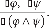
Definition 3. Transition relation is a first-order formula ρ_τ(V,V′) which relates the prestate and poststate of a transition τ. The formula is denoted as follows:

${\rho }_{\tau }\left(V,V^{\prime }\right)=\text{enb}\left(\tau \right)\wedge \text{upd}\left(\tau \right).$

(1)

Definition 4. State-assignment is the restriction of states to the domain (V − {n}) in which V is the variable set and n is next-transition variable set. The state-assignment set is denoted as S _a . State-map is the restriction of state s to the domain (V − {t,n}) in which t is time variable set. The state-map set is denoted as S _m .

Definition 5. A trajectory σ is any infinite sequence s₀s₁s₂…… of states, where s _i ∈ S (the set of all states). Let q _i be the state-assignment corresponding to a state s _i in trajectory σ; then

$\sigma =s_{\mathrm{0}}{s}_{\mathrm{1}}{s}_{\mathrm{2}}\dots =q_{\mathrm{0}}\stackrel{\hspace{0.17em}\hspace{0.17em}\hspace{0.17em}{\tau }_{\mathrm{0}}\hspace{0.17em}\hspace{0.17em}\hspace{0.17em}}{\to }{q}_{\mathrm{1}}\stackrel{\hspace{0.17em}\hspace{0.17em}\hspace{0.17em}{\tau }_{\mathrm{1}}\hspace{0.17em}\hspace{0.17em}\hspace{0.17em}}{\to }{q}_{\mathrm{2}}\stackrel{\hspace{0.17em}\hspace{0.17em}\hspace{0.17em}{\tau }_{\mathrm{2}}\hspace{0.17em}\hspace{0.17em}\hspace{0.17em}}{\to }\dots \text{.}$

(2)

Not all trajectories are actual behaviors of M. Legal trajectories are those which reflect actual behaviors of a system.

Definition 6. If there are two TTMs, M₁ and M₂, let M₁ = (V₁,R₁,S₁,I₁,T₁,J₁,C₁) and M₂ = (V₂,R₂,S₂,I₂,T₂,J₂,C₂); then

$\begin{array}{l}M=M_{\mathrm{1}}\parallel M_{\mathrm{2}}\\ \hspace{0.17em}=(V_{\mathrm{1}}\cup V_{\mathrm{2}},R_{\mathrm{1}}\cup R_{\mathrm{2}},S_{\mathrm{1}}\cup S_{\mathrm{2}},I_{\mathrm{1}}\wedge I_{\mathrm{2}},T_{\mathrm{1}}\parallel T_{\mathrm{2}},J_{\mathrm{1}}\parallel J_{\mathrm{2}},C_{\mathrm{1}}\parallel C_{\mathrm{2}})\end{array}$

(3)

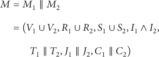
and M is still a TTM, in which one calls M₁ and M₂ as a pair of parallel TTMs.

2.2. All-Time Real-Time Temporal Logic (ATRTTL)

RTTL is used to describe requirements and operations of systems modeled by TTM. In RTTL, the temporal structure is linear and discrete. Time is defined with both a sequence of states and a sequence of temporal instants. The state-based model makes RTTL particularly suitable for model-checking techniques. A natural number is associated with each time instant, so RTTL is based on an explicit model of time. The clock in TTM/RTTL is periodically incremented and is accessible to define real-time formulas. However, there is no representation for past time in RTTL. In CNC systems, a lot of decisions are made based on the past; therefore, we propose a new temporal logic method called ATRTTL (all-time RTTL) by adding new formulas to represent past time.

To define new formulas for ATRTTL, the following operators in linear time temporal logic are used including ${}^{⫾}$ (next), ⫾ (henceforth), ⋄ (eventually), $\mathcal{U}$ (until), $\mathcal{P}$ (preceding), and $\mathcal{W}$ (waiting-for). Using these temporal operators, RTTL can give succinct, abstract formulas which support the expression of not only qualitative properties such as safety, deadlock avoidance, mutual exclusion, and liveness but also quantitative time bounds on events. Based on these operators, combining future and past temporal logics, ATRTTL (al-time real-time temporal logic), is shown in Tables 1 and 2. We call the formulas in ATRTTL as ATRTTF (all-time real-time temporal formula) that can be used to define reliability, dependability, liveness, and safety.

Table 1:

Satisfaction expressions of ATRTTL.

ATRTTF	Meaning
(σ,j) ∣ = ¬p	(σ,j) ∣ ≠p
(σ,j) ∣ = p∨q	(σ,j) ∣ = p or (σ,j) ∣ = q
(σ,j) ∣ = ⫾⫾cp	(σ,j + 1) ∣ = p and (Tj + 1 − T j )⫾c
$\left(\sigma ,j\right)\mid =p{\mathcal{U}}_{⫾\mathrm{c}}q$	For some k,j ≤ k,(σ,k) ∣ = q and (T k − T j )⫾c, and for every i,j ≤ i < k,(σ,i) ∣ = p
⋄⫾cp	${\mathrm{t}\mathrm{r}\mathrm{u}\mathrm{e}\mathcal{U}}_{⫾\mathrm{c}}p$ (eventually)
⫾⫾cp	¬⋄⫾c¬p (henceforth)
p⇒q	⫾(p → q) (entailment)
p⇔q	⫾(p↔q) (congruence)
$p{\mathcal{w}}_{⫾\mathrm{c}}q$	$⫾p\vee \left(p{\mathcal{U}}_{⫾\mathrm{c}}q\right)$ (waiting-for)
$p{\mathcal{P}}_{⫾\mathrm{c}}q$	$\neg \left(\left(\neg p\right){\mathcal{U}}_{⫾\mathrm{c}}q\right)$

Table 2:

Past operator expressions of ATRTTL.

ATRTTF	Meaning
(σ,j) ∣ = Θ⫾cp	j ≥ 1 and (σ,j − 1) ∣ = p and (T j − Tj − 1)⫾c
(σ,j) ∣ = pS⫾cq	For some k,0 ≤ k ≤ j, (σ,k) ∣ = q and (T j − T k )⫾c, and for every i,k < i ≤ j,(σ,i) ∣ = p
${\stackrel{-}{\diamond }}_{⫾c}p$	$true{\mathcal{S}}_{⫾\mathrm{c}}p$ (sometime in the past)
${\stackrel{-}{⫾}}_{⫾c}p$	$\neg {\stackrel{-}{\diamond }}_{⫾c}\neg p$ (always in the past)
$p{\mathcal{B}}_{⫾\mathrm{c}}q$	$\stackrel{-}{⫾}p\vee \left(p{\mathcal{S}}_{⫾\mathrm{c}}q\right)$ (back-to)

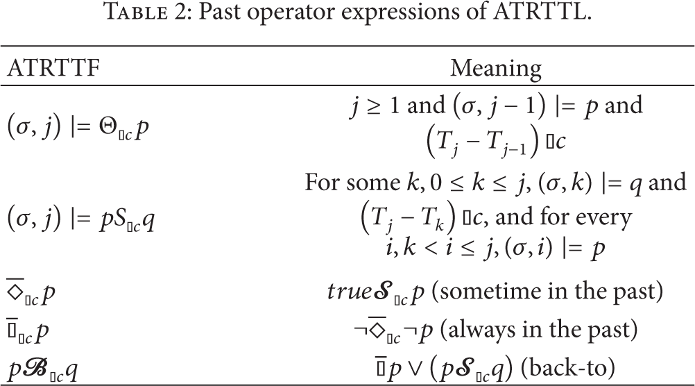
The “satisfaction” in Tables 1 and 2 is defined as follows.

Definition 7. For any trajectory σ = s₀s₁s₂…, let p and q represent the given ATRTTFs, and let (σ,j) ∣ = p represent that p holds at position j in σ; the satisfaction is given in Tables 1 and 2.

The concept of past operator expressions of ATRTTL is corresponding to the concept of normal expressions of RTTL. We introduce the past time factor, so that the whole time axis can be depicted.

3. A Formal Verification Framework with TTM/ATRTTL

In this section, we propose a formal verification framework to verify systems modeled by TTM/ATRTTL. We first propose a set of basic verification rules which can be used to simplify temporal formulas. Then we derive a set of theorems based on the verification rules which can make verification simpler.

3.1. Formal Verification Rules

First, we define verification condition as follows.

Definition 8. Verification condition is {φ}τ{ψ}, which means that whenever τ is taken from a state satisfying φ, the resulting state must satisfy ψ. If φ itself is the only resulting state, then the verification condition will be given by {φ}τ{φ}.

Based on Definition 8, we give a set of verification rules which are the basis of the theorems in Section 3.2. The most important feature of verification rules is that it can convert a given temporal logic formula to simple first-order formulas that can be easily verified.

Giving an initial condition I, a transition set T, and ATRTTFs φ and ψ, the verification rules are as follows.

Rule 1 (INV). INV for ATRTTF φ:

$\frac{\begin{array}{c}I\mathrm{1}:I⟶\phi \\ I\mathrm{2}:\left\{\phi \right\}T\left\{\phi \right\}\end{array}}{▯\phi }.$

(4)

Premise I1 means that the initial condition implies formula φ. Premise I2 means the verification condition {φ}τ{φ} holds. The conclusion is that formula φ is henceforth satisfied.

Rule 2 (MON). MON for ATRTTF φ and ψ:

$\frac{\begin{array}{cc}▯\phi ,& \phi ⟶\psi \end{array}}{▯\psi }.$

(5)

Rule MON means if we can prove the henceforth property of formula φ by INV and we can imply the ψ from φ, then the conclusion is that formula ψ is henceforth valid. By applying Rule 2, we can convert a complicated assertion to a simpler one that can be proved first.

Rule 3 (CON). CON for ATRTTF φ and ψ:

$\frac{\begin{array}{cc}▯\phi ,& ▯\psi \end{array}}{▯\left(\phi \wedge \psi \right)}.$

(6)

Rule CON means that, by proving the henceforth property of relative simple ATRTTFs, we can prove a more complicated one.

Rule 4 (INC). INC For ATRTTF φ,ψ, and χ:

$\frac{\begin{array}{cc}▯\chi ,& ▯\left(\chi \wedge \left(\phi ⟶\psi \right)\right)\end{array}}{▯\left(\phi ⟶\psi \right)}.$

(7)

The INC rule means if we can prove the henceforth validity of ATRTTF χ, and an augmented implication χ∧(φ → ψ), then we can get the henceforth property of implication φ → ψ.

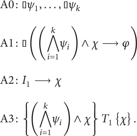
Rule 5 (GEN). GEN for ATRTTF φ,χ, and ψ₁,…,ψ _k :

$\frac{\begin{array}{c}\text{G}\mathrm{0}:▯{\psi }_{\mathrm{1}},\dots ,▯{\psi }_k\hfill \\ \text{G}\mathrm{1}:▯\left(\left(\underset{i=\mathrm{1}}{\overset{k}{\bigwedge }}{\psi }_i\right)\wedge \chi ⟶\phi \right)\hfill \\ \text{G}\mathrm{2}:I⟶\chi \hfill \\ \text{G}\mathrm{3}:\left\{\left(\underset{i=\mathrm{1}}{\overset{k}{\bigwedge }}{\psi }_i\right)\wedge \chi \right\}T\left\{\chi \right\}\hfill \end{array}}{▯\phi }.$

(8)

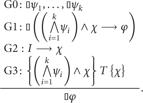
The GEN rule is a generalized form of RULE INC. It means, if we can prove a series of ATRTTF ψ₁,…,ψ _k and the augmented implication (⋀_{i = 1} ^k ψ _i )∧χ → φ, the initial condition implies formula χ, and the verification condition {(⋀_{i = 1} ^k ψ _i )∧χ}T{χ} holds; then we can get the validity of henceforth property of ATRTTF φ.

Rule 6 (WAIT). WAIT for ATRTTF φ,ψ:

$\frac{\begin{array}{c}\text{W}\mathrm{1}:I⟶\phi \vee \psi \\ \text{W}\mathrm{2}:\left\{\phi \right\}\tau \left\{\phi \vee \psi \right\}\end{array}}{\phi w\psi }.$

(9)

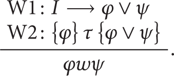
The WAIT rule means if any state satisfying the initial condition implies ATRTTFs φ and ψ and the verification condition {φ}τ{φ∨ψ} is also satisfied, then we can get the waiting-for formula φwψ.

Rule 7 (NEST-WAIT). NEST for ATRTTF φ _n ,…,φ₀:

$\frac{\begin{array}{c}\text{W}\mathrm{1}:I⟶{{\displaystyle \bigvee }}_{j=\mathrm{0}}^i{\phi }_j\hfill \\ \text{W}\mathrm{2}:\left\{{\phi }_i\right\}T\left\{{{\displaystyle \bigvee }}_{j=\mathrm{0}}^i{\phi }_j\right\}\hspace{1em}\text{for}\hspace{0.17em}\hspace{0.17em}i=\mathrm{1},\dots ,n\hfill \end{array}}{{\phi }_{n}w{\phi }_{n-\mathrm{1}}\cdots {\phi }_{\mathrm{1}}w{\phi }_{\mathrm{0}}}.$

(10)

The NEST-WAIT rule is a generalized form of RULE WAIT. It means if any state satisfying the initial condition implies a series of φ _i and every φ _i is followed by a φ _j (i ≥ j), then we can get the nested waiting-for ATRTTF φ _n wφ_{n − 1}⋯φ₁wφ₀.

Rule 8 (STRONG-NEST-WAIT). STRONG for ATRTTF φ _n ,…,φ₀:

$\frac{\begin{array}{c}\text{S}\mathrm{1}:I⟶{{\displaystyle \bigvee }}_{j=\mathrm{0}}^n{\phi }_j\hfill \\ \text{S}\mathrm{2}:\left\{{\phi }_i\right\}T\left\{{{\displaystyle \bigvee }}_{j=\mathrm{0}}^i{\phi }_j\right\}\hspace{1em}\text{for}\hspace{0.17em}\hspace{0.17em}i=\mathrm{1},\dots ,n\hfill \\ \text{S}\mathrm{3}:{\phi }_i⟶{\psi }_i\hspace{1em}\text{for}\hspace{0.17em}\hspace{0.17em}i=\mathrm{0},\dots ,n\hfill \end{array}}{{\psi }_{n}w{\psi }_{n-\mathrm{1}}\cdots {\psi }_{\mathrm{1}}w{\psi }_{\mathrm{0}}}.$

(11)

The STRONG-NEST-WAIT rule is a more generalized form of RULE NEST-WAIT. It adds the assertion S3 to NEST-WAIT in such a way that we can get a complicated assertion waiting-for ATRTTF ψ _n wψ_{n − 1}⋯ψ₁wψ₀ by a relative simple one φ _n wφ_{n − 1}⋯φ₁wφ₀.

Rule 9 (CHAIN). CHAIN for ATRTTF φ:

$\frac{\begin{array}{c}\text{C}\mathrm{1}:I⟶\phi \hfill \\ \text{C}\mathrm{2}:\left\{\phi \right\}T\left\{q\right\}\hfill \end{array}}{\diamond q}.$

(12)

The CHAIN rule means if we can prove φ from the initial condition and the verification condition {φ}T{q} is valid, then we can get the eventuality ATRTTF ⋄q.

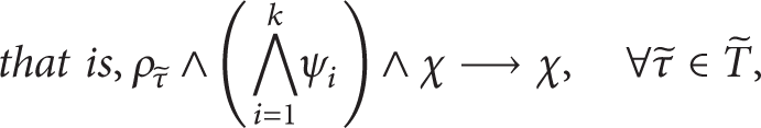
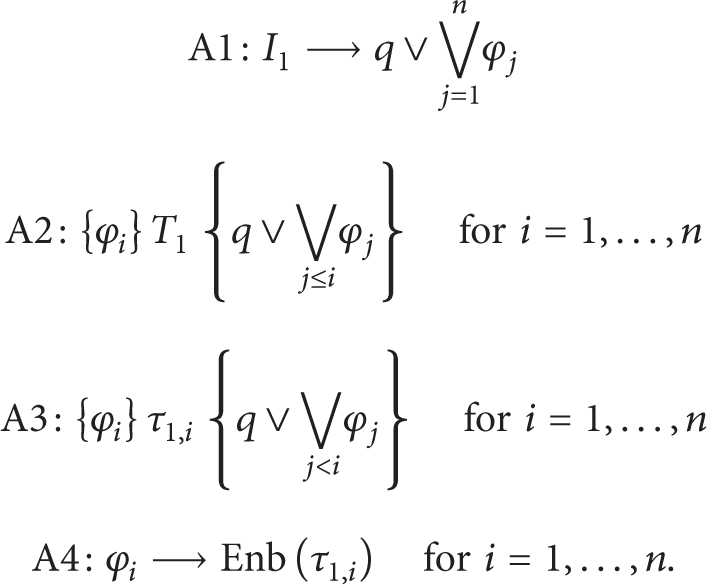
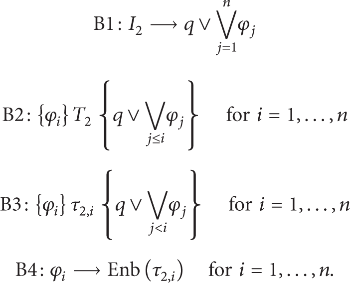
Rule 10 (NEST-CHAIN). NEST-CHAIN for ATRTTF φ _n ,…,φ₁ and transitions τ _n ,…,τ₁:

$\frac{\begin{array}{c}\text{C}\mathrm{1}:I⟶q\vee \underset{j=\mathrm{1}}{\overset{n}{{\displaystyle \bigvee }}}{\phi }_j\hfill \\ \text{C}\mathrm{2}:\left\{{\phi }_i\right\}T\left\{q\vee \underset{j\le i}{{\displaystyle \bigvee }}{\phi }_j\right\}\hspace{1em}\text{for}\hspace{0.17em}\hspace{0.17em}i=\mathrm{1},\dots ,n\hfill \\ \text{C}\mathrm{3}:\left\{{\phi }_i\right\}{\tau }_i\left\{q\vee \underset{j<i}{{\displaystyle \bigvee }}{\phi }_j\right\}\hspace{1em}\text{for}\hspace{0.17em}\hspace{0.17em}i=\mathrm{1},\dots ,n\hfill \\ \text{C}\mathrm{4}:{\phi }_i\to \text{Enb}\left({\tau }_i\right)\hspace{1em}\text{for}\hspace{0.17em}\hspace{0.17em}i=\mathrm{1},\dots ,n\hfill \end{array}}{\diamond q}.$

(13)

The NEST-CHAIN ATRTTF is a more generalized form of RULE CHAIN. Premise C1 means initial condition I implies q or one of the ATRTTFs φ _i . C2 means the verification condition {φ _i }T{q∨⋁_{j ≤ i}φ _j } is valid for every φ _i . C3 means that the verification condition satisfies the “just” property. And C4 means that, at each φ _i , the just transition τ _i is enabled. With these four premises, we can get the more generalized eventuality ATRTTF ⋄q.

3.2. Theorems Based on Verification Rules

Based on the verification rules above, we derive a set of theorems that can simplify complicated systems or specifications for easy verification based on theorems in [31]. We first define closed-loop TTM and then present four theorems.

Definition 9. A closed-loop TTM is a three-tuple CT = (O,S,C), in which O represents the TTM for the controlled object of a system, S represents the required specifications of a system in ATRTTL, and C represents the TTM of the system controller. CT means that O can work under C in the manner of what S requires.

Based on the above definition, we give two CT s. One is simple and the other is complicated. The set of theorems below are used to construct a complicated CT based on a simple CT with easy transferring procedures. The theorems are separated into three categories: invariance set, eventuality set, and sequence set. We first present a premise that is used for all theorems.

Premise. Suppose we have two closed-loop TTMs CT₁ = (O₁,S₁,C₁) and CT₂ = (O₂,S₂,C₂) where CT₁ and CT₂ have underlying TTM representations M₁ = [O₁∥C₁] = (V₁,R₁,S₁,I₁,T₁,J₁,C₁) and M₂ = [O₂∥C₂] = (V₂,R₂,S₂,I₂,T₂,J₂,C₂). Let $\tilde{T}=T_{\mathrm{2}}-T_{\mathrm{1}}$ , just transition, $\tilde{\tau }={\tau }_{\mathrm{2}}-{\tau }_{\mathrm{1}}$ , V₁⊆V₂, R₁≡R₂, S₁⊆S₂, I₂ → I₁, T₁⊆T₂, J₁⊆J₂, and C₁⊆C₂.

Theorem 10 (invariance 1). CT₂ satisfies ATRTTF M₂ ∣ = ⫾φ if CT₁ satisfies M₁ ∣ = ⫾φ and the proof obligations Δ1 and Δ2 hold, where

$\begin{array}{c}\mathrm{\Delta }\mathrm{1}:▯\left(\left(\neg I_{\mathrm{2}}\wedge I_{\mathrm{1}}\wedge \neg \chi \right)\vee \left(I_{\mathrm{2}}\wedge \neg I_{\mathrm{1}}\wedge \chi \right)\right)\\ \mathrm{\Delta }\mathrm{2}:\left\{\left(\underset{i=\mathrm{1}}{\overset{k}{\bigwedge }}{\psi }_i\right)\wedge \chi \right\}\tilde{T}\left\{\chi \right\},\\ that\hspace{0.17em}is,{\rho }_{\tilde{\tau }}\wedge \left(\underset{i=\mathrm{1}}{\overset{k}{\bigwedge }}{\psi }_i\right)\wedge \chi ⟶\chi ,\hspace{1em}\forall \tilde{\tau }\in \tilde{T},\end{array}$

(14)

in which ψ _i and χ are defined in GEN rule.

Proof. Because M₁ ∣ = ⫾φ, from GEN rule, we can get

$\begin{array}{c}\text{A}\mathrm{0}:▯{\psi }_{\mathrm{1}},\dots ,▯{\psi }_k\hfill \\ \text{A}\mathrm{1}:▯\left(\left(\underset{i=\mathrm{1}}{\overset{k}{\bigwedge }}{\psi }_i\right)\wedge \chi ⟶\phi \right)\hfill \\ \text{A}\mathrm{2}:I_{\mathrm{1}}⟶\chi \hfill \\ \text{A}\mathrm{3}:\left\{\left(\underset{i=\mathrm{1}}{\overset{k}{\bigwedge }}{\psi }_i\right)\wedge \chi \right\}{T}_{\mathrm{1}}\left\{\chi \right\}.\hfill \end{array}$

(15)

In order to prove M₂ ∣ = ⫾φ, we should establish four condition expressions as given by GEN rule. Consider the following:

$\begin{array}{c}\text{B}\mathrm{0}:▯{\psi }_{\mathrm{1}},\dots ,▯{\psi }_k\hfill \\ \text{B}\mathrm{1}:▯\left(\left(\underset{i=\mathrm{1}}{\overset{k}{\bigwedge }}{\psi }_i\right)\wedge \chi ⟶\phi \right)\hfill \\ \text{B}\mathrm{2}:I_{\mathrm{2}}⟶\chi \hfill \\ \text{B}\mathrm{3}:\left\{\left(\underset{i=\mathrm{1}}{\overset{k}{\bigwedge }}{\psi }_i\right)\wedge \chi \right\}{T}_{\mathrm{2}}\left\{\chi \right\}.\hfill \end{array}$

(16)

Obviously, A0 → B0, A1 → B1. Then we focus on B2 and B3. From Δ1 and A2, we can get

$\text{A}\mathrm{2}\wedge \mathrm{\Delta }\mathrm{1}=\left(\left(\neg I_{\mathrm{1}}\vee \chi \right)\wedge \left(\neg I_{\mathrm{2}}\wedge I_{\mathrm{1}}\wedge \neg \chi \right)\vee \left(I_{\mathrm{2}}\wedge \neg I_{\mathrm{1}}\wedge \chi \right)\right)⟷\left(I_{\mathrm{2}}⟶\chi \right)⟷\text{B}\mathrm{2}$

(17)

and Δ2∧A3↔B3. B0, B1, B2, and B3 have all been proved. Hence the invariance theorem is proved.

Using Theorem 10, when proving an invariance of a more complicated system, we only need to deal with the additional initial states and the transitions rather than the whole incremental system.

Theorem 11 (invariance 2). CT2 satisfies ATRTTF M₂ ∣ = ⫾(φ₁∧φ₂) if CT₁ satisfies M₁ ∣ = ⫾φ₁ and the proof obligations Δ1,Δ2,Δ3, and Δ4 hold, where

$\begin{array}{c}\mathrm{\Delta }\mathrm{1}:▯\left(\left(\neg I_{\mathrm{2}}\wedge I_{\mathrm{1}}\wedge \neg {\phi }_{\mathrm{1}}\right)\vee \left(I_{\mathrm{2}}\wedge \neg I_{\mathrm{1}}\wedge {\phi }_{\mathrm{1}}\right)\right)\hfill \\ \mathrm{\Delta }\mathrm{2}:\left\{{\phi }_{\mathrm{1}}\right\}\tilde{T}\left\{{\phi }_{\mathrm{1}}\right\},\hspace{1em}that\hspace{0.17em}is,{\rho }_{\tilde{\tau }}\wedge {\phi }_{\mathrm{1}}⟶{\phi }_{\mathrm{1}},\hspace{1em}\forall \tilde{\tau }\in \tilde{T}\hfill \\ \mathrm{\Delta }\mathrm{3}:I_{\mathrm{2}}⟶{\phi }_{\mathrm{2}}\hfill \\ \mathrm{\Delta }\mathrm{4}:\left\{\left({\phi }_{\mathrm{1}}\wedge {\phi }_{\mathrm{2}}\right)\right\}{T}_{\mathrm{2}}\left\{{\phi }_{\mathrm{2}}\right\},\hspace{1em}that\hspace{0.17em}is,{\rho }_{{\tau }_{\mathrm{2}}}\wedge \left({\phi }_{\mathrm{1}}\wedge {\phi }_{\mathrm{2}}\right)⟶{\phi }_{\mathrm{2}},\hspace{0.17em}\forall {\tau }_{\mathrm{2}}\in T_{\mathrm{2}}.\hfill \end{array}$

(18)

Theorem 11 means when a new ATRTTF is added into the specification set, one only needs to prove ρ_τ2∧(φ₁∧φ₂) → φ₂ rather than the whole transition set of a system.

Theorem 12 (eventuality). CT₂ satisfies the eventuality ATRTTF M₂ ∣ = ⋄q if CT₁ satisfies M₁ ∣ = ⋄q and the proof obligations Δ1,Δ2,Δ3, and Δ4 hold, where

$\begin{array}{c}\mathrm{\Delta }\mathrm{1}:▯(\left(\neg I_{\mathrm{2}}\wedge I_{\mathrm{1}}\wedge \neg \left(q\vee \underset{j=\mathrm{1}}{\overset{n}{{\displaystyle \bigvee }}}{\phi }_j\right)\right)\vee \left(I_{\mathrm{2}}\wedge \neg I_{\mathrm{1}}\wedge \left(q\vee \underset{j=\mathrm{1}}{\overset{n}{{\displaystyle \bigvee }}}{\phi }_j\right)\right))\\ \mathrm{\Delta }\mathrm{2}:\left\{{\phi }_i\right\}\tilde{T}\left\{q\vee \underset{j\le i}{\overset{}{{\displaystyle \bigvee }}}{\phi }_j\right\},\hspace{1em}that\hspace{0.17em}is,{\rho }_{\tilde{\tau }}\wedge {\phi }_{\mathrm{1}}⟶q\vee \underset{j\le i}{{\displaystyle \bigvee }}{\phi }_j,\hspace{1em}i=\mathrm{1},\dots ,n,\hspace{0.17em}\forall \tilde{\tau }\in \tilde{T}\\ \mathrm{\Delta }\mathrm{3}:\left\{{\phi }_i\right\}{\tilde{\tau }}_i\left\{q\vee \underset{j<i}{{\displaystyle \bigvee }}{\phi }_j\right\},\hspace{1em}i=\mathrm{1},\dots ,n\\ \mathrm{\Delta }\mathrm{4}:{\phi }_i⟶Enb\left({\tilde{\tau }}_i\right),i=\mathrm{1},\dots ,n.\end{array}$

(19)

Proof. Because M₁ ∣ = ⋄q, from NEST-CHAIN rule, we can get

$\begin{array}{c}\text{A}\mathrm{1}:I_{\mathrm{1}}⟶q\vee \underset{j=\mathrm{1}}{\overset{n}{{\displaystyle \bigvee }}}{\phi }_j\\ \text{A}\mathrm{2}:\left\{{\phi }_i\right\}{T}_{\mathrm{1}}\left\{q\vee \underset{j\le i}{{\displaystyle \bigvee }}{\phi }_j\right\}\hspace{1em}\text{for}\hspace{0.17em}i=\mathrm{1},\dots ,n\\ \text{A}\mathrm{3}:\left\{{\phi }_i\right\}{\tau }_{\mathrm{1},i}\left\{q\vee \underset{j<i}{{\displaystyle \bigvee }}{\phi }_j\right\}\hspace{1em}\text{for}\hspace{0.17em}i=\mathrm{1},\dots ,n\\ \text{A}\mathrm{4}:{\phi }_i⟶\text{Enb}\left({\tau }_{\mathrm{1},i}\right)\hspace{1em}\text{for}\hspace{0.17em}i=\mathrm{1},\dots ,n.\end{array}$

(20)

In order to prove M2 ∣ = ⋄q, we should establish four condition expressions as also given by NEST-CHAIN rule. Consider the following:

$\begin{array}{c}\text{B}\mathrm{1}:I_{\mathrm{2}}⟶q\vee \underset{j=\mathrm{1}}{\overset{n}{{\displaystyle \bigvee }}}{\phi }_j\\ \text{B}\mathrm{2}:\left\{{\phi }_i\right\}{T}_{\mathrm{2}}\left\{q\vee \underset{j\le i}{{\displaystyle \bigvee }}{\phi }_j\right\}\hspace{1em}\text{for}\hspace{0.17em}i=\mathrm{1},\dots ,n\\ \text{B}\mathrm{3}:\left\{{\phi }_i\right\}{\tau }_{\mathrm{2},i}\left\{q\vee \underset{j<i}{{\displaystyle \bigvee }}{\phi }_j\right\}\hspace{1em}\text{for}\hspace{0.17em}i=\mathrm{1},\dots ,n\\ \text{B}\mathrm{4}:{\phi }_i⟶\text{Enb}\left({\tau }_{\mathrm{2},i}\right)\hspace{1em}\text{for}\hspace{0.17em}i=\mathrm{1},\dots ,n.\end{array}$

(21)

From Δ1 and A1, we can get

$A\mathrm{1}\wedge \mathrm{\Delta }\mathrm{1}=(\left(\neg I_{\mathrm{1}}\vee \left(q\vee \underset{j=\mathrm{1}}{\overset{n}{{\displaystyle \bigvee }}}{\phi }_j\right)\right)\wedge \left(\neg I_{\mathrm{2}}\wedge I_{\mathrm{1}}\wedge \neg \left(q\vee \underset{j=\mathrm{1}}{\overset{n}{{\displaystyle \bigvee }}}{\phi }_j\right)\right)\vee \left(I_{\mathrm{2}}\wedge \neg I_{\mathrm{1}}\wedge \left(q\vee \underset{j=\mathrm{1}}{\overset{n}{{\displaystyle \bigvee }}}{\phi }_j\right)\right))⟷\left(I_{\mathrm{2}}⟶\left(q\vee \underset{j=\mathrm{1}}{\overset{n}{{\displaystyle \bigvee }}}{\phi }_j\right)\right)⟷\text{B}\mathrm{1}$

(22)

and Δ2∧A2↔B2, Δ3∧A3↔B3, and Δ4∧A4↔B4. B1, B2, B3, and B4 have all been proved. Hence the eventuality theorem is proved.

Using the eventuality theorem, when proving an eventuality of a complicated system, we only need to deal with the additional initial states, transition set, and the just transition set rather than the whole incremental system.

Theorem 13 (sequence). CT₂ satisfies the sequence ATRTTF M₂ ∣ = ψ _n wψ_{n − 1}⋯ψ₁wψ₀ if CT₁ satisfies M₁ ∣ = ψ _n wψ_{n − 1}⋯ψ₁wψ₀ and the proof obligations Δ1,Δ2,Δ3, and Δ4 hold, where

$\begin{array}{c}\mathrm{\Delta }\mathrm{1}:▯(\left(\neg I_{\mathrm{2}}\wedge I_{\mathrm{1}}\wedge \neg \left(\underset{j=\mathrm{0}}{\overset{n}{{\displaystyle \bigvee }}}{\phi }_j\right)\right)\vee \left(I_{\mathrm{2}}\wedge \neg I_{\mathrm{1}}\wedge \left(\underset{j=\mathrm{0}}{\overset{n}{{\displaystyle \bigvee }}}{\phi }_j\right)\right))\hfill \\ \mathrm{\Delta }\mathrm{2}:\left\{{\phi }_i\right\}\tilde{T}\left\{\underset{j=\mathrm{0}}{\overset{i}{{\displaystyle \bigvee }}}{\phi }_j\right\},\hspace{1em}that\hspace{0.17em}is,{\rho }_{\tilde{\tau }}\wedge {\phi }_{\mathrm{1}}⟶\underset{j=\mathrm{0}}{\overset{i}{{\displaystyle \bigvee }}}{\phi }_j,\hspace{1em}i=\mathrm{1},\dots ,n,\hspace{1em}\forall \tilde{\tau }\in \tilde{T}\hfill \end{array}$

(23)

Proof. Because M₁ ∣ = ψ _n wψ_{n − 1}⋯ψ₁wψ₀, from STRONG-NEST-WAIT rule, we can get

$\begin{array}{c}\text{A}\mathrm{1}:I\mathrm{1}⟶\underset{j=\mathrm{0}}{\overset{n}{{\displaystyle \bigvee }}}{\phi }_j\hfill \\ \text{A}\mathrm{2}:\left\{{\phi }_i\right\}T\mathrm{1}\left\{\underset{j=\mathrm{0}}{\overset{i}{{\displaystyle \bigvee }}}{\phi }_j\right\}\hspace{1em}\text{for}\hspace{0.17em}i=\mathrm{1},\dots ,n\hfill \\ \text{A}\mathrm{3}:{\phi }_i⟶{\psi }_i\hspace{1em}\text{for}\hspace{0.17em}i=\mathrm{0},\dots ,n.\hfill \end{array}$

(24)

In order to prove M₂ ∣ = ψ _n wψ_{n − 1}⋯ψ₁wψ₀, we should establish four condition expressions as given by STRONG-NEST-WAIT rule. Consider the following:

$\begin{array}{c}\text{B}\mathrm{1}:I_{\mathrm{2}}⟶\underset{j=0}{\overset{n}{{\displaystyle \bigvee }}}{\phi }_j\\ \text{B}\mathrm{2}:\left\{{\phi }_i\right\}{T}_{\mathrm{2}}\left\{\underset{j=0}{\overset{i}{{\displaystyle \bigvee }}}{\phi }_j\right\}\hspace{1em}\text{for}\hspace{0.17em}i=\mathrm{1},\dots ,n\\ \text{B}\mathrm{3}:{\phi }_i⟶{\psi }_i\hspace{1em}\text{for}\hspace{0.17em}i=\mathrm{0},\dots ,n.\end{array}$

(25)

From Δ1 and A1, we can get

$\text{A}\mathrm{1}\wedge \mathrm{\Delta }\mathrm{1}=(\left(\neg I_{\mathrm{1}}\vee \left(\underset{j=\mathrm{0}}{\overset{n}{{\displaystyle \bigvee }}}{\phi }_j\right)\right)\wedge \left(\neg I_{\mathrm{2}}\wedge I_{\mathrm{1}}\wedge \neg \left(\underset{j=\mathrm{0}}{\overset{n}{{\displaystyle \bigvee }}}{\phi }_j\right)\right)\vee \left(I_{\mathrm{2}}\wedge \neg I_{\mathrm{1}}\wedge \left(\underset{j=\mathrm{0}}{\overset{n}{{\displaystyle \bigvee }}}{\phi }_j\right)\right))⟷\left(I_{\mathrm{2}}⟶\left(\underset{j=\mathrm{0}}{\overset{n}{{\displaystyle \bigvee }}}{\phi }_j\right)\right)⟷\text{B}\mathrm{1}$

(26)

and Δ2∧A2↔B2, A3≡B3. B1, B2, and B3 have all been proved. Hence the sequence theorem is proved.

Using the sequence theorem, when proving the sequence ATRTTF for a complicated system, we only need to deal with the additional initial states and transition set rather than the whole incremental system.

4. Case Study: Specification and Verification of an Open Architecture CNC

In this section, we apply our TTM/ATRTTL to specify and verify an open architecture CNC (OAC) system proposed in [33]. First, we present the structure of a typical CNC system (Section 4.1). Second, we introduce the system-level structure of a typical OAC system (Section 4.2). Third, we specify the component library which is the controlled object (Definition 9) of OAC with our TTM/ATRTTL at system level (Section 4.3). Fourth, we give the closed-loop specifications of properties in ATRTTL (Section 4.4). Next, we use the OAC system controller (Definition 9) as an example to show how to design reliable and dependable CNC software system based on our specification and verification method with modular and bottom-up approaches (Section 4.5). Finally we implement our verification method based on two toolsets, STeP and SF2STeP, and give the results (Section 4.6).

4.1. A Typical CNC System

A CNC system is a typical distributed system. The system-level structure of a CNC system is shown in Figure 1. From Figure 1, we can see that a typical CNC system has one system computer controller and several microcontrollers such as axis controller, logic controller, and feedback sensor controller. It is a challenge to design software for such a complicated distributed computing control system. In practice, component-based design methodology with hierarchy is widely used in software design for CNC systems. Therefore, next we will show how to apply our TTM/ATRTTL to specify and verify an open architecture CNC (OAC) system proposed in [33].

Figure 1:

A typical CNC in a distributed computing system.

4.2. Open Architecture CNC Systems

In this section, we introduce open architecture CNC (OAC) systems. Frist, we present the basic concepts of OAC systems. Then we present the system-level structure of our OAC in detail.

4.2.1. Basic Concepts

CNC system is used to control the lathes working in a right way. A typical CNC system includes many function modules such as decoder, interpolator, and PLC. Since the modules of CNC vary based on the different applications, an open architecture with a modularized and reconfigurable methodology is needed such that the whole development procedure is independent of hardware [33]. Basically, an OAC is an open architecture CNC, which is a component-based system with the following characteristics: interoperability, transplantability, and scalability. In an OAC, a component is a module corresponding to specific functions of the system. An OAC system can be divided into many small function modules and implemented with corresponding components. A component encapsulates and hides the implementation information to outside environments and provides an interface by which users can utilize its functions.

To develop software with component-based technology can improve the reusability and reliability of the software and reduce the cost of development and maintenance. Based on OAC, we can construct a uniform and reconfigurable system platform. With this “open” architecture, we can easily select, integrate, change, and extend the functions of a system with various user requirements. Furthermore, different function modules of a system can be provided by different suppliers.

4.2.2. The Structure of OAC Systems

The structure of a typical OAC is shown in Figure 2.

Figure 2:

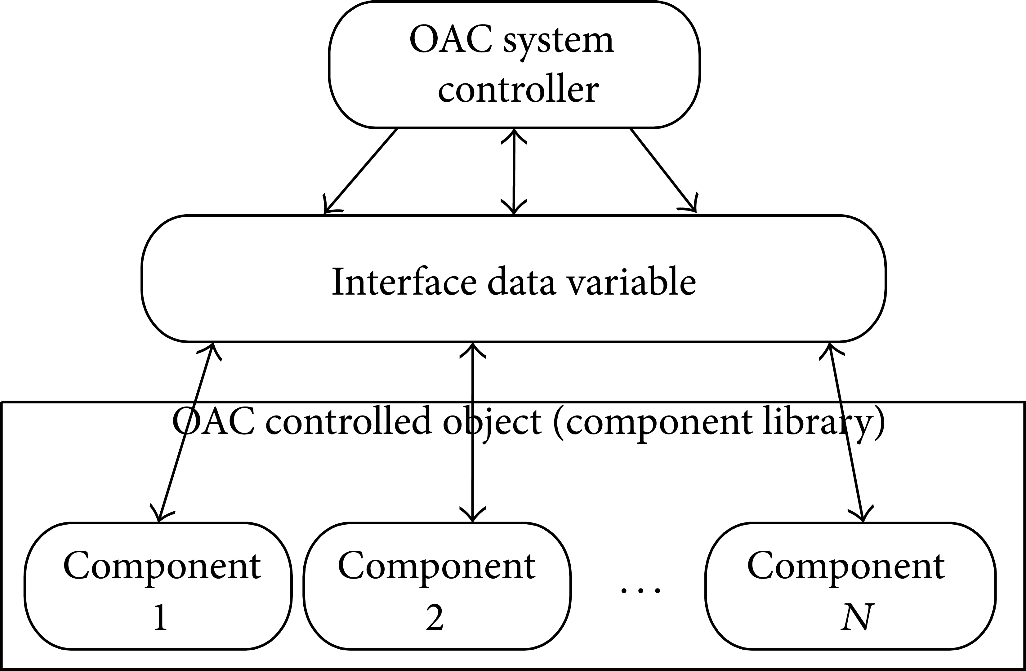
The structure of a typical OAC that consists of two parts: component library and system controller.

As shown in Figure 2, an OAC mainly consists of two main parts: a component library and an OAC system controller. The component library contains various components corresponding to different functions of a CNC. The OAC system controller is to configure, schedule, and cooperate components so as to make them work together to satisfy system requirements. To apply our closed-loop TTM model defined in Definition 9 (Section 3.2) on an OAC system, in which we define a closed-loop TTM as CT = (O,S,C), we have the following: the controlled object (“O”) is used to model the TTMs of the components of an OAC; the controller (“C”) is used to model the TTMs of the system controller of an OAC; the system specification (“S”) is used to model the system requirements in ATRTTL. Thus, after we obtain the TTMs of the components and system controller of an OAC, we can perform various verifications based on the system requirements described with ATRTTL.

Next, we give an exemplary component library in Table 3. Table 3 shows an exemplary component library that contains basic components for various functions of a CNC system. There are eight components: DEC (decoder), CTC (cutting tool compensator), INT (interpolator), PCTL (position controller), DSY (displayer), DET (detector), PLC (programmable logic controller), and SVO (position servo). The inputs and outputs of each component and its basic functions are shown in the table. For example, component DEC is the decoder that can decode an input NC (numeric control) program and generate Mcode and Gcode used for controlling machine cutting tools.

Table 3:

Components of OAC.

Based on the components of a component library, a system controller is used to combine the components and make them work together to provide system functions while satisfying system requirements. It has four main functions: configuration, scheduling, communication, and synchronization. Here, configuration means setting up the initial states of the components; scheduling means determining the execution sequences of the components; communication means passing information among the components; and synchronization means making the components work together with correct timing sequences. For example, as shown in Figure 3, a system controller can schedule the components and execute them following the given sequence. As the system controller is the key part of an OAC, we will analyze it in detail in Section 4.5.

Figure 3:

An expected execution sequence of an OAC.

4.3. The Component Library of OAC Systems

In this section, we specify the component library of an OAC system with our specification method at system level. In Section 4.3.1, we use the specification of the decode component as an example to show how to specify a component in our framework. In Section 4.3.2, in order to consider the relationship between different components, we add the environment TTM and the interface description to each component. In Section 4.3.3, we discuss how to specify the whole component library of the OAC system based on the individual component specification.

4.3.1. Specification of Components with TTM

In order to model the whole component library of OAC system, the first step is to model every component in component library. Next, we use the modeling of the decoder component (DEC) as an example to show how to specify a component with TTM. The TTM model of DEC is shown in Figure 4.

Figure 4:

The TTM model of the DEC component.

In Figure 4, a rectangle is used to represent a state and a directed edge between two states is used to represent one transition. Every transition contains four parts: the name, the lower and upper time bounds, the enable condition, and the transition function. For example, in the transition Reset[1|2](reset = true) → [reset_done:false], “Reset” is the transition name, [1|2] denotes the lower and upper time bounds, (reset = true) denotes the enable condition of the transition, and [reset_done:false] is the transition function. We attach “@” inside a state if it will be further specified in the model. For example, for “BUSY@,” we further specify state “BUSY” in Figure 5. This hierarchy structure can help simplify the modeling of a system.

Figure 5:

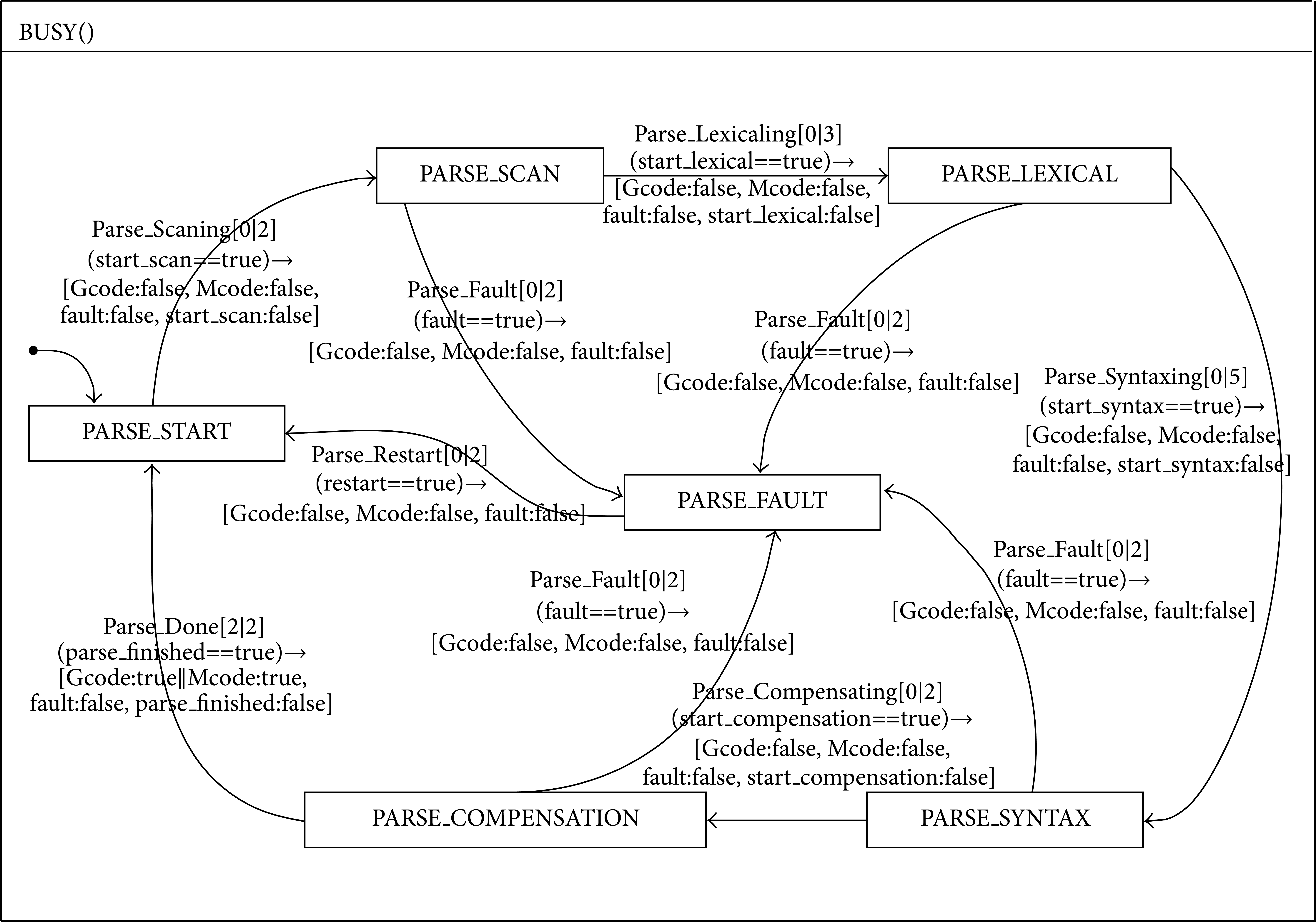
The TTM model of the DEC component at state “BUSY”.

From Figure 4, we can see that the open-loop behavior of DEC is separated into six states which are IDLE, BUSY, MCODE_DECODED, GCODE_DECODED, FAULT, and RESET. State IDLE represents that the decoder component is in a state waiting for a new NC -program segment to be inputted. State BUSY is the abstract description of the decoding procedure. “MDt” and “GDt” are used to represent the decoding time of one Mcode segment and that of Gcode segment, respectively. MCODE_DECODED and GCODE_DECODED are two states to represent that the decoding processes of Mcode and Gcode have been finished, respectively. State FAULT represents that an inputted NC-program segment is illegal. And state RESET represents that we need to reset the decoding component and restore its normal execution. The transitions of the whole decoding component are managed by the system controller.

As state “BUSY” is the most important phase for a decoder component, it is further specified in Figure 5. From Figure 5, we can see that there are six states, PARSE_START, PARSE_SCAN, PARSE_LEXICAL, PARSE_SYNTAX, PARSE_COMPENSATION, and PARSE_FAULT, in state “BUSY”. Among them, the first five states depict the normal procedure of a decoding scenario and the last one represents that there exists error. States PARSE_SCAN, PARSE_LEXICAL, PARSE_SYNTAX, and PARSE_COMPENSATION represent the main workflow of a decoder in “BUSY”; PARSE_SCAN is to separate the number, operator, and address word of one NC-program segment such as “G01 X10 Z10 F100”; PARSE_LEXICAL is to assign the number with the corresponding address word; PARSE_SYNTAX is to interpret the address word with a real specific engineering meaning; and PARSE_COMPENSATION is to change the result from state PARSE_SYNTAX to a format which a cutting tool compensator component (CTC) can recognize.

4.3.2. Constructing the TTM of Component Environment

Here we still use the DEC component as the example. As in Section 4.3.1, we can construct the TTM of component DEC without considering the interference of other components and the effect of system controller. In order to construct the component library TTM of OAC system, we should consider the relationship between other components in OAC with DEC. Here, we give the concept of environment TTM and add the interface description to TTM component.

Now we make the TTM component consisting of an interface specification and a body. The body is the TTM component which we already mentioned in Section 4.3.1. The purpose of the interface specification is to list all the shared variables or the message passing channels through which the component communicates with the outside. The shared variables in interface specification have three kinds of modes which are IN, OUT, and EXTERNAL. Mode IN means the variable in interface specification can be read in the body, mode OUT means the variable can be written in the body, and mode EXTERAL means the variable can be used by another component module. The interface specification can be described as a TTM environment. When finishing construction of all the component-environment pair of TTMs of every component, the component library TTM of OAC can be constructed. The DEC TTM component with its TTM environment is shown in Figure 6.

Figure 6:

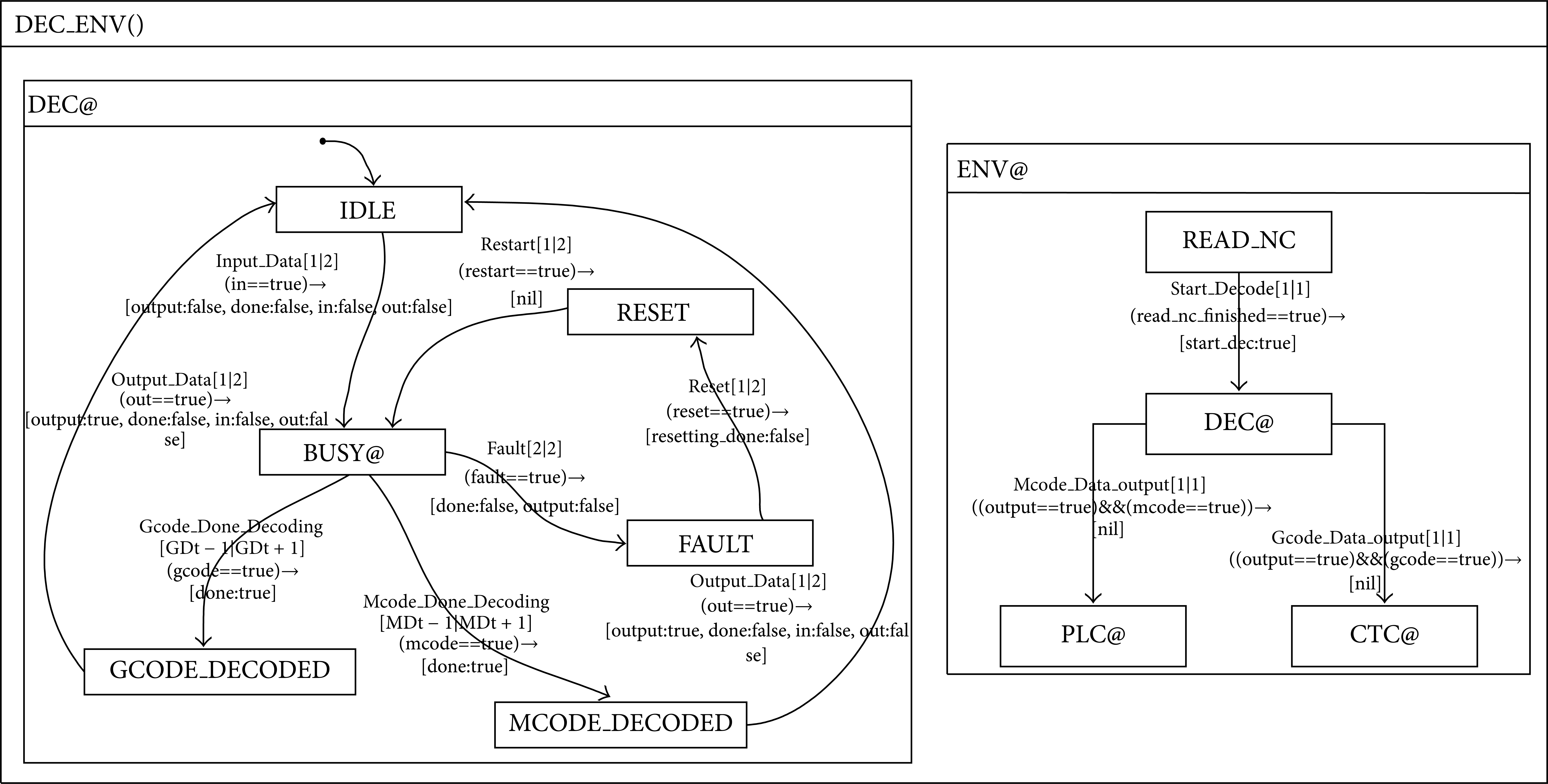
DEC component with its environment TTM ENV.

From Figure 6, we construct a new TTM component with two parallel composition TTMs DEC and ENV as

$\text{DEC}\_\text{ENV}=\left[\text{DEC}\parallel \text{ENV}\right].$

(27)

TTM DEC here is looked at as a body and TTM ENV is looked at as the interface specification of the body DEC. With the TTM ENV, we can restrict the model-checking procedure only to one component rather than the whole system. With this approach, we can effectively deal with the state explosion problem in Section 4.7.2. The ENV considers the interface variables through which the DEC component communicates with the outside. In Figure 6, we can see that the TTM ENV of DEC includes four interface variables: read_nc_finished, output, Mcode, and Gcode. Among them, read_nc_finished is declared to be mode of EXTERNAL IN and the other three variables are declared to be mode of EXTERNAL OUT.

4.3.3. The TTM Model of the Component Library of OAC Systems

After obtaining the TTM model of every component of an OAC system, we can construct a component library with the conjunction of the parallel compositions of the TTMs of components. From Definition 6, the TTM model of a whole component library can be obtained as follows:

$\begin{array}{c}\text{OAC}=\left[C_{\mathrm{1}}\parallel \cdots \parallel C_n\right]\hspace{0.5em}\hfill \\ \hspace{1em}=\left[\begin{array}{c}\text{DEC}\_\text{ENV}\parallel \mathrm{PLC}\_\text{ENV}\parallel \text{CTC}\_\text{ENV}\parallel \text{INT}\_\text{ENV}\parallel \hfill \\ \text{PCTL}\_\text{ENV}\parallel \text{SVO}\_\text{ENV}\parallel \text{DET}\_\text{ENV}\parallel \text{DSY}\_\text{ENV}\hfill \end{array}\right].\hfill \end{array}$

(28)

Note that the TTM model of a component library constructed above is only used to describe function modules of an OAC. To make the components work together to satisfy system requirements, a system controller is needed to configure, schedule, and cooperate components. Next, we will present how to describe the system requirements in ATRTTL in Section 4.4. In Section 4.5, we will show how to design and verify the system controller based on the TTM model of the component library and the system requirements described in ATRTTL.

4.4. The Specifications of System Requirements in ATRTTL

In the above section, we present how to model the component library of an OAC system. In this section, we present how to describe system requirements of an OAC in ATRTTL. The system requirements are the design goals of a system and they are specified by ATRTTL in this paper. After we obtain this set of specification with ATRTTL, we can perform verification to see if a system controller can satisfy the requirements.

In order to design reliable and dependable CNC systems, we specify six sets of system requirements in ATRTTFs as shown in Table 4: Future Liveness, Past Liveness, Safety, Fail-Safe, System-level Real-Time, and Component Real-Time.

Table 4:

Typical Specifications of an OAC in ATRTTL.

Future Liveness:
FL: ⫾(NC_code_Process_at_DEC → ⋄(Data_Process_at_CTC∨Data_Process_at_PLC))
Past Liveness:
PL: $\stackrel{-}{⫾}\left(\text{NC\_code\_Process\_at\_SVO}\to \stackrel{-}{\diamond }\left(\begin{array}{c}\text{NC\_code\_Process\_at\_PLC}\vee \\ \text{NC\_code\_Process\_at\_PCTL}\end{array}\right)\right)$
Safety:
S: ⫾(Data_Process_at_CTC → ¬Data_Process_at_PLC)
Fail-Safe:
FS: ⫾(fault_in_C → ((⋄¬C_normal)UReset_C)) Here, C = DEC, PLC, CTC, INT, PCTL, SVO, DET, DSYand ¬C_normal = C in a FAULT state and Reset_C = C in a RESET state
System-level Real-Time:
ST:⫾((NC_program_Input∧mocde = true) → ${\diamond }_{\begin{array}{c}[\text{MinDecTime+MinPlcTime+MinSvoTime+MinDsyTime,}\\ \text{MaxDecTime+MaxPlcTime+MaxSvoTime+MaxDsyTime}\end{array}}\text{DSY\_Finished}$
Component Real-Time:
CT: $⫾\left(\text{Start\_Process\_at\_DEC}\to {\diamond }_{[\text{MinDecTime,MaxDecTime}]}\text{End\_Process\_at\_DEC}\right)$

In Table 4, “Liveness” is known as the “good” things that should happen, which partially determines the reliability and dependability of a system. For an OAC, it means that the system should work on right time sequences. There are two categories of liveness property which are Future Liveness and Past Liveness so we can verify events in the past and future. For ATRTTF FL, it means when the NC code has finished processing in component DEC, it should then be processed in component CTC or component PLC. For ATRTTF PL, it means when the NC code is now being processed in component SVO, it should just have gotten the data either from component PLC or from component PCTL.

“Safety” is known as the “bad” things that should not happen, which determines the safety of a system. For S, it means the data of one single NC-program segment cannot be processed in CTC component and PLC component simultaneously.

“Fail-Safe” is used to deal with the conditions when mistakes occur, which relates to reliability, dependability, and safety. For FS, it means that when there are some problems in any component, the component cannot restart to work until this component returns to the RESET state.

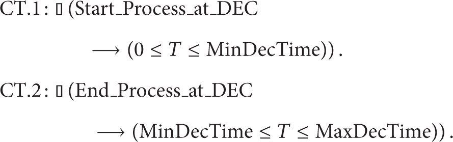
“Real-Time” means that a certain event (state) must happen in a specified time interval. Real-Time specification is important for CNC systems since it may cause disaster if a real-time event cannot be finished within its deadline. For ST, it means when the OAC system starts to work, it must finish all the functions in the time interval between MinDecTime + MinPlcTime + MinSvoTime + MinDsyTime and MaxDecTime + MaxPlcTime + MaxSvoTime + MaxDsyTime. For CT, it means when the component DEC starts to work, it must be finished in the time interval between MinDecTime and MaxDecTime.

In Sections 4.5 and 4.6, we will give the analysis and verification results of the above six categories of functional ATRTTL formula.

4.5. Design of OAC System Controller

Based on the results of the library component in Section 4.3 and the system specifications of an OAC in Section 4.4, in this section, we design a system controller so that the library component can work under it in the manner of what the specifications of OAC require. System controller is the most important part in OACs, and it cooperates, synchronizes, and makes all the components work together to satisfy system requirements that represent as the ATRTTFs based on our TTM/ATRTTL specification method. In Algorithm 1, we show an integrated procedure to design a system controller of an OAC. Basically, the whole procedure of designing an OAC system controller has three main steps. The first step is to construct the open-loop component library TTM of OAC system, which is already depicted in Section 4.3. The second step is to express the whole OAC system requirement specifications, which is already given in Section 4.4. The third step is to present the sound system controller which we will give in detail in this section.

Algorithm 1:

The procedure of designing the system controller.

4.5.1. Constructing the TTM of Component Controller

From Step 8, the system controller C is constructed based on component controller C _i in a hierarchical manner using the bottom-up approach. Using this method, we can construct or analyze a complicated system controller by a relatively simple component controller. So first in Step 7, we should give the component controller of every component TTM. Here, we still use the DEC component as the example seen in Figure 7.

Figure 7:

DEC component controller TTM.

From Figure 7, the controlling way of TTM DEC_CONTOLLER on DEC_ENV is as follows: by accepting the ENV command start_dec, the DEC_CONTROLLER begins to work and issues the command in to the DEC. Then the DEC starts to work until the decoding procedure is completed by issuing a flag variable done. When the DEC_CONTOLLER receives done, it issues a flag out to DEC and gives the value to Gcode or Mcode to decide whether the NC-program segment is a logic order to PLC or an interpolation order to CTC. By receiving these three flags, the DEC runs on a right way and is ready to decode a new segment. If the input NC-program segment is wrong in expression by receiving false value of flag done, the DEC_CONTROLLER will enter into the MCODE_FAULT state or GCODE_FAULT state based on the kind of segment and in the same time will issue the reset flag to start the reset procedure. The procedure is finished and issues the resetting_done flag. By receiving this flag, the DEC_CONTROLLER moves the state to DECODNG and decodes a new NC-program segment. With the parallel combination of the TTM DEC_ENV and TTM DEC_CONTROLLER, a closed-loop TTM of DEC is constructed and can be analyzed individually.

4.5.2. Constructing the System Controller C of OAC

In this step, the variable set, the sequence of loading components, the communication between components and starting the whole OAC system are controlled by the given system controller. The procedure of designing a system controller is constructed in a hierarchical manner using a bottom-up approach [2, 31]. Based on the results of Section 4.5.1, we can give an initial guess of system controller of the whole OAC system in Step 8 of Algorithm 1. The procedure of guessing is to construct a system controller in TTM which coordinates all the actions of each closed-loop component TTM.

The actions of each closed-loop component are expressed by the interface variables. The interface variables only preserve the function and connection with other components or the OAC system and encapsulate the detail of the components. So when dealing with the whole OAC system, we only face the reduced complexity interface of components which only preserve the sufficient information of designing the system controller of OAC.

In Section 4.3.2, we have already given the concepts of environment and interface variable and its modes. The environment includes all the information of the relationship with the outside and the number of interface variables determines the coupling level of component. The EXTERNAL IN variable is used to get the information from the other components or the system controller and the EXTERNAL OUT variable is used to issue the results of component to the outside. For the DEC component example, it reads the flag variable read_nc_finished to start the process and finishes the process by issuing output, Mcode, and Gcode. These four interface variables include all the information about the component DEC with the outside. So we can only consider these kinds of variables when we design the system controller C of OAC.

When we get all the interface variables of all the components, the next work is guessing a reasonable controller C in Step 8 of Algorithm 1. We should consider both the information of all the closed-loop components and the system-level functional property specifications in ATRTTL which we have already presented in Table 4. Although we can use the bottom-up method to give an initial guess of system controller from the relatively simple component TTM in a modular way, we still need a great deal of insights of designer to give a sound process sequence which determines the work load of the whole design procedure. When we get the initial guess of controller, the next step is to verify the controller using an iterative way in Step 9. We modify the controller by adding or replacing the interface variables for different states of system. The iterative procedure is finished when all the property specifications are verified.

In the following, an example is given to design a system controller for a typical NC-program segment in a two-axis OAC system. The program segment is SEGMENT: G01 X10.0 Z10.0 M05 F1000.0. This SEGMENT is a line-interpolation procedure from the start point (0, 0) to the end point (10.0, 10.0) and the velocity of interpolation is 1000.0 mm/min. When finishing interpolation, the spindle is shut.

Based on the above NC-program segment, we carry out a reasonable processing flow to control the action of OAC system. The guess of initial system controller perhaps is obviously wrong at the early stage and will become more and more precise under the iterative simulation of the system controller. Based on this idea, we can firstly give a relatively sound initial OAC system controller based on the TTM of every component in Figure 8.

Figure 8:

The system controller TTM of OAC.

4.5.3. Modifying the System Controller C with Verification Tools

In Section 4.5.2, we have already presented a reasonable guess of system controller to the greatest extent, but we still need a formal way to prove that the controller is right and if it has flaws and to know how to find it and correct it in a sound way. The verification tool should be used to analyze and verify the given ATRTTFs. If the given system controller can satisfy the specification of closed-loop OAC [P∥C], then the verification tool can give an answer “yes” with outputting the number of states explored. If the verification tool finds an error in the system controller, it will give out a counter-example explaining in which state of the system controller TTM exists a flaw and based on this information we can modify the controller to reach the specification of the closed-loop OAC in ATRTTL and iteratively compute this procedure until all the specifications can be satisfied using the modified controller. The procedure is shown in Step 9 and Step 10 in Algorithm 1.

4.6. Design of Scheduling Mechanism of OAC

From Sections 4.3 and 4.5, we have constructed a typical closed-loop OAC system in TTM. By this model, we can deal with the functional properties and time properties in some conditions. But the system controller only gives a sound but idealized controlling sequence. In reality, in order to analyze and verify real-time properties, we should introduce the scheduling mechanism into the OAC closed-loop system and based on it we then can get the real-time checking results in a proper way. In this section, we first give the whole structure of the modified OAC system. Based on it, we will then model the scheduling mechanism in TTM. In the last part, we will present the TTM model of the message passing mechanism which is the standard communication method in asynchronous event driven system.

4.6.1. OAC TTM with Scheduling Mechanism

The new OAC TTM with scheduling mechanism includes three concurrent component TTM modules. One is called OAC_with_Scheduler. It includes several OAC processes and a system-level scheduler. Every process represents a single component in OAC. Since at any time only one process is permitted to run, the scheduler is used to determine the execution of time sequence. The second concurrent is hardware interrupt. It is used to simulate the hardware timer which generates the time-out instruction in every constant time interval. The third part is the process FIFO queue. It follows the first-in-first-out strategy and it is used to help the scheduler to deal with the scheduling task. The detail of these three concurrent TTMs is explained later. The whole structured OAC system with scheduling mechanism is shown in Figure 9.

Figure 9:

System-level OAC TTM with OS TTM.

4.6.2. Scheduling Mechanism and FIFO Queue

The whole scheduling mechanism can be depicted as follows. When any component process is ready to be executed, it will write its ID in FIFO queue and wait to be permitted to run. The permission command is achieved from the scheduler. The scheduler itself is permitted to run under the command of hardware interrupt. The hardware interrupt issues the start_running_scheduler command every constant time interval IT < T < IT + 1. On receiving the start_running_scheduler command, the scheduler will get the process ID from the top of FIFO queue and this process will be executed immediately.

The TTM of scheduler is shown in Figure 10. It depicts the procedure of getting the process ID from FIFO queue and the update operation of the queue.

Figure 10:

TTM model of OAC scheduler.

Writing the process ID to FIFO mechanism is shown in Figure 11. We can see if the ID already exists in FIFO, then the writing ID to FIFO operation is canceled.

Figure 11:

TTM model of FIFO queue.

4.6.3. Message Passing Mechanism

The communication between different processes is executed by a message passing mechanism. It follows in several steps below.

In transmitting end, first, because of an occurrence of a transition in process, a variable is changed by this transition. Then, the message corresponding to this changed variable is set to be TRUE in a constant time interval Ttime. In receiving end, first, this changed message is received and decoded. If the information of this message is TRUE, then the variable corresponding to this message is also set to be TRUE after a constant time interval Rtime. In the last, the message is reset to be FALSE in a constant time interval Itime in order to be used in the next time.

The TTM of message passing mechanism is shown in Figure 12.

Figure 12:

TTM model of message passing mechanism.

4.7. Verifying System-Level Specification with ATRTTL

4.7.1. Overview of Formal Verification Method

In our formal verification method, we choose two toolsets to be used which are STeP by Stanford Temporal Prover group and SF2STeP by D. Lalita.

STeP is a system being developed to support the computer-aided analysis and verification of many kinds of system such as concurrent system, reactive system, and real-time system. The analysis and verification process is for the most automatic part. It encapsulates many tools and methods such as efficient simplification methods, decision procedures, and invariant generation techniques so we can directly use this toolset without concerning the details of verification procedure.

The inputs of the STeP toolset are temporal logic formula and fair transition system. So there is a gap between our TTM/ATRTTL model and the inputs of the STeP. We should find an effective way to translate the TTM/ATRTTL model to a form which the STeP can recognize.

Before verifying the OAC system using STeP, we use another toolset SF2STeP. SF2STeP allows converting a generic Stateflow diagram to a timed Stateflow diagram and also can translate the timed Stateflow diagram to a fair transition system. Then with the fair transition system and the temporal logic in ATRTTL, we can then use the STeP toolset.

The flow chart of the whole verification procedure is shown in Figure 13.

Figure 13:

Verification procedure of OAC.

The whole procedure of verification is used to ensure all states of the system are correct and all time sequences are sound.

4.7.2. Some Analysis and Verification Problems through Simulation in STeP

(1) Rewrite Rules. Because the STeP cannot directly process the formulas with binding operators, the real-time specification in ATRTTL cannot be verified in the straight way. So we need the rewrite rules to change these kinds of formulas with binding operators to a relatively simple one with only one temporal operator.

For example, let us consider the specification CT. let SDt represent the start time of component DEC and let EDt represent the finished time of component DEC; then we can rewrite the ATRTTF into the following equation as

$\text{CT}:▯(\left(\left(\text{EDt}-\text{SDt}\right)\ge \text{MinDecTime}\right)\wedge \left(\left(\text{EDt}-\text{SDt}\right)\le \text{MaxDecTime}\right)).$

(29)

Furthermore, in order to further simplify the real-time property ATRTTL equation form, we now only consider a global time variable T as the measure standard. We consider that the times of events in Table 4 are all measured relative to the start time point. We can change (29) into a pair of equations as follows:

$\begin{array}{c}\text{CT}.\mathrm{1}:▯(\text{Start}\_\text{Process}\_\text{at}\_\text{DEC}⟶\left(\mathrm{0}\le T\le \text{MinDecTime}\right)).\hfill \\ \text{CT}.\mathrm{2}:▯(\text{End}\_\text{Process}\_\text{at}\_\text{DEC}⟶\left(\text{MinDecTime}\le T\le \text{MaxDecTime}\right)).\hfill \end{array}$

(30)

Equation (30) is equivalent with (29). In (30), there is only one variable T to analyze. With this easy form of ATRTTL formula, the real-time properties can be verified into the STeP.

(2) Verification Rules. Based on Definition 8, we can give a simple verification rule which can be used in simplifying the ATRTTL formula of OAC. The most important feature of verification rules is that it can convert a given temporal logic formula.

With Rule 1 (INV), we can only check the verification condition of formula φ. Since the only transition which can influence the real-time properties is the tick transition, we now reduce the original real-time ATRTTL formulas in Table 4 to only prove the verification condition of tick transition. Then the model-checking procedure becomes easier to control.

(3) State Explosion Problem. When dealing with real-time properties, the tick transition happens infinitely often so the exploration of states will eventually occur. There are two methods to deal with the state explosion problem. The first one is reduction to absurdity by $(A\to B)\iff (\stackrel{-}{B}\to \stackrel{-}{A})$ . Basically if we want to prove the validity of a real-time ATRTTL specification in a normal way to model-check each state in TTM using STeP; we can give a contrary specification of the original one and prove it by contradiction.

The second method to deal with the explosion is modular verification. For the whole CNC system, the number of states is very big. For example, when dealing with the specification such as component real-time CT in Table 4, we only need to focus on the states which are relevant to DEC component without concerning other components and system controller based on the ENV of DEC. Using this method, we can dramatically reduce the number of states.

(4) Time Bound Restriction. Since our OAC system is a typical loop executing system, when dealing with the complicated property ATRTTL such as ST, we can only verify it in a single loop; that is to say, we add another enable condition to every transition in whole OAC system. This enable condition restricts the global T variable at the value of one cycle of operation. By this method, we can further lower the number of states to enumerate.

4.7.3. Experiments for Verifying an OAC System

(1) Dead Lock. In our TTM of OAC system, the dead lock is generated from the scheduling and the message passing strategy we have already mentioned in Section 4.6. The origin of this problem is because of the uncertainty of the logical control pattern of OAC system. In order to show the dead-lock problem more clearly, a counter example which is generated by model-checking tool of STeP is shown.

From Table 5, we can see when the whole system wants to schedule the SVO process to operate, it first makes the process C become active and at that time the process PCTL and process PLC give the system-level controller message PCTL_Finished and PLC_Finished, respectively. But because process C gets these two input messages at the same time, the behavior of C is not predictable on sending the output message to PCTL process or PLC process or both. If any of these two processes is ignored by C, then a dead lock is reached because the system controller C and any one of these two processes will wait for each other on input message commands.

Table 5:

Example of event sequence of dead lock.

Time	Event
0.01	Start_running_controller
0.02	Start_Decode_Segment
0.05	Message [C2DEC] = 1
⋮	⋮
87.23	Start_running_controller
87.28	PCTL_Finished
87.28	PLC_Finished
87.28	Begin_SVO_Gcode
87.28	Ignoring Begin_SVO_Mcode
87.32	Message [PLC2C] = 0
87.32	Message [C2PCTL] = 1
87.32	Message [PCTL2C] = 0
87.32	Ignoring Message [C2PLC] = 1
88.14	Start_running_scheduler
88.15	reading_FIFO
⋮	⋮

This problem can be easily solved by changing the scheduling pattern of Figure 10. Before every cycle of routine scheduling task begins to run, we first check whether the system controller process C is in the FIFO queue. If it is, we will then move C to the top of the FIFO; that is to say, since we give the system controller the highest priority, the undetermination of C can be avoided and, at any time, C can only serve one other parallel process. The improved TTM model of OAC scheduler is shown in Figure 14.

Figure 14:

Improved TTM model of OAC scheduler.

(2) Component Time Bound Checking. When we use the model-checking tool of STeP to verify the ATRTTL real-time property ST, we find that not all the computations can satisfy the closed-loop OAC system and that the verification procedure reaches a counter example of dead loop of tick. But if we change the original time parameter-upper bound of PLC 20 to a new value 35, then the model-check procedure is complete. It means even though the logic relationship of the execution sequence is correct, the unsuiTable value of time parameters can also have an effect on the OAC system. Based on this verification procedure, we can determine the permissible time bound of each component of OAC without concerning the detail before the development of the real system. This method is helpful for designer because the change of design at the beginning of development will cost less compared to the latter procedures. In our verification result from STeP, we can get the appropriate time parameters of all components which are shown in Table 6. The time bound is not the real OAC system time bound; it only gives the proportion relationship of time values between different processes.

Table 6:

Correct time parameters of components (microsecond).

Component	Lower time bound	Upper time bound
DEC	10	20
PLC	10	35
CTC	10	20
INT	10	20
PCTL	10	20
SVO	10	20
DET	5	10
DSY	20	30

(3) Verification Results Using STeP. The verification results of specifications using STeP are shown in Table 7. The consuming time and the number of states explored are given in Table 7. From Table 7, since all the six categories of OAC specifications are satisfied and no counter-example state exists, we can draw the conclusion that the OAC library component can work under the system controller in the manner of what the specifications of OAC require. The designed component library and the system controller of closed-loop OAC system are correct.

Table 7:

Verification results of functional specifications.

Functional specification	Number of states explored	Consuming time (secs)
FL	23323	84
PL	25445	92
S	29986	34
FS (modularized)	330	1
ST (rewritten)	23988	12
CT (rewritten)	2453	2

5. Conclusion and Future Work

In this paper, we proposed a new modeling method called TTM/ATRTTL (timed transition models/all-time real-time temporal logics) for specifying CNC systems based on TTM/RTTL. TTM/ATRTTL provides full support for specifying hard real time and feedback that are needed for modeling CNC systems. We also proposed a verification framework with verification rules and theorems and implemented it with STeP and SF2STeP. The proposed verification framework can check reliability, safety, and correctness of systems specified by our TTM/ATRTTL method. We applied our modeling and verification techniques on an open architecture CNC system and conducted comprehensive studies on modeling and verifying a system controller that is the key part of an OAC system.

The results show that our method can effectively model and verify OAC systems and generate OAC software that can satisfy system requirements in reliability, dependability, and safety.

In the future, we will investigate how to integrate our TTM/ATRTTL technique into real-time systems so we can generate reliable and dependable system software for CNC systems with our specification and verification methods. We will also study how to translate TTM/ATRTTL specifications into hardware description language such as VerilogHDL so we can directly implement a CNC control system with FPGA.

Conflict of Interests

The author declares that there is no conflict of interests regarding the publication of this paper.