Modeling the Speed Choice Behaviors of Drivers on Mountainous Roads with Complicated Shapes

Abstract

Roadway geometric features and pavement conditions can significantly affect driver behavior, particularly with regard to vehicle speed. This paper presents the development of an algorithm for speed selection for use in automated passenger car travel (without driver input) on mountainous roads with complicated shapes. The relationship between favorable driving speed and the geometric features of horizontal curves was established on the basis of driving experiments and spot speed observation data, and speed control models were established for driving on curves, curve approaches/departures, and tangents. The models developed can be used to calculate a driver's desired speed on any roadway with a defined geometry. The model considers the driver's behavior type and the vehicle's dynamic properties. This paper presents the results of simulation experiments on roads with small curve radii and narrow widths. The algorithms developed may be used for assisted and automated driving. Under automated driving conditions, speed control and speed change based on the algorithms developed make drivers feel natural as if they drive the car themselves.

1. Introduction

To achieve safe automated travel by passenger cars on roads, two types of operations are required: rotating the steering wheel to ensure that the vehicle is pointed in the expected direction and braking/accelerating to control the speed within the expected range [1]. A rational desired path and desired speed should thus be determined before the correct controlling operation is initialized. Therefore, modeling the driver's speed choice to determine the target speed for a passenger car is one of the two major requirements [2].

For cars driving on urban streets or heavy-duty vehicles following the trucks in front, the primary task in speed control is to maintain a safe distance and avoid conflict with other vehicles. In these situations, the controlling factor in the desired driving speed is the headway, not any of the roadway geometry features. Driving on expressways is a similar situation because the critical safety speed controlled by the minimum curve radii used in alignment design (approximately 400–500 m) exceeds the highest cruising speed published in existing researches; that is, roadway geometry has little effect on speed control [3–5].

The situation is very different when a vehicle is traveling on lower-standard rural roads in mountainous areas where, to fit the topography, the alignments are complex, with frequent curvature changes. The geometric features of such roads have a substantial influence on the speed choice, and drivers must frequently adjust their driving speeds to ensure the lateral and longitudinal stability of their vehicles. According to Polus et al. [6], drivers on tangents should choose lower speeds on narrower roadways and higher speeds on wider roadways. Lamm and Choueiri [7] specified a fixed acceleration or deceleration rate to describe the speed changes that occur when a car enters and exits a curve. The radius of curvature is the geometric feature used to determine the speed at which a curve is negotiated [8].

The driving width (i.e., the pavement width used by drivers) can play a role in the tangent speed and has an important effect on the driving speed during entry into a sharp curve. A greater speed reduction is needed to enter a sharp curve safely rather than to enter a flat curve, so a more powerful braking needs to be applied. The deflection angle of a curve can obviously change the driving speed, but almost all existing speed prediction models fail to consider the influence of the deflection angle and driving width on speed choice of curve negotiation [9]. If these speed models are applied to automated driving (using adaptive cruise control) on roads with complicated shapes, the speed adjustments made in curved areas will not be flexible enough to simulate the real reactions of drivers, and the result is that drivers may feel discomfort. Sentouh et al. [10] proposed an algorithm to determine the critical safety speed: if the driving speed exceeds the upper bound of a speed profile, an alarm is triggered to warn the driver, so the speed profile can work as the upper limit of the driving speed rather than the target speed.

This paper presents a model for the speed control behavior of a passenger car driver as a function of the geometric features of roads. For passenger cars, the geometric features of horizontal curves, such as the curve radii, road widths, lane widths, deflection angles, and the use of emergency lanes, play a more important role in speed choice than the longitudinal grade. In contrast, the longitudinal grade may play a more important role in the speed choices of drivers of freight vehicles. The desired speed profiles along a roadway can be determined using the models described in this paper. These desired speed profiles can be used as target speeds for passenger cars and thus be employed in intelligent driver support systems and advanced driver assistance systems.

2. Driver's Speed Choice on Curves

2.1. Influence of Curve Radius on Speed Choice

Any driver—regardless of experience, age, or gender—will reduce the speed of a vehicle when entering curves with small radii (sharp curves). Experience teaches drivers that they will suffer discomfort resulting from centrifugal force and the potential for a vehicle rollover toward the outside of the curve. Therefore, the keys to speed choice and adjustment are establishing a sense of safety when drivers drive their cars for, maintaining control of the roll angle of the vehicle caused by lateral force, and ensuring that the vehicle responds as expected to the steering input. These driver perceptions associated with the driving speed can be described in terms of the lateral acceleration a _y [11, 12]. Therefore, a _y can be used as a physiological measure of the safety of a driver on a curve. In this study, the lateral acceleration tolerated by a driver is defined as a_{y, tol}. When a _y > a_{y, tol}, the driver will subconsciously sense that the vehicle's driving conditions are unsafe and may be out of control. To avoid such risks, the driver will reduce the speed, which results in a _y ≤ a_{y, tol}. Therefore, a_{y, tol} can be used to determine the desired speed on curves.

To determine the relationship between a_{y, tol} and the curve radius R, operating speeds on curves were measured on two rural roads. The first was a tertiary rural road with a design speed of 40 km/h, two 3.5 m wide lanes, and a 0.3 m wide paved shoulder on each side. The second was a fourth-class road with a design speed of 20 km/h, one 3.5 m wide lane, and a 0.25 m wide paved shoulder on each side. A Newcon speed detector (Newcon Optik, Toronto, Ontario, Canada) was used to measure the speeds of passenger cars near the midpoints of curves on these two roads. The speed data and curve radii were used to calculate the lateral accelerations a _yi of each observed car with respect to the curve radii, as shown in Figure 1. There was a clear negative relationship between lateral acceleration and curve radius R. The following model was developed for a_{y, tol} as a function of R:

$a_{y,\text{tol}}={\beta }_{\mathrm{1}}+\frac{{\beta }_{\mathrm{2}}}{R^h+{\beta }_{\mathrm{3}}},$

(1)

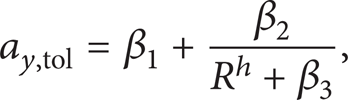
where β₁–β₃ and h are parameters used to determine the shape of the curve of a_{y, tol} versus R.

Figure 1:

a _y of passenger cars versus curve radius: (a) measured on a tertiary rural road; (b) measured on a fourth-class rural road.

If a_{y, tol} is to represent an average for all drivers observed, all of the a _yi data should be used to calibrate the regression coefficients. If a_{y, tol} is to represent drivers who prefer higher speeds, only the 85th percentile of the lateral accelerations should be considered.

Driving speed is closely related to the horizontal, vertical, and cross-sectional design elements of a road because these geometric attributes result in various speed choice behaviors [13]. For instance, if a driver enters a curve with a radius of 400 m on a two-lane highway at a speed of 40 km/h, he or she will typically not slow down and may even accelerate the vehicle. However, if the driver enters a curve of the same radius on a four- or six-lane expressway at a higher speed, he or she will obviously slow down because a 400 m curve radius is the sharpest design curve radius allowed for such roadways. Thus, the model parameters need to be calibrated separately for the two different road types. Based on experimental and observation data collected on 12 roadways (eight two-lane highways and four expressways), the values of the parameters in the model shown above are β₁ = 0.25, β₂ = 5000, β₃ = 1380, and h = 1.335 for expressways with 4–6 lanes and β₁ = 0.3, β₂ = 3500, β₃ = 1850, and h = 1.22 for two-lane roads.

2.2. Influence of Lane Width of Curved Segment on Speed Choice

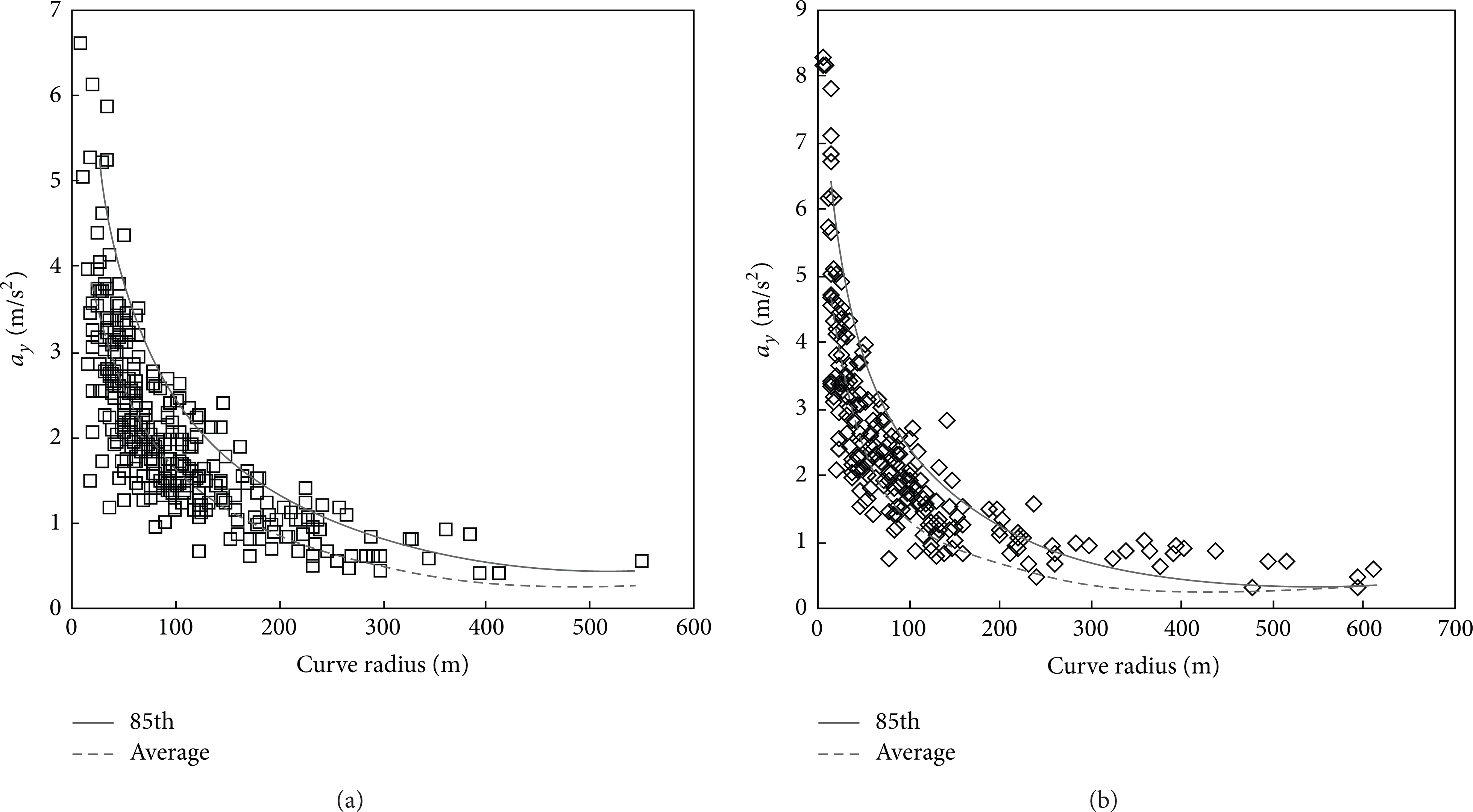
The data collected on driving behavior revealed that the driving lane width W_DL has a clear influence on the speed choice. For a given curve radius, a wider lane permits a greater driving speed and vice versa. The reason for this is that a greater W_DL makes “corner-cutting” effectiveness of a driver's desired path easier [14]. Consequently, the desired path can pass closer to the inside of the curve, resulting in a straighter trajectory (see Figure 2). Drivers speed up subconsciously in such situations. The influence of W_DL on “corner-cutting” effectiveness also depends on the curve radius. A smaller R means that a larger corner can be cut and the driver can increase the speed more.

Figure 2:

Effect of driving width on track curvature: (a) 4 m width, following the curve; (b) 4 m width, cutting the curve; (c) 6 m width, cutting the curve; (d) 10.5 m width, cutting the curve.

The driving lane width W_DL is usually 3.0–3.75 m. However, lower-standard roads in mountainous areas can have lanes as narrow as 2.4 m. In contrast, lanes on secondary highways can have widths of 7 m or more if an emergency lane is added. Therefore, in this study, a range of 2.4–7 m was considered for W_DL. To determine the effect of W_DL on drivers' speed choice behaviors, vehicle speeds at the midpoints of curves on eight rural roads of various lane widths were measured. Curves with similar deflection angles were gathered in the same group to isolate the influence of curve deflection angle. In each group, the variation in curve radius was less than 10 m. Approximately 15–20 passenger car speeds were recorded for each curve, and the arithmetic mean of the speeds for that curve was determined. For example, Figure 3(a) shows the average speeds observed on a group of curves with radii of approximately 45 m. For modeling convenience, an equivalent radius R _e , illustrated in Figure 2, was defined as follows:

$R_e=\frac{V_c^2}{a_{y,\text{tol},R_i}},$

(2)

where $a_{y,\text{tol},R_i}$ is the corresponding tolerable lateral acceleration when R = R _i and R _e is the radius of the vehicle trajectory at the midpoint of a curve, which increases with the width of the driving lane because drivers can use more space to cut the curve (see Figure 2). Thus, R _e /R can be used to describe the effect of lane width on the speed choice on curves. That is, R _e is used instead of R to calculate the curve negotiation speed V _c if the influence of the lane width is considered.

Figure 3:

(a)–(i) Positive relationship between R _e /R and driving lane width; (j) influence of curve radius on R _e /R; (k) three-dimensional representation of λ _w .

The speeds measured at the midpoints of the curves were substituted into (2) to obtain R _e /R for all of the curves considered. The results, shown in Figure 3, indicate that decreasing the curve radius increases the effect of the lane width on the equivalent radius. Therefore, the effect of the curve radius can be expressed in the model by a width influence coefficient λ _w . Two secondary influence factors, λ_w1 and λ_w2, were defined to express the effects of the lane width and curve radius, respectively. The regression formula

${\lambda }_{w\mathrm{1}}=\mathrm{0.0872}{W}_{\text{DL}}+\mathrm{0.7205},$

(3)

which corresponds to the curve with a radius of 110 m, was chosen as the model for λ_w1. Because R _e /R is linear with respect to the lane width for all test groups λ_w2i, discrete values of λ_w2, calculated from the equation

${\lambda }_{w\mathrm{2}i}=\frac{\left({\left.\left(R_{ei}/R_i\right)\right|}_{W_{\text{DL}}=\mathrm{7}}\right)}{\left({\left.\left(R_{ei}/R_i\right)\right|}_{W_{\text{DL}}=\mathrm{7},R_i=\mathrm{110}}\right)},$

(4)

reflect the influence of the curve radius. The data in Figure 3(j) indicate a strong negative correlation between λ_w2i and R. The following regression equation for λ_w2 as a function of R was obtained:

${\lambda }_{w\mathrm{2}}={\left(\mathrm{0.6871}+\frac{\mathrm{489.7261}}{\mathrm{12.2910}R-\mathrm{11.8359}}\right)}^{\mathrm{1.5}}.$

(5)

The final model for λ _w , expressing the effects of both the lane width W_DL and the curve radius R, is as follows:

${\lambda }_w=\left\{\begin{array}{cc}\mathrm{1}+\left({\lambda }_{w\mathrm{1}}-\mathrm{1}\right){\lambda }_{w\mathrm{2}},\hfill & \text{if}\mathrm{\hspace{0.17em}\hspace{0.17em}}{\lambda }_{w\mathrm{1}}\ge \mathrm{1}\hfill \\ \mathrm{1}-\left(\mathrm{1}-{\lambda }_{w\mathrm{1}}\right){\lambda }_{w\mathrm{2}},\hfill & \text{if}\mathrm{\hspace{0.17em}\hspace{0.17em}}{\lambda }_{w\mathrm{1}}<\mathrm{1}.\hfill \end{array}\right.$

(6)

A three-dimensional representation of λ _w with respect to W_DL and R is plotted in Figure 3(k).

2.3. Influence of Curve Deflection Angle on Speed Choice

To model the effect of the deflection angle on speed choice, the driving speeds of passenger cars were measured at the midpoints of curves on four rural roads. The curves had similar lane widths of 3.5–3.75 m and similar paved shoulder widths of 0.5–0.8 m; therefore the influences of lane width and pavement width were minimized. Figure 4(a) shows ΔV _c , which is the residual speed calculated from the curve negotiation speed V _c minus the speed corresponding to the maximum deflection angle, plotted against the deflection angle. This residual speed parameter is calculated so that profiles for different curve radii can be shown together in one coordinate system. This figure indicates that increasing the deflection angle results in a decrease in driving speed. The curve radius influences this effect: a smaller curve radius increases the effect of the deflection angle on the driving speed.

Figure 4:

Effect of increase in curve deflection angle.

Because the parameters used to calculate the desired speed on curves are a_{y, tol} and R, the influence of the deflection angle on speed must establish direct connection with one of the two parameters. In this study, R was used to reflect that influence. Figure 4(b) shows curves of R _e /R versus the deflection angle, where R _e is defined as in Section 2.2. The deflection angle influence coefficient λ_ΔA is modeled in a manner similar to that for λ _w . In other words, two secondary influence coefficients, λ_ΔA1 and λ_ΔA2, were defined to reflect the effects of the deflection angle and curve radius, respectively.

As Figures 4(a) and 4(b) show, the speed is only reduced when ΔA is below a critical deflection angle ΔA_cr. Therefore, the first step is to determine the value of ΔA_cr for a given curve. The linear regression formula

$\Delta A_{\text{cr}}=\mathrm{84}-\mathrm{0.106}R$

(7)

was obtained for the negative correlation between ΔA_cr and R (see Figure 4(c)). The next step was modeling the change in R _e /R with respect to ΔA. Data for R _e /R corresponding to a 160 m curve radius were used to determine λ_ΔA1. For comparison, an inverse function with a better fit was selected as the model for λ_ΔA1:

${\lambda }_{\Delta A\mathrm{1}}=\left\{\begin{array}{cc}{\left(\frac{\mathrm{0.45}(\Delta A_{\text{cr}}+\mathrm{15})}{\Delta A-\mathrm{6}}\right)}^{\mathrm{0.3}}+\mathrm{0.125},\hfill & \text{if}\mathrm{\hspace{0.17em}\hspace{0.17em}}\Delta A<\Delta A_{\text{cr}}\hfill \\ {\left(\frac{\mathrm{0.45}(\Delta A_{\text{cr}}+\mathrm{15})}{\Delta A_{\text{cr}}-\mathrm{6}}\right)}^{\mathrm{0.3}}+\mathrm{0.125},\hfill & \text{if}\mathrm{\hspace{0.17em}\hspace{0.17em}}\Delta A\ge \Delta A_{\text{cr}}.\hfill \end{array}\right.$

(8)

Because of the similarity of the trends in curves of R _e /R for different curve radii, shown in Figure 4(b), the differences can be expressed by multiplying them by the radius influence coefficient λ_ΔA2. Using the same method as that used to calculate λ_w2i, as described in the previous section, discrete values of λ_ΔA2i for several curve radii were obtained, and the following regression equation for λ_ΔA2 was then obtained:

${\lambda }_{\Delta A\mathrm{2}}=\frac{\mathrm{305.82}}{R+\mathrm{114.06}}-\mathrm{0.1}.$

(9)

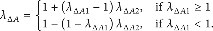
The final model obtained for λ_ΔA is as follows:

${\lambda }_{\Delta A}=\left\{\begin{array}{cc}1+({\lambda }_{\Delta A1}-1){\lambda }_{\Delta A2},\hfill & \text{if}\mathrm{\hspace{0.17em}\hspace{0.17em}}{\lambda }_{\Delta A1}\ge 1\hfill \\ 1-(1-{\lambda }_{\Delta A1}){\lambda }_{\Delta A2},\hfill & \text{if}\mathrm{\hspace{0.17em}\hspace{0.17em}}{\lambda }_{\Delta A1}<1.\hfill \end{array}\right.$

(10)

The three-dimensional surface plotted in Figure 4(d) illustrates the change in λ_ΔA with ΔA and R.

3. Driver Behavior When Entering and Exiting Curves

In related researches, two hypotheses concerning a driver's speed adjustment behavior when entering or exiting a curve were considered [7, 15, 16]. The first hypothesis pertains to the deceleration rate a _b and acceleration rate a _x . The most common assumption is that drivers adopt a fixed value of a _b (or a _x ) regardless of the curve radius. These may be two different values (for instance, a _b = 1.0 m/s² and a _x = 0.5 m/s²) or the same value (for instance, a _b = a _x = 0.8 m/s²). The second hypothesis pertains to where drivers adjust their speed. The most common assumption is that drivers complete their slowdown and speedup on the spiral segments before and after a circular curve, respectively. To verify these hypotheses, operating speeds were measured on twelve highways in the southwestern region of China. Figures 5(a) and 5(b) show the observation points and hidden location of the speed detector on typical road segments. At each location, operating speeds were measured for 20–30 cars. The average speed V _ai and 85th percentile speed V_85i at location i were used for various analysis purposes. The deceleration rate over a given distance can be calculated from two adjacent V _ai or V_85i values, as shown in Figures 5(c) and 5(d). The mean of a _bi is a _b for the curve considered, and a _x is calculated in the same manner as a _b .

Figure 5:

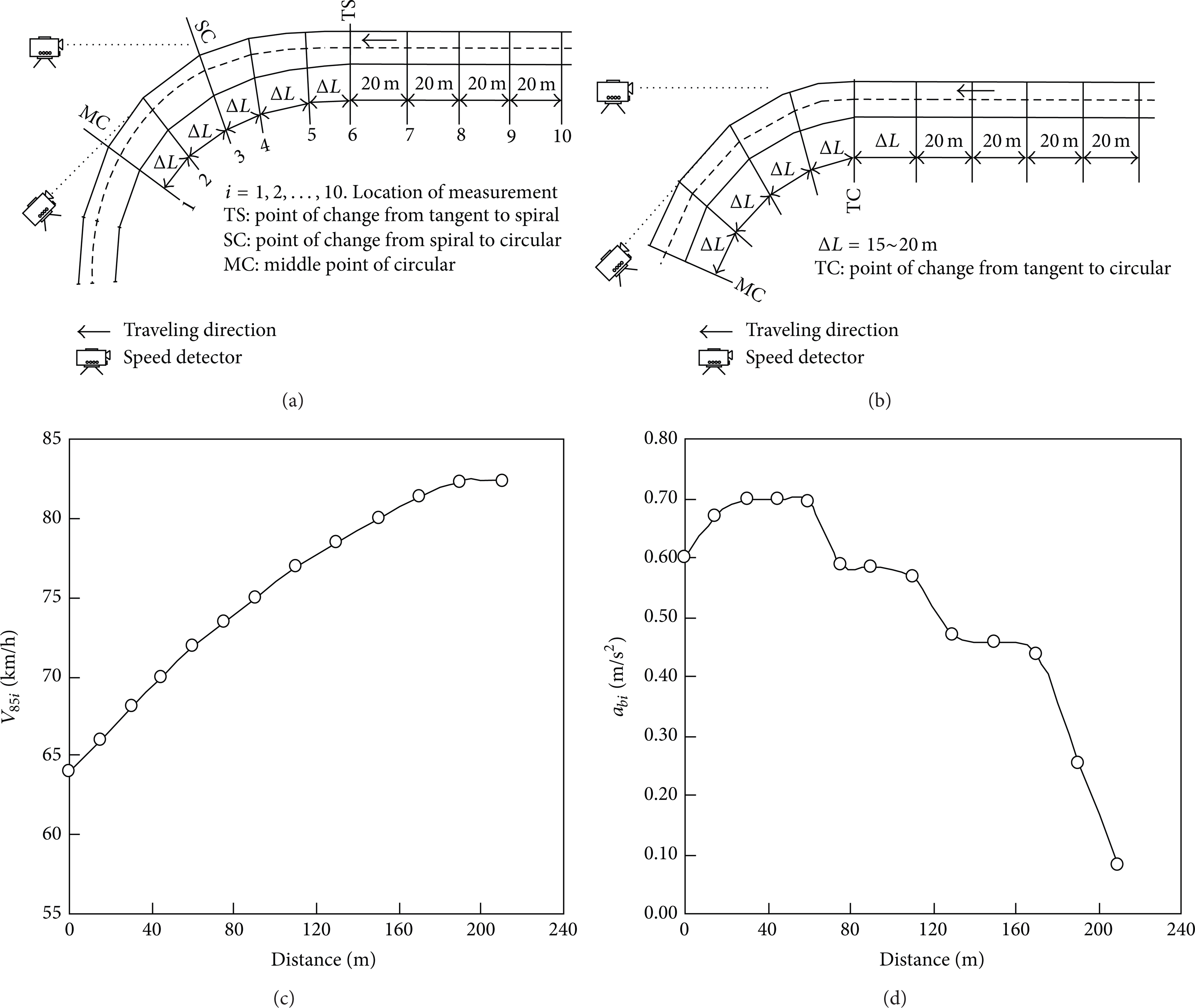
Speed measurement on the roadside to determine deceleration/acceleration rate of passenger cars: ((a), (b)) observed segments; (c) 85th percentile speed when entering curve; (d) a _bi versus distance.

Figures 6(a) and 6(b) show the results for a _b and a _x , respectively, for passenger cars on secondary rural roads, obtained as described above. According to the figures, the two hypotheses are inconsistent with observed driving behavior in two respects. First, both a _b and a _x vary with the curve radius. That is, the acceleration and deceleration rates are influenced by the curve geometry. Second, the deceleration rate is substantially greater than the acceleration rate for a given curve. Therefore, assuming that a _b and a _x are equal is inappropriate, and a model that can reflect the influence of curve geometry on a driver's speedup and slowdown behavior is needed.

Figure 6:

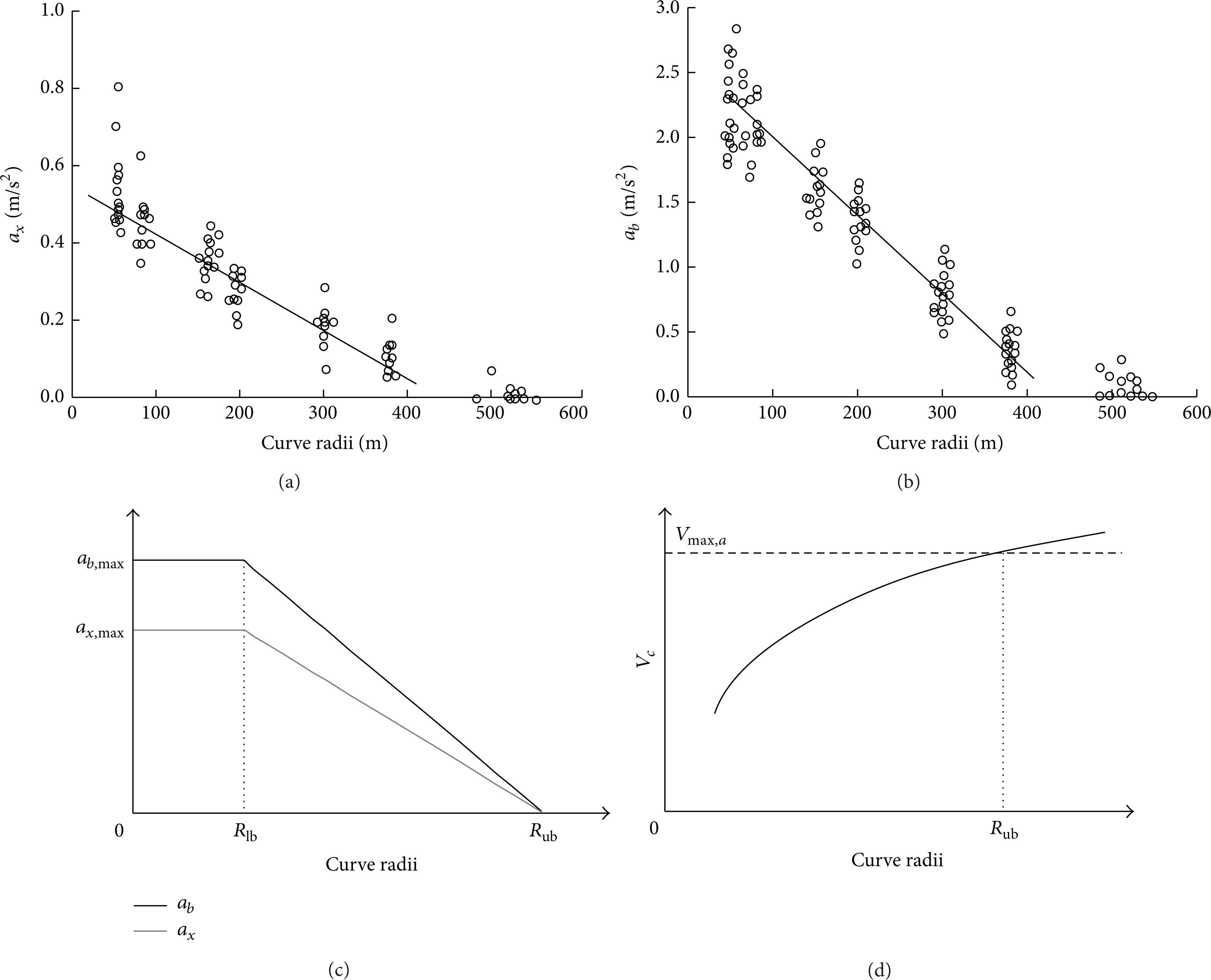
(a) a _b on secondary roads; (b) a _x on secondary roads; (c) a _b (and a _x ) versus curve radius; (d) relationship between V_{max ⁡} and R_ub.

The test data indicates that higher braking intensities are often adopted before drivers enter sharp curves. As the curve radius increases, the rate of deceleration decreases gradually and finally reaches zero point for a certain curve radius. The linear relations among a _b , a _x , and R can be described by the following equations:

$a_x=a_{x,\max }·f_r,\hspace{1em}\hspace{1em}{a}_b=a_{b,\max }·f_r,$

(11)

$f_r=\left\{\begin{array}{cc}1,\hfill & \text{if}\mathrm{\hspace{0.17em}\hspace{0.17em}}R\le R_{\text{lb}}\hfill \\ \frac{R_{\text{lb}}\times R_{\text{ub}}}{\left(R_{\text{ub}}-R_{\text{lb}}\right)\times R}-\frac{R_{\text{lb}}}{\left(R_{\text{ub}}-R_{\text{lb}}\right)},\hfill & \text{if}\mathrm{\hspace{0.17em}\hspace{0.17em}}{R}_{\text{lb}}<R<R_{\text{ub}}\hfill \\ 0,\hfill & \text{if}\mathrm{\hspace{0.17em}\hspace{0.17em}}R\ge R_{\text{ub}},\hfill \end{array}\right.$

(12)

where f _r reflects the effect of the curve radius on a _b and a _x and R_lb is the lower bound corresponding to the critical radius at which f _r no longer increases. The upper bound, R_ub, is the radius at which f _r decreases to zero. Figure 6(c) shows curves of a _b and a _x as functions of the curve radius, where a_{x, max ⁡} and a_{b, max ⁡} are the maximum acceleration and deceleration, respectively, adopted by a driver.

As with a_{y, tol}, the model parameters for a _b and a _x need to be calibrated with respect to the design speed of the road. The calibration ranges of the parameters, obtained from the experimental results, are given in Table 1. Note that the upper-bound radius R_ub needs to be calculated separately. Figure 6(d) shows that if a driver enters a curve with a radius greater than R_ub, there is no need to brake. In other words, the curve driving speed V _c calculated from a_{y, tol} and R is greater than the maximum speed V_{max ⁡, a} (defined in the following section) in this case. Therefore, R_ub can be obtained by solving (13). Because of the exponential function in this equation, an iterative method is useful in solving for R_ub:

$V_{\max ,a}^{\mathrm{2}}=V_c^2=a_{y,\text{tol}}\times R_{\text{ub}}=\left(a_{\text{lb}}+\frac{a_{\text{ub}}-a_{\text{lb}}}{e^{R_{\text{ub}}/C}}\right)R_{\text{ub}}.$

(13)

Table 1:

Calibrated values of model parameters a _b , a _x , and V_{max ⁡, a} for divided and two-lane highways.

Highway type	a x, max ⁡	a b, max ⁡	R min ⁡	R lb	R 2	b 0	b 1	b 2	γ	R 2
Expressway with 4–6 lanes	0.15–0.45	0.55–1.1	250–650	400–800	0.81	15	125–135	4-5	0.296	0.834
Two-lane highway	0.35–1.20	0.85–3.5	15–125	50–200	0.87	13.5	115–120	3.5–4.5	0.272	0.876

4. Maximum Travel Speed Controlled by Alignments

The maximum travel speed V_{max ⁡} often occurs on long tangents or curved segments with very large radii. Because of the development of new power trains in recent years, the major limitations to the maximum speeds of passenger cars on rural roadways are the pavement conditions and alignment design rather than the car's ability to accelerate. In general, for mountainous roads with complex shapes, the maximum speeds controlled by pavement conditions, V_{max ⁡, p}, are much higher than those controlled by alignments, V_{max ⁡, a}. Therefore, V_{max ⁡, a}, the lower of the two, is taken to be V_{max ⁡} for a given mountainous highway.

In this study, a model developed by Crisman et al. [17] was used to determine V_{max ⁡, a}. In this model, shown below, the roadway width W _R and curvature change rate CCR are the key controlling factors of the maximum possible speed on a roadway:

$V_{\max }=V_{\max ,a}=b_{\mathrm{0}}+b_{\mathrm{1}}\times {\text{CCR}}^{-\gamma }+b_{\mathrm{2}}\times W_R,$

(14)

where CCR = 1000 × ∑α _i /L _R , W _R = N _L × W _L + W_EL + 2W _S , α _i is the curve deflection angle, L _R is the road length, W _L is the lane width, W _S is the shoulder width, and W_EL is the emergency lane width.

Data on the driving speeds of passenger cars on long straight sections of highways with flat or slight grades in southwestern China were used to recalibrate the model parameters b₀, b₁, b₂, and γ with respect to the design speed, as shown in Table 1.

5. Process for Computing Desired Speed

Using the models presented previously, a driver's desired speed V_de on an arbitrary roadway can be determined from the given geometric alignment and design speed of the roadway. The main steps in the calculation process are as follows.

(1) Calculate the maximum speed V_{max ⁡, a} as the controlling value for the desired speed, as shown in Figure 7(a).

Figure 7:

(a) V_de on tangents and circular curves; (b) V_de reaches maximum value on tangents; (c) deceleration begins before V_{max ⁡} is reached.

(2) Select model parameters from Table 1 according to the design speed of the roadway, calculate a_{y, tol} using (1), and then use

$V_c=\mathrm{3.6}\sqrt{R\times a_{y,\text{tol}}}$

(15)

to calculate the preliminary speed V _c on the curve.

(3) Use (6) to calculate the lane width influence coefficient λ _w , use (10) to calculate the deflection angle influence coefficient λ_ΔA if its effect is to be considered, and obtain V _c using

$V_c=\mathrm{3.6}\sqrt{R\times a_{y,\text{tol}}\times {\lambda }_w\times {\lambda }_{\Delta A}}.$

(16)

(4) Take the lower of V _c and V_{max ⁡} as the desired speed on the curve, as shown in Figure 7(a).

(5) Use (11) to calculate the curve entering deceleration rate a _b and the curve leaving acceleration rate a _x , and calculate the slowdown distance L _b and speedup distance L _a using

$L_b=\frac{(V_{\max }^{\mathrm{2}}-V_{\text{ci}}^{\mathrm{2}})}{a_b},\hspace{1em}\hspace{1em}{L}_a=\frac{(V_{\max }^{\mathrm{2}}-V_{\text{ci}}^{\mathrm{2}})}{a_x}.$

(17)

(6) Determine the control points on the roadway for changing speed. When there is a sufficiently long tangent before and after a curve, the starting point of braking and the ending point of throttling can be determined directly using L _b and L _x , as shown in Figure 7(b). However, for winding roads, the tangent between neighboring curves is often very short, and in some cases, there may not even be a tangent between curves. Therefore, the speed adjustment for the next curve has to be performed while the vehicle is in the current curve. Figure 7(c) shows how the tangent length influences the desired speed.

6. Simulation Experiments with Various Types of Drivers

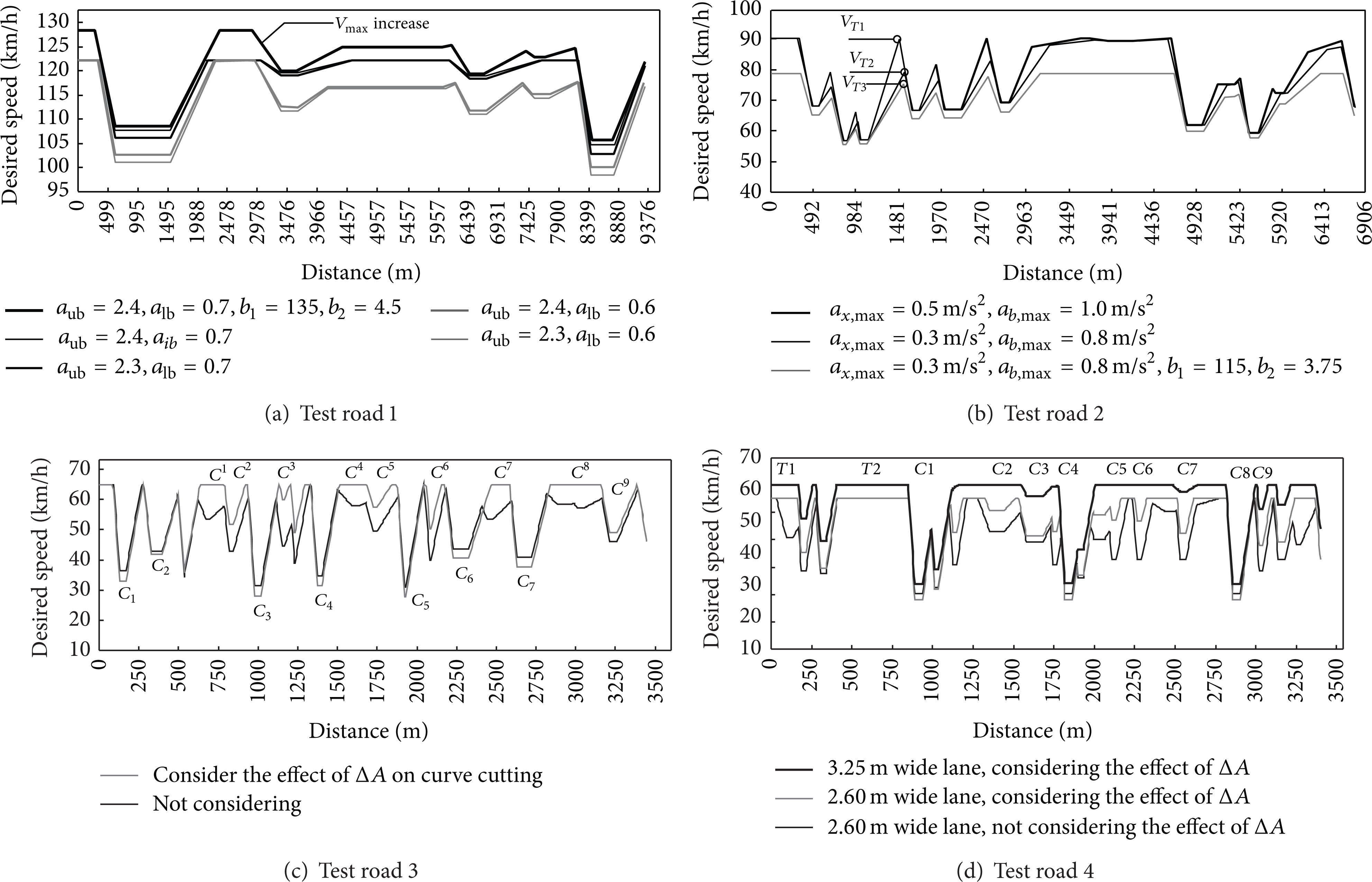
Variations in driving speed occur on all types of roadway segments, whether tangents or curves. The factors that contribute to variation in speed can be classified in two categories. One category consists of factors related to the driver's characteristics. In terms of speed choice preference, drivers can be divided into three types: impulsive, intermediate, and conservative. The other category consists of factors related to the dynamic performance of the vehicle. For example, the Suzuki minibus with poor dynamic performance has a below-average speed, and its acceleration and deceleration rates are often lower than other passenger cars in most situations. By setting combinations of a_{y, tol}, V_{max ⁡}, λ_ΔA, λ _w , a _x , and a _b , the characteristics of the three types of drivers and the performance of different passenger cars can be considered. Figure 8 shows a set of four test roadways used in this study to demonstrate how model parameter combinations influence the desired speeds for the three driver types.

Figure 8:

The horizontal alignment of test road. (a) Test road 1; (b) test road 2; (c) test road 3; (d) test road 4.

Test road 1 was an expressway segment with a design speed of 100 km/h, three lanes in each direction, curve radii of 800–3000 m, and an average curve radius of 1450 m. Test road 2 was a secondary two-lane road with a design speed of 60 km/h, a total roadway width of 8.5 m, curve radii of 125–1200 m, and an average curve radius of 434.45 m. Test road 3 was a tertiary two-lane rural road with a design speed of 30 km/h, a total roadway width of 7 m, curve radii of 32–450 m, and an average radius of 118.33 m. Test road 4 was a fourth-class road segment with a design speed of 20 km/h, a total roadway width of 5.2 m, curve radii of 15–300 m, and an average curve radius of 70.31 m.

6.1. Effects of Model Parameters $a_{y,\text{tol}}$ and V_{max ⁡} on Desired Speed

Because a higher V_{max ⁡} is used when the driver's tolerable lateral acceleration a_{y, tol} increases, the model parameters a_{y, tol} and V_{max ⁡} are correlated. Figure 9(a) shows that when a_ub and a_lb (parameters used to determine a_{y, tol}) increase, V _c on the curve increases. V _c is much more sensitive to an increase in a_lb than to an increase in a_ub. Therefore, the speed control of impulsive drivers can be simulated by increasing a_ub and a_lb. In contrast, relatively low parameter values should be used for conservative drivers. If only a_ub and a_lb increase, the driver's speed control cannot be reflected in speed profiles, as the speed on curve V _c exceeds V_{max ⁡}. To reflect the change in speed, V_{max ⁡} should increase as well. Therefore, the ideal design strategy for the parameter combination of impulsive drivers would be that a_ub and a_lb increase with b₁ and b₂ (see the top profile in Figure 9(a)).

Figure 9:

Desired speed profiles on test roads 1–4.

6.2. Effects of Model Parameters a _x and a _b on Desired Speed

The driver type is a factor that influences the deceleration of an automobile in a curve. An impulsive driver often slows down with powerful braking when approaching a sharp curve at the end of a tangent and is eager to speed up at an unusually high acceleration rate when leaving the curve. In Figure 9(b), when the parameters used to determine a_{y, tol} and V_{max ⁡} are fixed and only a_{x, max ⁡} and a_{b, max ⁡} are decreased, the desired driving speed on the tangent between the adjacent two curves decreases (as shown in Figure 9(b), V_T1 > V_T2 > V_T3). In fact, relatively low a_{x, max ⁡} and a_{b, max ⁡} are commonly used by conservative drivers or those driving vehicles with poor dynamic performance. To ensure safety, these drivers reserve a relatively higher margin of lateral acceleration a_{y, mar}, which results in lower a_{y, tol} and V_{max ⁡} while the critical lateral acceleration remains constant. Therefore, a_{y, tol} and V_{max ⁡} should be adjusted simultaneously when the parameters a_{x, max ⁡} and a_{b, max ⁡} are decreased. Consequently, the rational desired speed profile should be the lowest one in the figure.

6.3. Effect of Deflection Angle on Driving Speed

A smaller deflection angle ΔA means that the curve can be cut more easily. Therefore, ΔA has a large influence on the driving speed, especially for impulsive drivers. Figure 9(c) shows that the effect of ΔA can lead to two types of changes in the desired speed. First, the desired speed is higher on curves with small ΔA, such as the curves marked C¹–C⁹ in the figure. On curves C¹, C⁴, C⁷, and C⁸, the desired speed reaches the maximum traveling speed V_{max ⁡}, which means that there is no need for braking when drivers cut the curve. Second, a large ΔA can decrease the desired speed, as in the cases of curves C₁–C₇, because a large ΔA can not only restrict the occurrence of curve cutting but also obstruct the visibility of roadway features ahead.

6.4. Effect of Lane Width on Driving Speed

Figure 9(d) shows the changes in the desired speed on test road 4 before and after the driving lane was widened from 2.6 m to 3.25 m, as well as the changes with and without consideration of the effect of ΔA. Widening a lane can increase the desired speed on tangents or curves. However, the amount by which a vehicle's speed changes is different for each of three different types of curves. For curves with large ΔA, such as C1, C4, and C8, the desired speed changes the least—slightly less than that on a tangent. Moreover, the speed can be decreased on such curves because of the large ΔA. For curves of the second type, such as curves C3, C7, and C9, the desired speed significantly increases after the lane is widened because more driving space is provided for drivers to use. The curvature of the vehicle's trajectory decreases, and the driver can thus select a higher speed. For curves of the last type, such as curves C2, C5, and C6, the desired speed exceeds V_{max ⁡}. The driver can therefore maintain a constant speed of V_{max ⁡} before, in, and after the curve. Thus, he or she can negotiate such curves without braking, which is similar to driving on long tangents.

7. Automated Driving in a Virtual Environment

To validate the model for driver speed control behavior, a computerized road-driver-vehicle simulation system was developed. The software package ADAMS was used to create a dynamic model of a full passenger car. A roadway creation module was developed using the VB 2010 Enterprise edition, in which the three-dimensional shapes of road surfaces can be obtained from the design elements of the horizontal and vertical alignments and cross section. After the friction coefficients of the road surface are set, the interaction between the pavement surface and tires can be simulated. A driver module (including speed and steering control models) was also developed using VB 2010, and a “preview” strategy was adopted in the steering and speed control algorithms. Road 3 in Figure 8 was selected as the test road. Using the models developed in this study, the desired speed V_de along the road was determined. The acceleration and deceleration rates at each position on the road, as well as the change rates of the throttle and/or brake, were computed using the speed control module based on the profile.

In the driving simulation process, operating instructions for speed control were transmitted to actuators of the car model if the actual driving speed of the car deviated from V_de. Figure 10(a) illustrates the car model driving on a three-dimensional roadway that includes curvature, a pavement width, a bank, a slope, and a widened inner lane on sharp curves. Figure 10(b) shows the desired speed, actual driving speed, and critical safety speed for roadway departure prevention, as developed by Sentouh et al. [10]. The profiles shown in Figures 10(c) and 10(d) are the longitudinal and lateral acceleration, respectively, along the traveled distance. The results indicate that the desired speed determined using the models developed in this study can serve as the ideal target speed for a passenger car and satisfy the dynamic performance requirements for an automated vehicle on roads with complicated shapes. Furthermore, traffic safety can be ensured when the vehicle follows the desired speed, as the profile of V_de is always below the critical speed.

Figure 10:

Simulation results for automated car on test road 3: (a) illustration of car on road; (b) desired speed, driving speed, and critical safety speed; (c) acceleration and deceleration rates; (d) lateral acceleration.

8. Conclusions

Using data from actual driving experiments and spot speed observed on roadside, the relationship between roadway geometry features and drivers' speed choice behavior was analyzed. The goal of this analysis was to understand how roadway geometry affects a driver's speed control. Models were established for a driver's speed choice on curves, entering and exiting curves, and on tangents. The desired speed on any given road segment can be obtained using these models. The type of driver and the dynamic performance of the vehicle can also be considered by combining the parameters of the various models. The effectiveness and stability of the models were demonstrated using a computer-based driving simulation on a narrow winding road. The results of this research can be applied to the development of algorithms for intelligent driving systems for passenger car travel on roads with complicated shapes.

Conflict of Interests

The authors declare that there is no conflict of interests regarding the publication of this paper.