Investigation of Transient Flow in a Centrifugal Charging Pump during Charging Operating Process

Abstract

Centrifugal charging pumps are important components of nuclear power plants and must be operated under multioperating conditions for the requirements of the system. In order to investigate the internal flow mechanism of the centrifugal charging pump during the transient transition process of charging operating from Q = 34 m³/h to Q = 110 m³/h, numerical simulation and experiment are implemented in this study. The relationship between flow rate and time is obtained from the experiment and worked as the boundary condition to accurately accomplish the numerical simulation during the transient process. External and internal characteristics under the variable operating conditions are analyzed through the transient simulation. The results show that the liquid viscosity, large scale vortexes exist in the flow passages in the beginning of the variable operating conditions, which indicates flow separation and the sudden changes in direction of velocity. As the flow rate increases gradually, the flow angles of the fluid in inlet accelerate correspondingly and the flow along the blade is more uniform, which leads to a decrease and movements of the vortexes. The contents of the current work can provide references for the design optimization and fluid control of the pump used in the transient process of variable operating conditions.

1. Introduction

Centrifugal charging pumps used in pressurized water reactors (PWR) are components which are critical to nuclear plant operations. They are parts of the chemical and volume control system (CVCS) and are designed to provide normal charging service to the reactor coolant system (RCS) [1], which makes them extremely important in nuclear power plants. In nuclear plant systems, the pumps must be operated under multioperating conditions accurately and the valve adjusting time between two adjacent operating conditions is required to be less than 10 seconds. The vortex, backflow, flow separation, and pressure fluctuation are generated unavoidably during the valve opening process from one flow rate to another in such a short time. These transient characteristics, which come from charging pumps, may lead to facility or power system destruction. Thus it attaches great importance to the investigation of the transient flow during the process of variable operating conditions of the centrifugal charging pump.

Transient process of many kinds of pumps existed in various occasions, such as starting period, stopping period, and the flow-rate variation period. The flow characteristics during the transient process are different from steady process. There have been lots of researches on transient characteristics during starting and stopping process in the past few decades. Tsukamoto et al. [2, 3] analyzed the transient characteristic during stopping period and startup period of a centrifugal pump by using both numerical and experimental methods. It was concluded that the curves of dimensionless flow and dimensionless head recovered to a steady level after they dropped sharply below the steady results. Zhang [4] used moment conservation law to build up a series of equations of the pump system. The head and flow rate change rules were obtained from the equations. Moreover, the transient characteristics were obtained by the steady-state head curve. Lefebvre and Barker [5] carried out experiments on hydrodynamic performance of a centrifugal pump during transient operation. It showed that there was deviation in the results between transient process and quasi-steady assumptions. Thanapandi and Prasad [6] originally analyzed the dynamic performances during starting and stopped periods by a numerical model using the method of dynamic characteristics. The model can be applied for analyses of purely unsteady cases where the pump dynamic characteristics show considerable departure from their steady-state characteristics. Li et al. [7, 8] used computational fluid dynamics to study the three-dimensional unsteady incompressible viscous flows in a centrifugal pump during rapid starting period (0.12 s). The rotational speed variation of the field around the impeller was realized by a dynamic slip region method, which combined the dynamic mesh method with nonconformal grid boundaries. They also used PIV technique to capture transient flow evolutions in the pump and drew a conclusion that the transient vortex evolution between blades was more important than reversed flow at the blade inlet to the transient head coefficient. Ma et al. [9] used a hydraulic-force coupling method to simulate the transient process of power failure condition. They pointed out that the differences between transient and quasi-steady results were caused by the inertia effect of fluid contained in the pump and the pipeline. Wu et al. [10–12] presented two numerical methods based on finite volume method (FVM) to solve the transient rotating flow induced by a speed-changing impeller. They have investigated the transient hydrodynamic performances of centrifugal pumps during transient operation like different starting acceleration rates and the discharge value rapid opening process.

However, the investigations mentioned above were focused on the transient processes of startup period and stopping period. There is almost no research concerning the transient characteristics during the process of variable operating conditions. So it is extra urgent to investigate the transient characteristics during this process.

Nowadays, with the development of CFD technology, numerical simulation has been greatly developed and widely used in the transient flow calculation. In this paper, both experimental and numerical methods are used to investigate the transient characteristics during the process from charging condition (Q = 34 m³/h) to the highest efficiency condition (Q = 110 m³/h). The simulation is validated by comparing the experimental results. Afterwards the internal transient flow characteristics are obtained through numerical simulation and compared with the steady-state flow performances. The differences between transient flow and steady-state flow are obvious and the results can be used as reference for future studies and applications.

2. Numerical Methods

2.1. Calculation Model

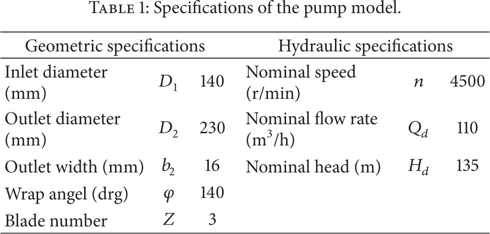
In this study, the research object is a 12-stage centrifugal pump. The first stage of the charging pump is selected to investigate the transient characteristics during the process of variable operating conditions. The 3D geometry structures, including the inlet section, impeller, and double channels volute, are shown in Figure 1. The pump is designed to rotate at n = 4500 r/m and the specifications of the model pump are given in Table 1.

Table 1:

Specifications of the pump model.

Geometric specifications			Hydraulic specifications
Inlet diameter (mm)	D 1	140	Nominal speed (r/min)	n	4500
Outlet diameter (mm)	D 2	230	Nominal flow rate (m3/h)	Q d	110
Outlet width (mm)	b 2	16	Nominal head (m)	H d	135
Wrap angel (drg)	φ	140
Blade number	Z	3

Figure 1:

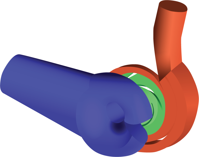
3D model.

2.2. Mesh Generation

After being modeled in Pro/E, the calculation domains are imported to ICEM CFD 12.1 for mesh generation. The mesh grids are not only expression forms of geometry but also the carrier of simulation and analysis [13]. Tetrahedral unstructured grids are selected in the inlet and the double channels because of their confused structures. The impeller is the most important component, so the flow fields around the blades are meshed hexahedral structured grids.

2.3. Grids Independence

With the increase of grids number, the error caused by the grid will be reduced gradually until it disappears. Grids independence study is conducted by solving the flow for five different numbers varying from 1.22 million to 2.54 million. The heads are compared under 5 different cases of grids numbers, as shown in Figure 2. It can be seen that the head rose up with the grids number increase, but it keeps constant nearly after the number exceeded 2.35 million. Considering the configuration of the computer and computing time, the number of grids cannot be too large. The total grid number is 2.35 million which can not only guarantee the simulating precision but also shorten the design period.

Figure 2:

Head with different grids number.

2.4. Turbulence Model

It is necessary to select the turbulence model most suitable for the fluid domains to be calculated and to carefully validate it because the turbulence model describes the Reynolds stresses distributions in the flow domains. What is more is that the flow fields at off-design conditions are highly turbulent and unsteady. Due to the complex separation and recirculation during the transient flow process, a reliable turbulence model selection is extremely important to simulate the performances more accurately. Because the turbulent flow in charging pumps developed absolutely under high rotating speed, the standard k-εis selected to solve the Reynolds-Averaged Navier-Stokes equation in this paper.

2.5. Boundary Conditions

The flow rate exhibits nonlinear variation among the different operating conditions. The function of the flow rate based on experimental data during the transient process is set in the CEL of CFX, which is defined as the outlet boundary, while the total pressure is defined as the inlet boundary.

The whole hydraulic passages in the first stage of charging pump are taken as the computational flow domains. All physical surfaces of the pump are set as no-slip wall. Considering the limitation of the manufacture techniques, the surface roughness is set as 10 micron for all the flow domains to close the gap between simulating results and test results. The flow in the impeller is defined as rotating zone and the flow in the inlet and double channels volute is calculated in the stationary reference frame. The connection between the impeller and the stationary components is linked by interfaces. Because the relative position between the impeller and the volute changes for each time step with this kind of interface, the frame change for the interface between the rotor and stator is set as transient rotor stator. The GGI is set as the method of mesh connection.

2.6. Monitoring Points

Some monitoring points are set in flow passage of the charging pump in order to analyze the flow characteristics more clearly. There are five monitoring points located on the impeller from inlet to outlet, while also five monitoring points are set in the flow passage of the double channels volute. The monitoring points in the impeller and the volute are shown in Figure 3.

Figure 3:

Distributions of monitoring points.

Before the transient simulation, the unsteady case was presimulated to get the initial condition of transient process.

3. Experiment

3.1. Test Rig

Hydraulic tests are carried out by closed-type test rig with China national 1-grade precision at Jiangsu University, as shown in Figure 4. The charging pump, pipes, water tank, valves, and turbine flow meter constitute the closed loop recirculation system. All flow passages, water tank, and the pump are filled with 25°C water with density of ρ = 1000 m³/h and dynamic viscosity of μ = 0.001 pa·s. Instantaneous flow rates are measured by the turbine flow meter installed at the outlet section of the charging pump body. Instantaneous static pressures are obtained by the pressure transducers installed at the inlet and outlet pipes. All the signals are transmitted to the data acquisition card and the LabVIEW virtual instrument platform.

Figure 4:

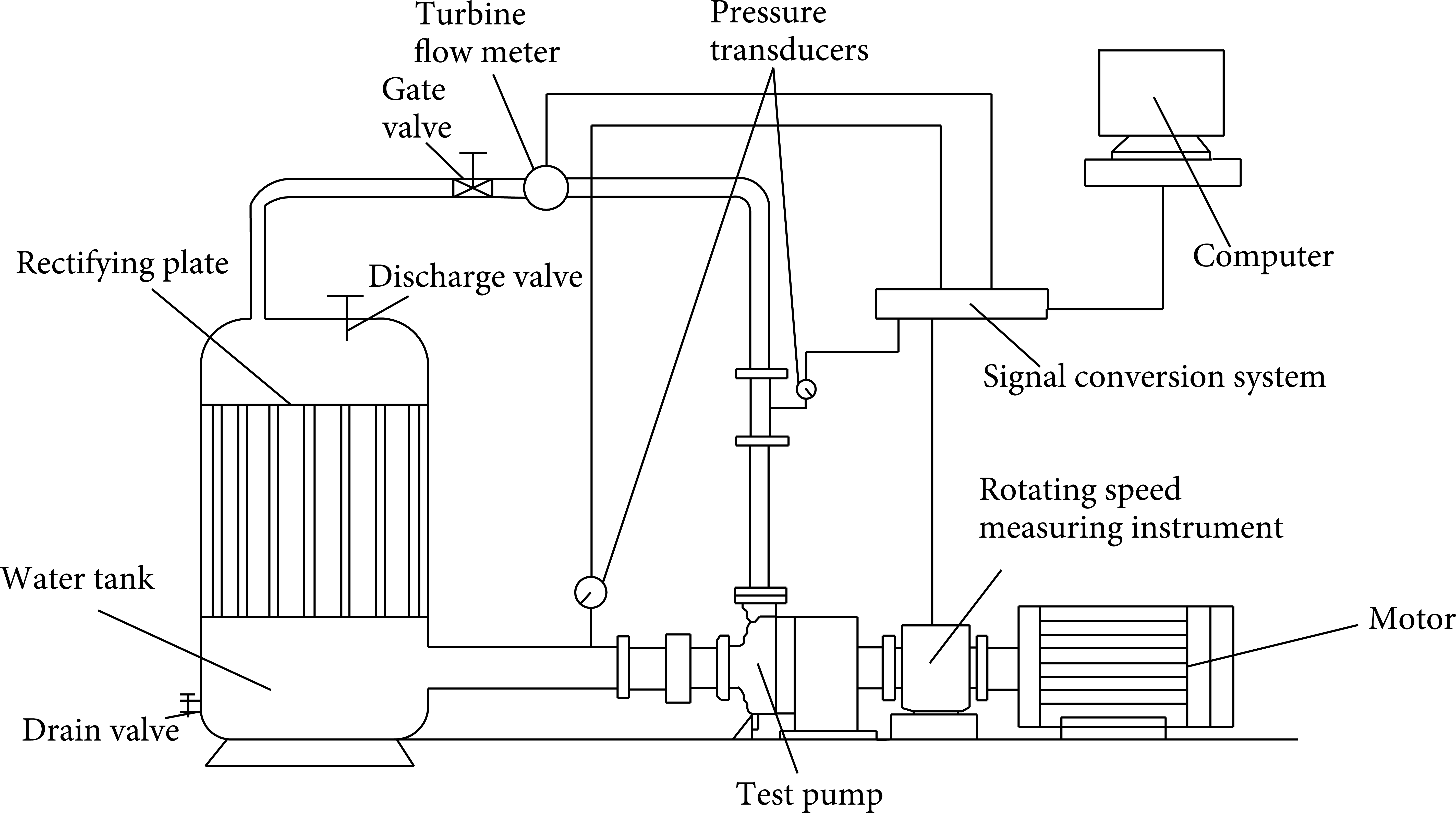
Test rig.

The charging pump flow passage is formed by the inlet, the first stage impeller, double channels volute, and pump body. The axis cross-section of the charging pump with first stage is shown in Figure 5 and the operating points of the charging pump are shown in Table 2. The transformation of the flow rate from one operating point to another operating point is achieved by adjusting the gate valve within 10 seconds.

Table 2:

Operating points of the charging process.

Charging operation condition
Nominal condition	Highest efficiency
34 m3/h	110 m3/h

Figure 5:

Axis cross-section of the charging pump.

3.2. Test Results

The impeller is driven by the motor with a rotational speed of 2950 r/min and a similar conversion theorem is used to obtain the corresponding flow rates in each operating point. Head comparison between simulated and experimental results is shown in Figure 6. The trend of the experimental result is consistent with the simulated result and most of the experimental heads are no more than 1 m below the simulated heads ranging from 34 m³/h to 110 m³/h. It is within the acceptable difference between the experimental and simulated results because of the mechanical losses.

Figure 6:

Head comparison between simulation and experiment.

It took 2.5 seconds to achieve the transformation of the flow rate from 34 m³/h to 110 m³/h in the experiment. The experimental result of the Q-t curve is shown in Figure 7 and the function of Q-t curve is set in CEL of CFX as the boundary condition of the outlet. A key feature of CEL is that it is used dynamically by the CFX-Solver, and the transient flow characteristics will be computed based on the variable flow rates. Figure 8 shows detailed settings of flow rate in CEL.

Figure 7:

The flow rate during the transient process.

Figure 8:

Flow rate settings in CEL expression.

Internal flow of the pump is changed continuously with the flow rate. Every 30° of the impeller is recorded in a rotating circle during the transient process and total time is 2.5 s, so the time step is 0.0011 s and the flow field needs to be iterated for 2250 steps. The previously calculated results of flow field are used as the initial flow field for transient flow simulation.

4. Results and Discussion

4.1. Comparison of External Characteristics between Steady and Transient Process

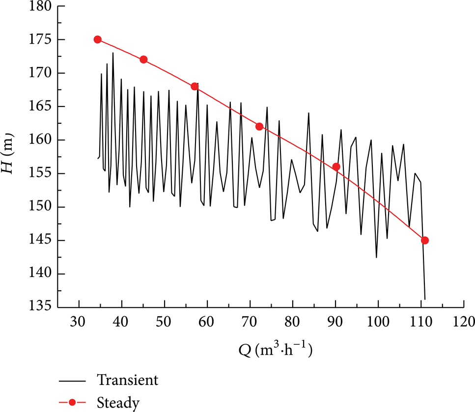
Simulated heads of steady-state and transient process are shown in Figure 9. There is great deviation of the heads between the instantaneous state and the steady state, as can be seen from the graph. The average head of transient process lies under the head in the steady state before Q = 90 m³/h and then it exceeds the steady-state result from Q = 90 m³/h to Q = 110 m³/h. With the flow rate increasing, the transient head curve approaches the steady-state curve gradually. This is because the flow rate increases to the highest efficiency operating point and the flow separation lessens in the impeller, causing the transient curve to move closer to the steady-state curve.

Figure 9:

Head comparison between steady and transient simulation.

4.2. Pressure during the Transient Process

4.2.1. Pressure Fluctuation

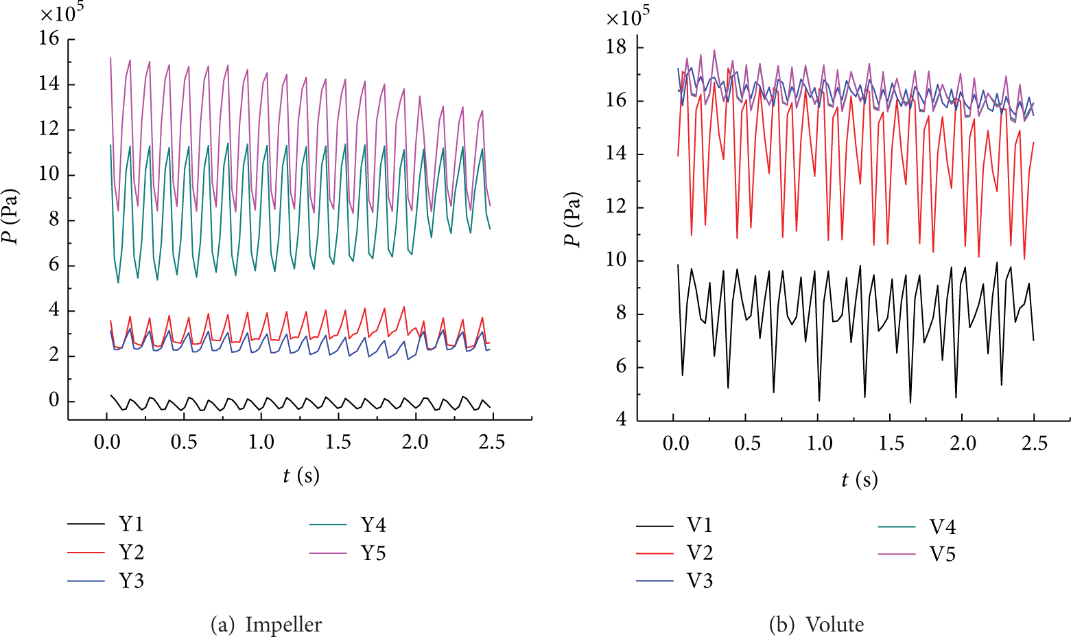
When the flow rate increases from the charging condition (Q = 34 m³/h) to the highest efficiency condition (Q = 110 m³/h), the transient pressure curves of monitoring points in the impeller and the double channels volute are shown in Figure 10.

Figure 10:

Transient pressure from 34 m³/h to 110 m³/h.

It could be seen that the pressure fluctuations of the monitoring points in the impeller are not uniform from Figure 10. The pressure of each monitoring point in the impeller increases gradually to the maximum and then decreases to the minimum in a rotational circle and looks like a sinusoidal curve. The rotor-stator interaction between the rotation of the impeller and the volute causes dozens of times of pressure fluctuation. Pressure fluctuations of the monitoring points near the interface between the impeller and the volute are bigger than others. As the monitoring points Y4 and Y5 are more vulnerable to the interference between the impeller and the volute, the pressure fluctuation amplitudes of Y4 and Y5 are 3~5 times larger than those of other monitoring points in the impeller. The flow is untidy in the flow passage and it causes large vortex in the small flow rate at the beginning of the variable operating conditions. As the flow rate increases, flow separation on the blade surface decreases, which leads to a movement of the vortexes, so the fluctuant amplitudes of the transient pressure are large and then reduce gradually during the transient process.

As for the rotation of the impeller, it could be seen clearly that the pressure fluctuation of the monitoring points V1 and V2 in inside channel is more serious than that of V3, V4 and V5 in the outside channel of the double channels volute. The pressure fluctuation amplitudes of V1 and V2 are 5~8 times larger than those of V3, V4 and V5. So the pressure fluctuation amplitude in outlet of the volute could be reduced by the double channels volute chamber. The pressure fluctuation amplitudes of all monitoring points in the volute keep constant nearly with the flow rate increasing. This indicates that the pressure of the volute is influenced hardly by the variable operating conditions.

4.2.2. Pressure Distributions in the Impeller

The pressure distributions on the cross-section of the impeller at different times during the transient process are, respectively, shown in Figure 11. As can be seen from the graphs, the pressure appears to suddenly change at the beginning of the transient process and the distributions become more and more uniform with the flow rate increasing to the highest efficiency. Pressure gradually decreases from working surface to back surface, while regularly increasing from inlet to outlet of the impeller. When the impeller rotates near the two tongues of the volute, the pressure is higher than that in other parts of the impeller because the flow near the tongues is unsteady. They are consistent with the results discussed in the above chapter.

Figure 11:

Pressure distributions in the impeller.

4.2.3. Pressure Distributions in the Volute

The pressure distributions in the cross-section of the volute at different times during the transient process are, respectively, shown in Figure 12. It can be seen clearly that the pressure distributions are untidy in the small flow rate and there is an obvious super high pressure zone near the tongue under the flow rate Q = 34 m³/h. The two volute tongues make flow field present unsymmetrical structure, while, except for the two-volute-tongue region, distribution of the pressure in the volute is uniform. Being the same with the impeller, the pressure distributions in the volute get more regular with the flow rate increasing, which shows better performance at the end of the transient process.

Figure 12:

Pressure distributions in the volute.

4.3. Streamline during the Transient Process

4.3.1. Streamline Distributions in the Impeller

The streamline distributions in the cross-section of the impeller at different times are given in Figure 13. It can be seen from the graph that large scale vortexes exist in the impeller near the volute tongue at the small flow rate, which indicates the sudden changes in direction of velocity, and so it lowers efficiencies of the pump inevitably. This is because fluid flows out from the wall surface on account of small fluid momentum in the boundary layer. The areas where fluid velocity closes to zero generate vortexes. As the flow rate increases gradually, more compact vortexes are occurred in the flow passage of the impeller, while vortexes in the case are smaller. The main reason is that flow separation occurs on the blade surface due to liquid viscosity at off-design operating conditions and thus vortexes are occurred. There is almost no vortex in the impeller after t = 2 s and the streamlines are getting much more regular, and the flow pattern reaches the best at the flow rate Q = 110 m³/h. This is because flow separation on the blade surface decreases with the flow rate increasing.

Figure 13:

Streamline distributions in the impeller.

4.3.2. Streamline Distributions in the Volute

The streamline distributions in the cross-section of the volute at different times are given in Figure 14. The vortexes block the volute tongues at t = 0 s (namely, Q = 34 m³/h), which causes the increase of hydraulic loss and the decline of explicit performances inevitably. With the flow rate increasing, the vortexes strength quickly weakens and becomes less evident. When t reaches 2.5 s (namely, Q = 110 m³/h), the streamlines in the volute become smooth and tidy, which shows that the flow pattern is the best at the end of the transient process.

Figure 14:

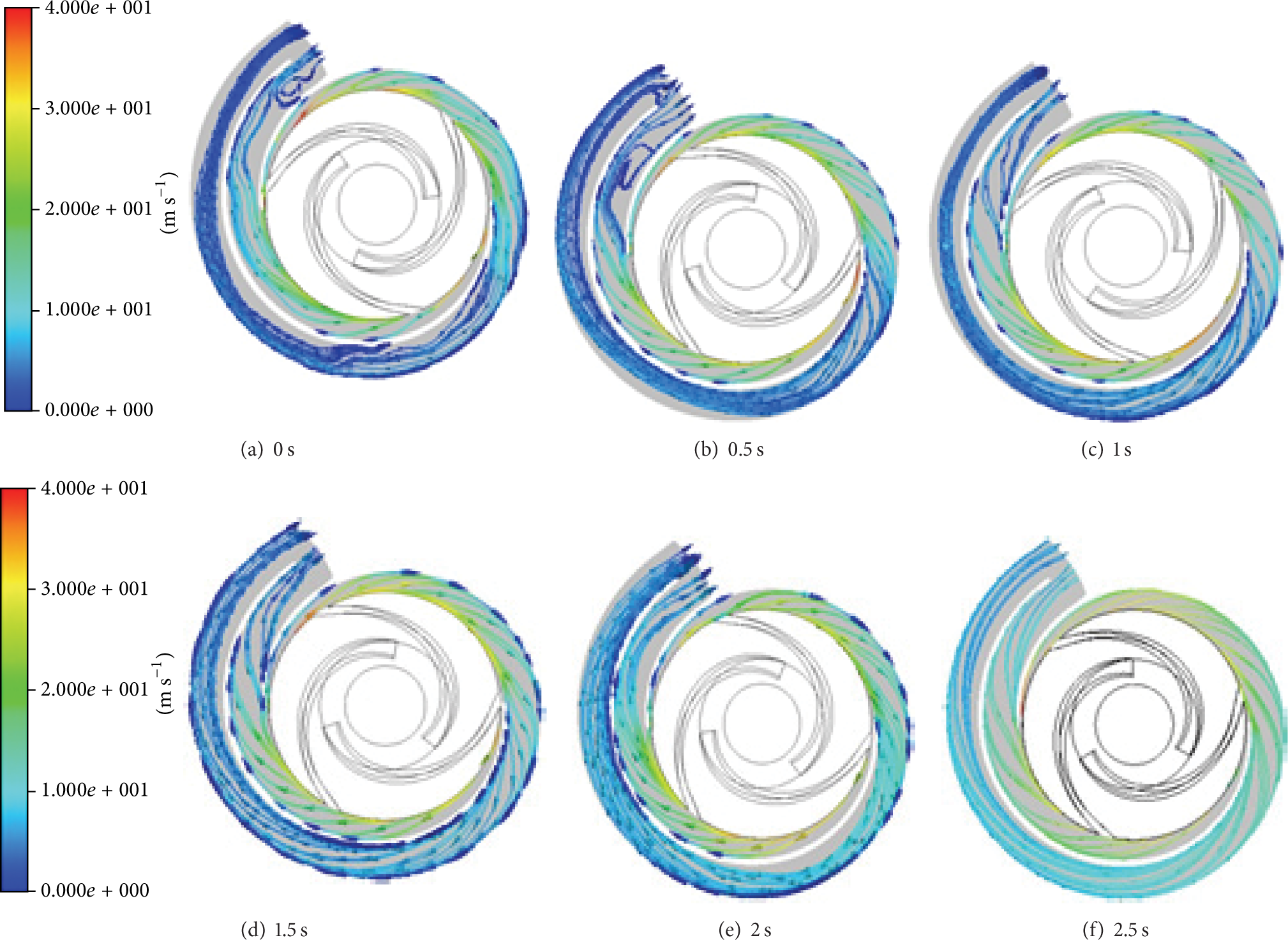
Streamline distributions in the volute.

5. Conclusions

The transient process during the variable operating conditions from the charging operating condition (Q = 34 m³/h) to the highest efficiency operating condition (Q = 110 m³/h) is investigated through numerical and experimental methods in this paper. According to the simulating and experimental results, both external hydrodynamic characteristics and internal flow pattern during the transient process are analyzed in the following aspects.

1. Comparisons with the experimental results verify the validity in simulating the instantaneous flow in the first stage of the charging pump under the transient process. The transient flow pattern is well indicated through numerical simulation.

2. In the beginning of the transient process, fluid flows out from the wall surface on account of small fluid momentum in the boundary layer. The areas where fluid velocity closes to zero generate vortexes. As the flow rate increases, the flow angles of the fluid in inlet accelerate correspondingly and the tangent of the angle is consistent with the direction of the rotation, which leads to a decrease and movements of the vortexes. So the flow in the pump is more and more uniform during the transient process. Besides the effect of the flow acceleration, a transits effect of the vortexes revolution is also a main factor which influences the flow pattern of the charging pump.

3. Rotor-stator interaction makes the distribution of pressure in the flow passage vary obviously. The two tongues in the volute make flow field present unsymmetrical structure, while, except for the two-volute-tongue region, distribution of the pressure in the volute is uniform.

4. Due to the liquid viscosity, large scale vortexes exist in the flow passages at the small flow rate, which indicates flow separation and the sudden changes in direction of velocity. As the flow rate increases gradually, more compact vortexes are occurred but vortexes in this case are smaller. The amplitude of the transient pressure fluctuation tends to decrease gradually and the flow pattern becomes the best at the end of the transient process.

In order to explain the mechanisms of the instantaneous flow evolutions more clearly during the transient process, experimental flow test techniques, such as high-speed photography and PIV, will be expected in further study.

Conflict of Interests

The authors declare that there is no conflict of interests regarding the publication of this paper.