Surface Roughness and Residual Stresses of High Speed Turning 300 M Ultrahigh Strength Steel

Abstract

Firstly, a single factor test of the surface roughness about tuning 300 M steel is done. According to the test results, it is direct to find the sequence of various factors affecting the surface roughness. Secondly, the orthogonal cutting experiment is carried out from which the primary and secondary influence factors affecting surface roughness are obtained: feed rate and corner radius are the main factors affecting surface roughness. The more the feed rate, the greater the surface roughness. In a certain cutting speed rang, the surface roughness is smaller. The influence of depth of cut to the surface roughness is small. Thirdly, according to the results of the orthogonal experiment, the prediction model of surface roughness is established by using regressing analysis method. Using MatLab software, the prediction mode is optimized and the significance test of the optimized model is done. It showed that the prediction model matched the experiment results. Finally, the surface residual stress test of turning 300 M steel is done and the residual stress of the surface and along the depth direction is measured.

1. Introduction

300 M steel is a kind of carbon in low alloy high strength steel 40CrNi2Si2MoVA widely used in aviation field. Because of the increasing content of silicon, nickel and vanadium element, the harden ability is very high, which is the highest strength steel currently used in the aircraft structure and it is widely used in manufacturing important bearing components of the aircraft such as the outer cylinder and the piston rod of the main landing gear of aircraft [1]. So the requirement for the quality of the surface is very high. The surface roughness and the surface residual stresses are two important indexes to measure the surface quality. Before machining, in order to forecast and control the surface roughness, establishing the surface roughness prediction model with high precision and strong generalization ability is needed. From the prediction model, the process parameters that could satisfy the requirement of surface roughness of parts processing can also be determined [2, 3]. By turning processing, the cutting tool and cutter contact point and adjacent parts will produce plastic deformation and inevitably produce residual stress in work piece surface. Residual stress not only directly affects the machining precision of surface quality but also affects the performance of parts, such as size stability, fatigue strength, and corrosion resistance [4, 5].

There are many factors which can influence the surface roughness. From analyzing the result of single factor experiment, cutting condition and corner radius affecting surface roughness of 300 M steel are analyzed. There are two main methods to establish surface roughness model: one method is neural network method and the other is least square regression analysis method. In this paper, based on turning orthogonal experiment, the prediction model of surface roughness is established by using the least squares regression method to analysis the experimental dates, and the more accurate prediction model is obtained by using MatLab software to analysis the significance and accuracy of the prediction model. And finally the experiment is done to test the prediction model. Despite the single factor experiment, residual stress regularities of distribution of the surface and subsurface under different cutting conditions are obtained.

2. The Single Factor Experiment of the Surface Roughness

Cutting test is done on the CNC lathe CKA6150 produced by Dalian machine tool company. The spindle maximum speed is 2000 r/min. The power is 20 KVA. Surface roughness measuring instrument is TR240. Test material is 300 M ultrahigh strength steel which is 300 mm length and 120 mm diameter (see Figure 1). The chemical composition is shown in Table 1. After vacuum heat treatment, hardness of 300 M ultrahigh strength steel can reach HRC 50. The tool of the experiments is PM4225 produced by the Sandvik Company and the CNGA A65 series produced by Japanese kyocera.

Table 1:

The chemical composition of 300 M (40CrNi2Si2MoVA).

Element	Element content (%)
C	0.38~0.43
Mn	0.60~0.90
Si	1.45~1.86
S	≤ 0.01
P	≤ 0.01
Cr	0.70~0.95
Ni	1.65~2.00
Mo	0.30~0.50
V	0.05~0.10
Cu	≤ 0.35

Figure 1:

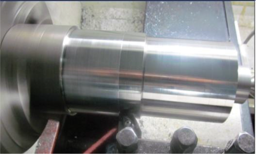
The photos of turning 300 M steel.

By single factor experiment, we know the influence regularity of the feed rate f, cutting speed v, depth of cut a _p , and corner radius r on the rough surface, as shown in Figure 2 to Figure 5.

Figure 2:

The influence of feed rate on surface roughness (v = 100 m/min, r = 0.8 mm, and a _p = 0.2 mm).

In Figure 2, the surface roughness of two kinds of cutting tools is strictly an increasing trend with the increase of feed rate, which illustrates that feed rate has a great influence on surface roughness. In Figure 3, when carbide tools were used to cut 300 M steel in the speed of 60 m/min~120 m/min, the surface roughness increases along with the increase of speed, but in the speed of 120 m/min~ 250 m/min, the surface roughness decreases with the increase of the speed, which illustrates that v = 120 m/min is a critical value when carbide tools were used to cut 300 M steel. The result has a certain reference value in the actual production and processing. When 300 M steel was cut by a ceramic cutting tool, the surface roughness reduces with the cutting speed increasing, but according to the change in Figure 4, we can see that the cutting depth effect on the surface roughness is less. Figure 5 shows the corner radius influence on surface roughness as when carbide cutting tools were used, the surface roughness decreases with corner radius increasing. But the surface roughness is least when r = 0.8 mm using ceramic cutting tool.

Figure 3:

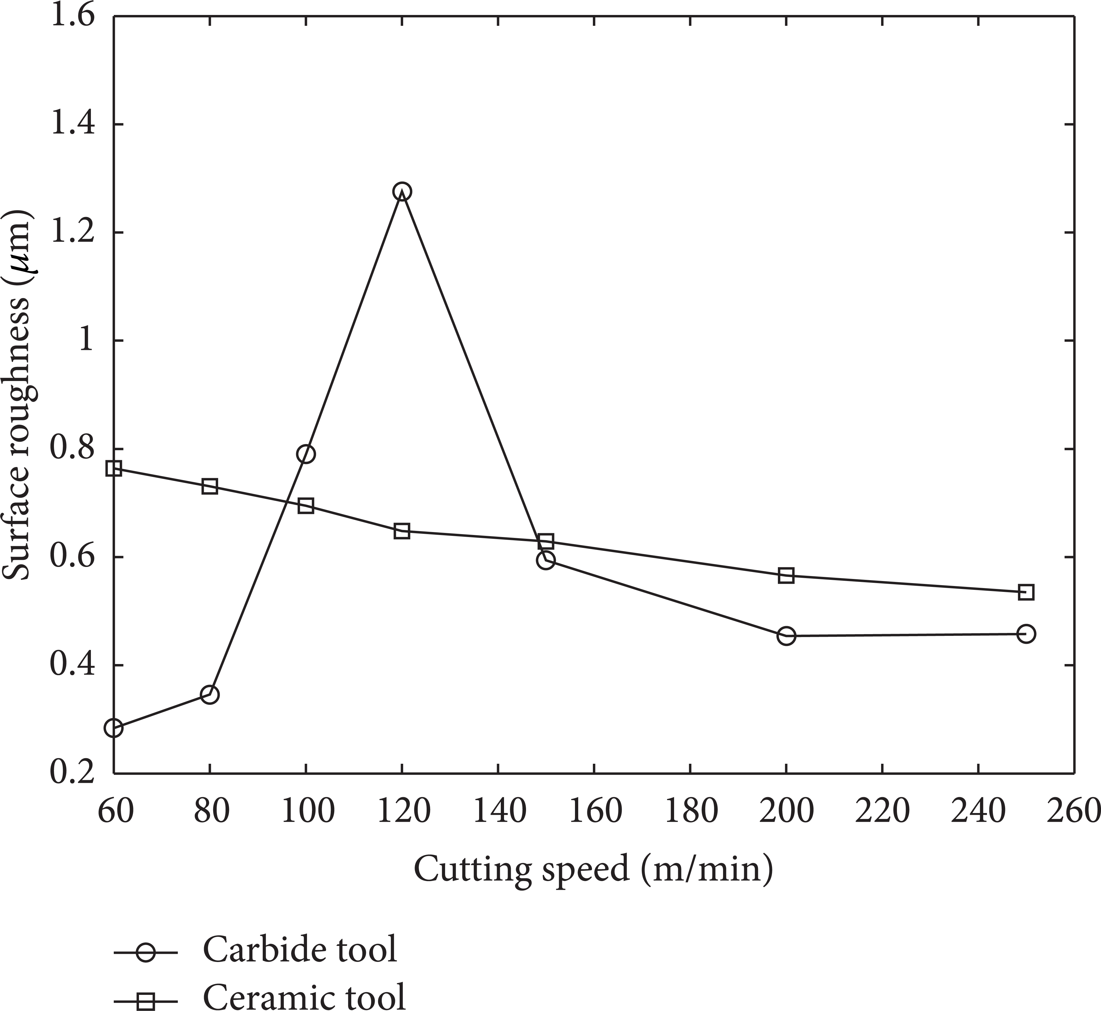
The influence of cutting speed on surface roughness (f = 0.1 mm/r, r = 0.8 mm, and a _p = 0.2 mm).

Figure 4:

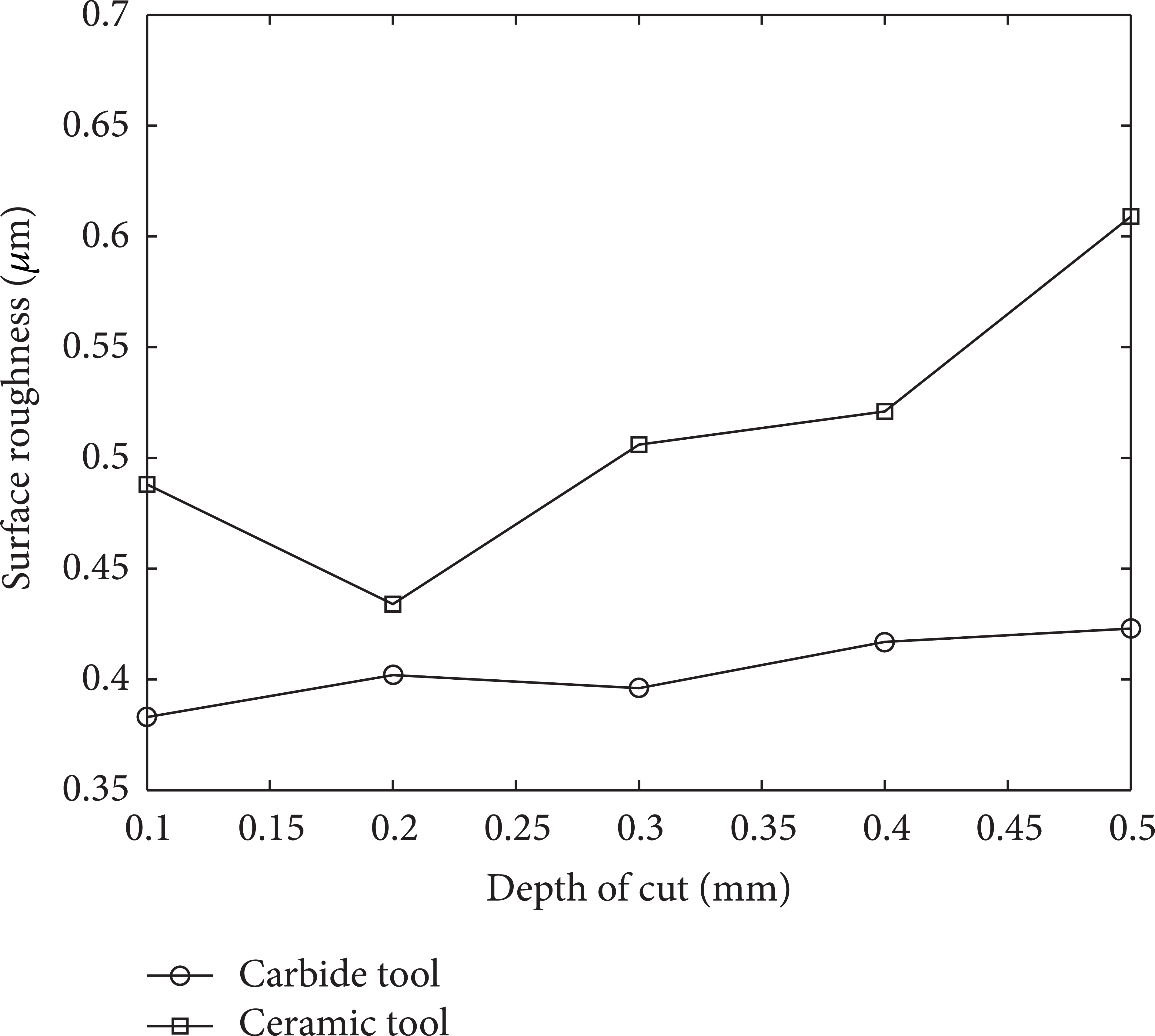
The influence of depth of cut on surface roughness (v = 100 m/min, r = 0.8 mm, and f = 0.1 mm/r).

Figure 5:

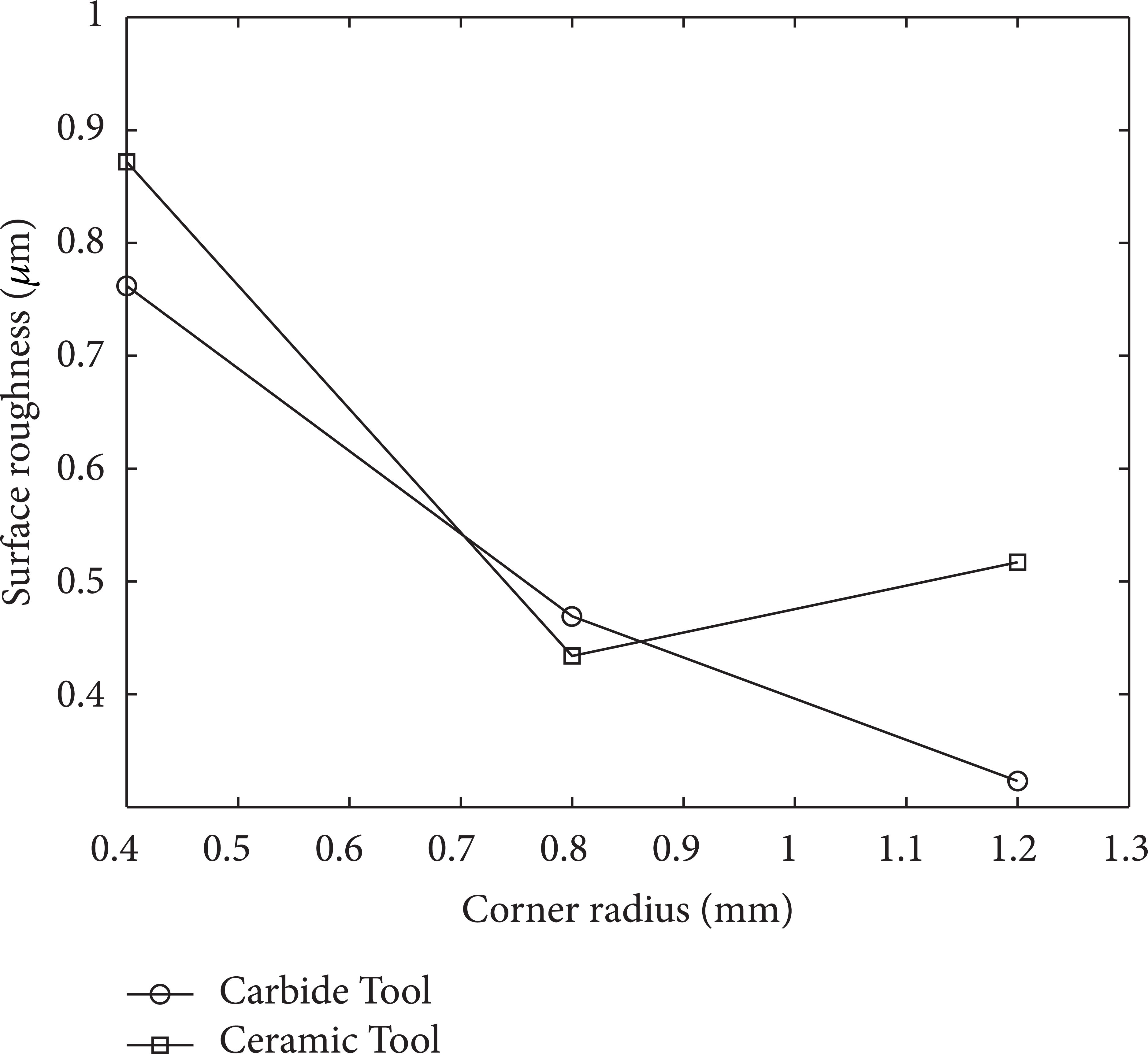
The influence of corner radius on surface roughness (v = 100 m/min, a _p = 0.2 mm, and f = 0.1 mm/r).

3. The Orthogonal Test of the Surface Roughness

The cutting tool of the test is PM4225 produced by the Sandvik Company, and other parameters unchanged, corner radius respectively changed from 0.4 mm to 1.6 mm. The four-factor and four-level orthogonal tests are done, respectively, regarding feed rate (f), cutting speed (v), depth of cut (a _p ), and corner radius (r) as the four variables. The orthogonal table of four factors and four levels (4⁵) is shown in Table 2.

Table 2:

Variable level.

Level	Cutting speed v (m/min)	Cutting depth a p (mm)	Corner radius r (mm)	Feed rate f (mm/r)
1	60	0.20	0.4	0.20
2	70	0.30	0.8	0.16
3	80	0.40	1.2	0.13
4	90	0.50	1.6	0.10

3.1. The Range Analysis of the Test Result

The surface roughness is measured twice and the average is taken as the result value. The analysis results are shown in Table 3.

Table 3:

The test results.

Number	A	B	C	D	Ra
	v (m/min)	ap (mm)	r (mm)	f (mm/r)	(µm)
1	1	1	1	1	1.864
2	1	2	2	2	1.084
3	1	3	3	3	0.398
4	1	4	4	4	0.272
5	2	1	3	4	0.365
6	2	2	4	3	0.345
7	2	3	1	2	0.901
8	2	4	2	1	1.355
9	3	1	4	2	0.449
10	3	2	3	1	0.852
11	3	3	2	4	0.356
12	3	4	1	3	0.682
13	4	1	2	3	0.489
14	4	2	1	4	0.777
15	4	3	4	1	0.691
16	4	4	3	2	0.613
I	3.618	3.167	4.224	4.281
II	2.966	3.058	3.284	3.047
III	2.339	2.346	2.228	1.914
IV	2.57	2.922	1.757	1.77
R	1.279	0.821	2.467	2.511

In Table 3, IV is the value of the maximum minus the minimum and R is the average value of each factor. We can conclude that the factors affecting the surface roughness from primary to secondary are D > C > A > B and that the most important factor is feed rate factor, while the second and third important factors are corner radius and cutting speed, respectively, and the depth of cut is minimum factor.

3.2. Establishing the Surface Roughness Model of Orthogonal Test

3.2.1. The Theoretical Mathematical Model

According to the actual need of turning, feed rate, cutting speed, corner radius, and depth of cut are regarded as variables to establish the prediction model of the surface roughness. Between surface roughness and cutting parameters there exists the complex exponential relationship, which can be expressed as follows:

$R_a=C{V}^k{a}_p^m{r}^n{f}^l.$

(1)

In formula (1), R _a is the surface roughness, C is the correction factor which is determined by the processing material and cutting conditions, and a _p is depth of cut. r is corner radius; f is feed rate; and k, m, n, and l are the index of each variable which is undetermined. We take the logarithm for both sides of formula (1) and the results are shown as follows:

$\begin{array}{c}\text{lg}{R}_a=\text{lg}c+k\text{lg}V+m\text{lg}{a}_p+n\text{lg}r+l\text{lg}f,\\ \text{order}\hspace{0.17em}\hspace{0.17em}y=\text{lg}{R}_a,\hspace{1em}\hspace{1em}a=\text{lg}c,\hspace{1em}\hspace{1em}{x}_{\mathrm{1}}=\text{lg}V,\\ x_{\mathrm{2}}=\text{lg}{a}_p,\hspace{1em}\hspace{1em}{x}_{\mathrm{3}}=\text{lg}r,\hspace{1em}\hspace{1em}{x}_{\mathrm{4}}=\text{lg}f,\\ \text{Then}\hspace{0.17em}y=a+k{x}_{\mathrm{1}}+m{x}_{\mathrm{2}}+n{x}_{\mathrm{3}}+l{x}_{\mathrm{4}}.\end{array}$

(2)

The multiple linear regression equation is established as follows:

$\begin{array}{l}{y}_{\mathrm{1}}={\beta }_{\mathrm{0}}+{\beta }_{\mathrm{1}}{x}_{\mathrm{11}}+{\beta }_{\mathrm{2}}{x}_{\mathrm{12}}+{\beta }_{\mathrm{3}}{x}_{\mathrm{13}}+{\beta }_{\mathrm{4}}{x}_{\mathrm{14}}+{\epsilon }_{\mathrm{1}},\\ y_{\mathrm{2}}={\beta }_{\mathrm{0}}+{\beta }_{\mathrm{1}}{x}_{\mathrm{21}}+{\beta }_{\mathrm{2}}{x}_{\mathrm{22}}+{\beta }_{\mathrm{3}}{x}_{\mathrm{23}}+{\beta }_{\mathrm{4}}{x}_{\mathrm{24}}+{\epsilon }_{\mathrm{2}},\\ ⋮\\ y_{\mathrm{16}}={\beta }_{\mathrm{0}}+{\beta }_{\mathrm{1}}{x}_{\mathrm{161}}+{\beta }_{\mathrm{2}}{x}_{\mathrm{162}}+{\beta }_{\mathrm{3}}{x}_{\mathrm{163}}+{\beta }_{\mathrm{4}}{x}_{\mathrm{164}}+{\epsilon }_{\mathrm{16}}.\end{array}$

(3)

In the above formulas, ε _i is the test deviation of the random variable. The above equation can represented in matrix form as Y = Xβ + ε:

$\begin{array}{c}Y=\left[\begin{array}{c}{y}_{\mathrm{1}}\\ y_{\mathrm{2}}\\ ⋮\\ y_{\mathrm{16}}\end{array}\right],\hspace{1em}\hspace{1em}\beta =\left[\begin{array}{c}{\beta }_{\mathrm{0}}\\ {\beta }_{\mathrm{1}}\\ ⋮\\ {\beta }_{\mathrm{4}}\end{array}\right],\hspace{1em}\hspace{1em}\epsilon =\left[\begin{array}{c}{\epsilon }_{\mathrm{1}}\\ {\epsilon }_{\mathrm{2}}\\ ⋮\\ {\epsilon }_{\mathrm{16}}\end{array}\right],\\ X=\left[\begin{array}{ccccc}\mathrm{1}& x_{\mathrm{11}}& x_{\mathrm{12}}& x_{\mathrm{13}}& x_{\mathrm{14}}\\ \mathrm{1}& x_{\mathrm{21}}& x_{\mathrm{22}}& x_{\mathrm{23}}& x_{\mathrm{24}}\\ ⋮& ⋮& ⋮& ⋮& ⋮\\ \mathrm{1}& x_{\mathrm{161}}& x_{\mathrm{162}}& x_{\mathrm{163}}& x_{\mathrm{164}}\end{array}\right].\end{array}$

(4)

Expression can be expressed in the form of y = b₀ + b₁x₁ + b₂x₂ + b₃x₃ + b₄x₄.

Among them, b₀, b₁, b₂, b₃, and b₄ are regression coefficients.

3.2.2. Establishing the Model

Using regress function of the MatLab software in the regression analysis, regression coefficient b is obtained as follows: $b={\left[\begin{array}{ccccc}1.5123& -0.2845& -0.0728& -0.6102& 1.4832\end{array}\right]}^T$ .

The predictive model of the surface roughness is obtained as follows: R _a = 32.5312V^−0.2845a _p ^−0.0728r^−0.6102f^1.4832.

3.2.3. Significance Test of Regression Model

By the data regression analysis functions of excel, variance analysis table is obtained and shown in Table 4.

Table 4:

Variance analysis table of prediction model.

Stem	Freedom	Squares	Mean square	F	F 0.05	R 2
Model	4	0.7471	0.1868	23.9764	3.36	0.8971
Residuals	11	0.0857	0.0078
Total	15	0.8328

According to the rcoplot function of MatLab software to regression analysis, its residual plot shows the fourteenth point is outliers, and the residuals are shown in Figure 6. In order to make its models more accurate, exclude outliers and do the regression analysis again, the regression coefficient b is obtained again as follows: $b={\left[\begin{array}{ccccc}2.2290& -0.5798& -0.0436& -0.5080& 1.6728\end{array}\right]}^T$ .

Figure 6:

Regression residual plots.

The prediction model is obtained again as follows: R _a = 169.4338V^−0.5798a _p ^−0.0436r^−0.5080f^1.6728.

By the data regression analysis functions of excel, regression analysis table is obtained and shown in Table 5.

Table 5:

Variance analysis table of prediction model.

Stem	Freedom	Squares	Mean square	F	F 0.05	R 2
Model	4	0.7702	0.1926	36.5793	3.48	0.9360
Residuals	10	0.0526	0.0053
Total	14	0.8229

The two variance analysis tables show that F is much larger than the value of F_0.05, so the two regression models are highly significant. But the second model excludes outliers, and the coefficient of determination R² and F must be greater than the value of the first model, so the second model was selected as a predictor model of the surface roughness.

4. The Single Factor Experiment of Residual Stress

The equipment and material of experiment are shown above. The cutting tool is CNGA A65 series produced by kyocera. After the cutting test, the parts are cut down by the method of wire cutting to do the residual stresses experiments. The residual stresses experiments are done with the X-350A X-ray stress test system (as shown in Figure 7) and XF-1 type electrolytic polishing machine, Micrometer, and so on. In order to research the workpiece surface residual stresses, we need not only to know the surface residual stress distribution, but also to measure the residual stress distribution along the depth direction.

Figure 7:

Residual stress measurement device in the test.

X-ray stress tester can only measure residual stress on the surface of the sample. If we want to measure the change of the residual stress along the depth direction, we need to use electrolytic etching method to strip and test the sample layer by layer; finally, we got the residual stress distribution along the depth direction. The surface of the sample is stripped by XF-1 electrolytic polishing machine.

4.1. Experimental Results and Analysis

After testing, the residual stress data is obtained and shown in Figure 8.

Figure 8:

Cutting speed impact on residual stress layer depth distribution (a _p = 0.2 mm and f = 0.1 mm/r).

As can be seen from Figure 8(a) (the circumferential stress) and from Figure 8(b) (the radial stress), when the cutting speed increases, the surface residual stress changes from the compressive stress to the tensile stress. This is due to the impact of thermoplastic deformation. When the speed increases, the heat generated by the cutting area increases, but most of the heat is taken away by the chip and the heat flew to the workpiece reduces. The surface Contraction is subject to the constraints of the inner layer thus formed the residual tensile stress in the surface. As the speed increasing, the maximum residual compressive stress of the surface increases and the residual stress layer thickness is deeper. In the place from the surface about 15 um, the gradient of the residual stress reaches a maximum, so that the residual compressive stress reaches a maximum. When the depth is up to 50 um, the residual stress basically reaches the original stress state. It means that the plastic deformation of workpiece metamorphic layer end.

Figure 9(a) (circumferential stress) and Figure 9(b) (radial stress) show the different feed rate influence on the residual stress. It can be seen from Figure 9(a) that the residual tensile stress of the surface increases with the increase of the cutting speed. This is because the cutting force and cutting temperature increase with the feed rate increasing, but it has not reached phase transition temperature. At this time, the mechanical and thermal stresses dominate, so the residual stress in the surface layer shows an increasing trend. From Figures 9(a) and 9(b) it can clearly be seen that the residual compressive stress along the layer depth direction increases with the feed rate increasing. This is because cutting heat increases the impact of the inner metal layer when the cutting temperature increases. Therefore, the maximum residual compressive stress occurs at a deeper layer. The active layer depth of circumferential stress is in the range of 5–15 um, and the active layer depth of radial stress is in the range of 5–15 um. There is a great difference between the radial and circumferential stresses. But the residual stress changes to the original stress state at about 75 um. This indicates that the plastic deformation of metamorphic layer ends at this area of workpiece.

Figure 9:

Feed rate impact on residual stress layer depth distribution (a _p = 0.2 mm and v = 100 m/min).

The influence of depth of cut on surface residual stress is so complex that it has not been determined. Those factors that can cause plastic deformation and cutting temperature to change during machining will have an effect on residual stress. The influence of depth of cut on the cutting temperature is very small, but its effect on the plastic deformation is the current focus of the controversy. Some researchers think that although the cutting force increases when depth of cut increases, the cutting force on the unit length of the blade has no obvious change [6, 7]. Other researchers think that the volume and section of the cutting layer metal increase with the cutting force increasing that makes the plastic deformation range and deformation degree of the cutting edge front increase [8, 9]. As the related mechanism research is not enough, the influence of cutting depth on residual stress cannot be theoretically and qualitatively analyzed. From Figure 10, we know that the 300 M steel cutting surface residual stress and depth of cut have a certain relationship.

Figure 10:

Depth of cut impact on residual stress layer depth distribution (f = 0.1 mm/r and v = 100 m/min).

5. Conclusion

In summary, we can draw the following conclusions.

1. Through the orthogonal experiment of cutting the 300 M steel, the prediction model on surface roughness is established (with the same blade and hardness) when v _c is 60~90 m/min, a _p is 0.2~0.5 mm, and f is 0.1~0.2 mm/r. The model passes the experiments and has the high machining accuracy, which provides powerful basis for later production processing.

2. By selecting different cutting parameter values in the processing, different residual stress values of workpiece machined surface can be obtained. Because of the fact that the generation of residual stress is the result of a combination of factors, the residual stresses may be the compressive stress or tensile stress and their sizes are not the same. When one factor among the other factors plays a leading role, it shows the corresponding surface residual stress. For 300 M ultrahigh strength steel, selecting low speed and low feed as cutting parameter can make the processed surface of the workpiece suffer compressive stress which is good at improving the fatigue life of workpieces.

3. The distribution regularity of residual stress layer depth is as follows: (1) with the speed increasing, the residual stress of machined surface changes from compressive stress to tensile stress, the maximum value of residual compressive stress of the subsurface layer increases, and the effecting depth of residual stress decreases and (2) with the feed rate increasing, the value of the surface residual tensile stress increases, the maximum value of residual compressive stress of the subsurface layer increases, and the effecting depth of residual stress increases. So the machined surface residual stress and the subsurface residual stress have a certain relationship with the cutting depth.

Conflict of Interests

The authors declare that they have no conflict of interests regarding the publication of this paper.