Simplified Pedestrian Tracking Filters with Positioning and Foot-Mounted Inertial Sensors

Abstract

Pedestrian tracking is one of the bases for many ubiquitous context-aware services, but it is still an open issue in indoor environments or when GPS estimations are not optimal. In this paper, we propose two novel different data fusion algorithms to track a pedestrian using current positioning technologies (i.e., GPS, received signal strength localization from Wi-Fi or Bluetooth networks, etc.) and low cost inertial sensors. In particular, the algorithms rely, respectively, on an extended Kalman filter (EKF) and a simplified complementary Kalman filter (KF). Both approaches have been tested with real data, showing clear accuracy improvement with respect to raw positioning data, with much reduced computational cost with respect to previous high performance solutions in literature. The fusion of both inputs is done in a loosely coupled way, so the system can adapt to the infrastructure that is available at a specific moment, delivering both outdoors and indoors solutions.

1. Introduction

The need to know where a person is dates back to centuries ago; in the last decades, traditional maps and compasses have been increasingly replaced by navigation assistance systems. At the beginning of this century the use of the global position system (GPS) became popular, democratizing the availability of location estimation for many civilian services. This system, nowadays integrated in every smartphone, may be not good enough for many applications, such as those involving stand-alone pedestrian localization. This is due to the GPS accuracy, within the range of 5–20 m for urban/indoor environments, where typical errors (in the order of 2–5 meters) are increased due to the presence of local error sources (e.g., multipath, signal attenuation, and diffraction). Current generations of high sensitive GPS receivers may be good enough for some indoor applications [1], but their performance rapidly degrades with the number of walls and depends on their materials. Therefore, the position error is often too large and the system's availability is insufficient especially for deep indoor environments. Research on personal localization and navigation systems has attracted a lot of attention since the Federal Communication Commission (FCC) published the Enhanced 911 (E-911) implementation requirements in 1999 [2]. Many location based services (LBS) have been developed since then, and a wide offer of applications is nowadays available in the most popular application stores [3]. From intervention tools for emergencies or visually impaired guidance to tourism guides augmented with context-aware recommendations [4], all these applications need to track their users. Obviously, the accuracy requirements vary depending on the service leitmotif.

Pedestrian localization presents some challenges when compared to car or robot tracking. On the one hand, the movements of vehicles are more predictable—as they usually move along the predefined paths of the road network, while pedestrians move freely, changing their path unexpectedly due to obstacles or on-the-spot decisions [5]. On the other hand, vehicles and robots may have many sensors attached, if needed. However a pedestrian will reject wearing a sensor that hinders his movements due to weight, bulkiness, and so forth. Finally, the walking characteristics not only differ from individual to individual, but also depend on factors difficult to characterize or estimate, such as state of mind, type of shoes or type of pavement.

Previous works have addressed the problem of pedestrian tracking in two different ways: (a) relying on supporting infrastructure or (b) using wearable sensors. Solutions in the latest group have applied traditional localization methods based on the information provided by inertial sensors. The use of inertial sensors has privacy advantages over other technologies for localization and tracking, such as camera networks. Their low weight makes it possible to integrate them in wearable forms (shoes, mobile phones, etc.) and the processing of their data requires low computational capabilities, being suitable for real-time applications.

Those systems are usually called strap-down systems, since the sensors used are strapped to the body that is going to be tracked. There are two main approaches to deal with the problem of estimating the position of a person using the information provided by inertial sensors: (step based) dead reckoning (DR) and inertial navigation systems (INS). DR is based on the analysis of the periodic signals that result from the dynamics of walking in order to count steps. This enables us to calculate the traversed distance by using an estimation of the step length. In addition, a magnetic compass or a gyroscope is employed to estimate the heading of the direction of walking, in order to project the traversed distance in the horizontal plane. With respect to the INS method, the measurements of the accelerometer are double integrated taking into account platform orientation according to compass and/or gyroscopes, to get an estimation of the position change with time. However, the influence of the errors of inertial sensors on the position estimation makes it very difficult to achieve continuous accurate localization using stand-alone inertial navigation systems, as the inherent integration of both approaches tends to make the error increase along time. The sensors for pedestrian localization are usually low-grade sensors, which means that the errors in the measurements have a significant influence over the achieved results (accelerometer and gyroscope errors make the position error grow over the time [6]), unless some correcting/aiding technique is applied, such as zero velocity updates (ZVU) [7]. ZVU (i.e., controlling the instants when the foot is placed on the ground, ad thus the velocity and acceleration are zero) are commonly used in pedestrian positioning systems. In order to apply such technique, the inertial sensors must be in the feet.

The sources of inertial sensor errors and their influence over the estimation of the pedestrian position are analyzed in [8–10]. To reduce the impact of these growing errors, several aiding strategies have been proposed [8]. Neither of them achieves a general solution that provides enough accuracy for pedestrian tracking, so fusion with other sensors with bounded error statistics is often considered. The fusion of the different aiding sensors with the inertial information is made using techniques such as particle filters [11–13] or Kalman filters. For instance, the algorithm in [11] attains an average error in the order of 1.5 meters using particle filters to fuse belt-mounted INS and Wi-Fi RSS positional measurements, while the proposal in [12], with a very similar approach, achieves an error in the order of 4.5 m. The similar strategy in [13] provides an average error in the order of 1 m. In the two later cases, map-aiding was also implemented.

The algorithms proposed in this paper would be implemented in a mobile device (i.e., smartphone). ZVU are used whenever the foot is detected on the ground (which occurs periodically as the pedestrian walks). For this reason, the system includes a detector to accurately determine the instants when the foot of a user is placed on the floor. Moreover, the inertial system is aided with positioning measurements taken from an external localization system, which could be either a GPS in outdoor environments or a wireless positioning system in indoor environments. Typically those indoor wireless positioning systems perform location estimation from RSS measurements of the underlying communication technologies (i.e., Wi-Fi, Bluetooth, or ZigBee motes) [14]. Many existing solutions are based on Kalman filters (KF), which provide a reduced computational load with respect to particle filters. Some of those works propose a complementary Kalman filter that estimates the errors of the position, velocity, acceleration, and the bias of the sensors, subtracting them from the states and measurements for the integration. Approaches such as the ones described in [15, 16] include an inertial navigation system that works in parallel with that complementary KF. In particular, the proposal in [16] focuses specifically in the detection of the ZVU intervals, although very limited experimental results support the design.

In [17], the positioning system is based on processing the RSS measurements from RFID tags in a tightly coupled way. The obtained average error is 1.35 m along 4 trajectory scenarios of 600, 550, 520, and 1000 m. of length, respectively. Moreover, GPS measurements are integrated in outdoors environment using a loosely coupled complementary Kalman filter, and magnetometer data is also used to aid in indoor navigation in [18] achieving results with an average error around 2 m in a 300 m long trajectory.

In this paper, a novel extended Kalman filter (EKF) and a simplified complementary Kalman filter (KF) are proposed; both filters enable the fusion of the position computed through one or more inertial sensors with periodic position updates provided by a positioning solution based on wireless technologies (GPS or indoor positioning system). The fusion system includes some quite important simplifications of sensor and movement modeling with respect to those existing in literature (specifically on the Foxlin's contribution [15], which inspires one of the proposed solutions). In the results section it is shown how, even with those simplifications, the system maintains a high accuracy, being robust enough for many typical localization applications. The main contribution of our approach is the very small computational load and battery consumption introduced by the filter, a feature of paramount importance in resource and energy-constrained wearable applications. The fusion of both inputs is done in a loosely coupled way, so the system can adapt to the infrastructure that is available at a specific moment. Additionally, the solution is ubiquitous, as it can work in indoor environments using the information from wireless technologies or outdoors, using a GPS receiver.

The paper provides an overview of both approaches, performing a comparative analysis of their quality. Sections 2 and 3 describe the models assumed for the problem formulation. In particular, Section 2 describes the pedestrian movement in terms of the typical signals measured by inertial and positioning systems, while Section 3 is centered on the description of the errors coming from typical wearable sensors. Afterwards, Section 4 includes the derivation of the two different proposed filtering solutions. Performance is analyzed in Section 5, comparing it with other solutions, especially from the point of view of their accuracy and computational load. Finally, Section 6 contains some conclusions and limitations on the applicability of these techniques.

2. Pedestrian Movement Modeling

Human walking is a process of bipedal locomotion in which the weight of the moving body is supported by one leg, while the other moves forward (i.e., the center of gravity swaps between the left and the right side of the body) in an alternate sequence necessary to cover a distance [19]. A gait cycle can thus be defined. This gait cycle, which happens to be reasonably consistent among different individuals, is mainly composed of a stance phase during which one foot is in contact with the ground and a swing phase, during which the foot is in the air. These two phases can be easily distinguished when analyzing the measurements gathered from different inertial sensors mounted on the pedestrian's feet. In addition, pretty short heel strike and foot lift-off phases can be detected along the gait, when the highest acceleration appears, but with reduced effect on the complete traversed distance. In [20], it is proposed an acceleration-based strategy to count the steps that a person takes (which is particularly interesting for dead-reckoning systems). Authors only care about the periodic shape of the acceleration signal, regardless of the result of its double integration. In inertial navigation, the focus is on the information that is provided by the integration of the acceleration signal, representing the velocity applied in the step (simple integration) and the position (double integration).

In order to analyze a pedestrian movement, the measurements from the different sensors from an experimental IMU have been considered. These sensors are raw measures from two orthogonal accelerometers, mounted on a plane roughly parallel to the sole of the foot, along foot (longitudinal) and orthogonal to its axis (transversal), and a heading “sensor” based on integration of IMU gyroscopes and magnetometer. Heading derivation is performed within the IMU using their proprietary algorithms. These will be the same measures to be used in our simplified filters. In particular, the MTx IMUs from Xsens have been used [21] for the experimental part of this work (see Figure 1).

Figure 1

MTx sensor unit.

The IMU will be foot-mounted. The choice of the foot as the position of the sensor is due to the fact that our processing will make use of ZVU, which can be applied to reset the drifts accumulated in the filter due to the errors of the measured signals.

For this setting, the two main reference systems for inertial navigation will be as follows.

• (i)

  Inertial reference system $(I)$ : it is an earth-fixed right handed Cartesian coordinate system, external to the pedestrian, with three orthogonal axes. $X_I$ axis points towards the local magnetic North, $Z_I$ axis points up, and $Y_I$ axis points West. The pedestrian trajectory will be tracked in these coordinates.

• (ii)

  Foot reference system $(F)$ : the orthogonal axes of this coordinate system are defined by the orientation of the three accelerometers embedded in the IMUs. This coordinate system is important as the acceleration measures are initially referred to it. In this coordinate system, $X_F$ points to the longitudinal direction of the foot, $Y_F$ points horizontally to the left of the foot (transversal), and $Z_F$ points up (following the direction of the leg).

• (iii)

  Body reference system (B): this reference system can be defined from the rotation of foot reference system so that $X_B$ points to the longitudinal direction of the foot, but in the horizontal plane. Then, $Y_B$ points to the left of the foot (transversal), being equivalent to $Y_F$ , and $Z_B$ points up (normal to horizontal plane). This reference system is not affected by the pitching movement of the foot along the stride.

Figure 2 shows measurements taken along several strides during a typical constant course movement of a pedestrian. In this specific case, each stride lasts around 50 samples or 1 second, since the sample frequency is 50 Hz (it must be noted that each stride of the signal corresponds to one left and one right foot step). Around 40% of the time of the step corresponds to the stance phase (zero acceleration, zero rate of turn, constant heading) and there are several peaks in the different phases of the movement:

• (i)

  a quite deterministic longitudinal acceleration at the beginning of the step and a deceleration at its end: this acceleration is measured by the longitudinal accelerator, being therefore, expressed along $X_F$ axis;

• (ii)

  a much smaller and less deterministic transversal acceleration swing (measured in either $Y_F$ or $Y_B$ axis), coupled with rate of turn and heading changes as the foot moves along the step. Note that the maximum heading excursion along the step is lower than 15°, for short times at the beginning of each step. This behavior is pretty dependent on pavement and shoes.

Figure 2

Along-time measures (a) Transversal acceleration. (b) Longitudinal acceleration. (c) Heading provided by the IMU.

When the pedestrian performs a maneuver, the resulting signals change, causing the following situations.

• (i)

  When the pedestrian stops, all acceleration signals become zero and heading becomes constant. Additionally, depending on the last foot in movement, the last step might be shorter, and therefore the associated longitudinal acceleration might be smaller.

• (ii)

  Usually, at the beginning or end of pedestrian movements the body velocity increases or decreases. This typically has to do with smaller acceleration, although in those situations the movement is not so deterministic, as the balance of the body and movement is not perfect.

• (iii)

  Along turns, typically, the heading tends to rapidly change to reach the new course.

The following key ideas might be derived from these foot mounted IMU signals.

• (i)

  There are distinct modes of longitudinal movement for the feet: stopped, quite fast acceleration at the beginning and end of the step, and slow acceleration changes along the step.

• (ii)

  Lateral movement can be seen as the movement of the pedestrian body with some additional error introduced by the lack of balance of the person along each step.

Although it is perfectly possible that a person moves laterally, this kind of movement is not usual while walking (but it could be typical for some other kind of activities such as dancing or playing tennis). Additionally, the presented models will demand changes for the running movement, where the heading excursions and duration of the different stride phases will be different. Our movement models and the proposed processing methods, which are based on them, are not well suited for these other types of movements. A final consideration is that all our movement models assume that walking is performed over a flat surface.

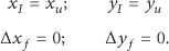
3. Measurement Modeling

Next we will mathematically describe the sensors that have been considered and the models of their errors, detailing the notation of the variables that characterize the movement and the associated measurements. In addition to the terms included in (1) to (3), all sensors include noise error terms, which are not considered here for the sake of simplicity. Of course, the proposed processing systems will take into account the presence of those noise terms in their (Kalman filter) measurement models.

Position sensors may be of different kinds, for indoor and outdoor applications. For indoor applications it is frequent to use RSS-based positioning systems. Those systems suffer from quite a complex range of errors due to multipath and propagation, leading to measures that have typically (time and space) varying bias and noises. In our simplified approach, we will assume that the positioning system has negligible bias and constant noise statistics. Therefore, we will have

$$\begin{array}{cc}& E\left\{x_m\right\}=x,\hspace{1em}\hspace{1em}E\left\{y_m\right\}=y,\end{array}$$

(1)

where $(x,y)$ is the current actual position of the pedestrian and $(x_m,y_m)$ is the associated measurement. Here, and in the rest of equations, $E\{·\}$ is the expectation operation. Both actual position and position measures are taken in the inertial reference system. The same model might be used with differential GPS positioning system measurements in outdoor applications, although different statistical (noise covariance) parameters should be used in this case in the tracking filters.

The accelerometer sensor measures the force applied to a body in a specific direction and converts it into acceleration (in m/s²). The longitudinal (along foot) and transversal components are used to track the 2D movement. In our systems, acceleration is measured in the foot reference system and translated into the body reference system using the attitude of the accelerometer estimated by the inertial system. Thus the input measures to our filters will be defined in the body reference frame. This rotation of the acceleration corrupts the longitudinal acceleration measurement along the stance by the time-varying projection of gravity (this term is smaller than 0.5 m/s² for a walking pedestrian but could be larger if he is running). Both acceleration $(a)$ measurements are typically considered to contain an offset error due to technological limitations [1, 9, 10]. So we assume an almost constant offset in both coordinates:

$$\begin{array}{cc}& E\left\{a_{Lm}\right\}=a_L+\Delta a_L,\hspace{1em}\hspace{1em}E\left\{a_{Tm}\right\}=a_T+\Delta a_T,\end{array}$$

(2)

where $a_L$ is the real longitudinal acceleration, $a_T$ is the real transversal acceleration, m subindex stands for measure, and Δ stands for offset in the measurement. Therefore $a_{Lm}$ would be the measurement of the longitudinal acceleration and $\Delta a_T$ would be the offset in the measure of the transversal acceleration. The same notation will be used along the following equations. It should be emphasized again that this is a very rough model of the error, as the pitching movement of the foot along the stride will make the projection of those biases not constant in time, especially due to the projection of gravity in the longitudinal accelerometer. In our proposal, we are investigating if neglecting the effect of this important error source enables a simpler tracking system without compromising tracking accuracy and stability.

The heading $(\psi )$ measurements are obtained by the combination of the measurements gathered from various sensors included in the IMU, such as accelerometers, gyroscopes, and magnetometers. This processing stabilizes the measurements from the different sensors, being embedded in the IMU hardware and computed in real time. The result is the measured heading angle ( ${\psi }_m$ , in radians) describing the direction of the pedestrian movement, which is affected by a small error ( $\Delta \psi$ ); this error may be assumed to be almost constant:

$$\begin{array}{cc}& E\left\{{\psi }_m\right\}=\psi +\Delta \psi .\end{array}$$

(3)

This model is not so clear, especially taking into account the time correlation of the errors induced by the IMU processing methods and the use of magnetometer measures which can be corrupted due to the presence of metallic or electronic objects in the environment, a circumstance that is quite usual in indoor environments. From our experience with indoors heading measures, we may state that $\Delta \psi$ tends to change along time at different rates quite slowly when the pedestrian follows constant heading paths or stops and much faster along pedestrians turns. This will demand specific means to improve the processing in our filter.

It should be noted that actual foot accelerations can be higher than 5 G and specially and turn rates may be way over 300 degrees/second, which are the default dynamic ranges of the IMUs used in our deployment. Together with the quite low 50 Hz sampling rate, such hardware limitations can seriously reduce the accuracy (for instance in sharp turns) of INS systems based on those sensors. Our approach is quite robust against these problems, as will be seen in the results section, due to its capability to estimate the accumulated inertial integration error terms, unobservable from inertial measures. But, of course, better sensors could allow much improved overall solution quality.

4. Proposal of Alternative Fusion Approaches for Position and Accelerometer Data Fusion

Two different filters for pedestrian tracking are proposed and compared in this work. The first is an extended Kalman filter (EKF) that considers in the state variables the offsets of the measurements’ bias (both for accelerometers and heading). The other filter is a complementary Kalman filter (KF) inspired on the filters suggested by Foxlin [15].

Our filters use simplified 2D kinematic models with respect to those in the literature, not trying to estimate gyro bias and neglecting the importance of vertical acceleration bias in order to reduce overall computational load. Our complementary filter (second solution) estimates not only the actual dynamics of the pedestrian, but also some correction terms for the integration:

• (i)

  $\Delta x,\Delta y$ : offset in $X_I$ and $Y_I$ derived from the accumulative errors in the inertial system integration;

• (ii)

  $\Delta \left|v\right|$ : offset in the velocity magnitude, derived from the accumulative errors in the inertial system integration.

All filters will process 2D position measurements using a loosely coupled solution. This solution is chosen due to the fact that the system must run in several possible scenarios, with different 2D position sensors for indoor and outdoor applications and depending on the deployed positioning technologies available.

In the notations section there is a summary of the common notation that is used to define the variables of both filters.

In the following sections, the notation of the EKF/KF used in the book by Gelb et al. [22] has been used. So, the EKF/KF equations will be as follows.

• (i)

  Prediction:

  $$\begin{array}{cc}& {\overrightarrow{x}}_p=f\left({\overrightarrow{x}}_f\right),\\ P_p=F{P}_f{F}^T+Q,\end{array}$$

  (4)

where ${\overrightarrow{x}}_p$ is the predicted state estimate at current instant, ${\overrightarrow{x}}_f$ is the filtered estimate just after previous update, and $f(·)$ is the potentially nonlinear function that enables predicting the current state from the previous state. Meanwhile, $P_p$ is the covariance associated to ${\overrightarrow{x}}_p$ , $P_f$ is the covariance associated to ${\overrightarrow{x}}_f$ , F is the Jacobian matrix of $f(·)$ , and Q is the covariance matrix of the plant noise. During the prediction stages, the subindex p will always refer to current time prediction and the subindex f to previous update filtered estimate. We will not include any time index in the equations, in order to reduce its size to the minimum.

• (ii)

  Filtering (update):

  $$\begin{array}{cc}& K=P_p{H}^T{\left(H{P}_p{H}^T+R\right)}^{-\mathrm{1}},\\ {\overrightarrow{x}}_f={\overrightarrow{x}}_p+K\left({\overrightarrow{x}}_m-h\left({\overrightarrow{x}}_p\right)\right),\\ P_f=\left(I-KH\right)P_p,\end{array}$$

  (5)

where ${\overrightarrow{x}}_p$ is the predicted state estimate at current instant and ${\overrightarrow{x}}_f$ is the filtered estimate at the same instant, after the incorporation of the information in the current update, included in measurement vector $({\overrightarrow{x}}_m)$ . $h(·)$ is the potentially nonlinear projection function relating dynamic and bias states to Kalman measurements. Meanwhile, $P_p$ is the covariance associated to ${\overrightarrow{x}}_p$ , $P_f$ is the covariance associated to ${\overrightarrow{x}}_f$ , H is the Jacobian matrix of $h(·)$ , R is the covariance matrix of the measurement noise, and K is the Kalman gain matrix. During the filtering stages, both subindexes f and p will always refer to current time filtering and prediction. Subindex m will be used for input measurements at this time.

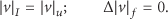
Next we will describe our proposed processing systems, first explaining the overall architecture and associated state vector (which will be always equivalent for predicted and filtered states) and then clarifying the form of the different components in (4) and (5). Subindex f will be used to denote filtered state components, while subindex p will be used for predicted state, as described above. The time instant they refer to will depend on the involved calculation being part of the prediction or filtering stage, as described in the previous paragraphs.

4.1. Centralized EKF

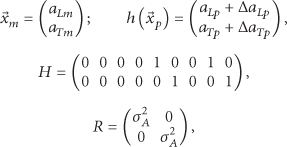
The first proposed filter is an extended Kalman filter, which may process three different kinds of measurements (using appropriate specifications of $h(·)$ and H):

• (i)

  position: $(x_m,y_m)$ , measured in the inertial reference frame;

• (ii)

  acceleration: $(a_{Lm},a_{Tm})$ , projected into the inertial reference frame;

• (iii)

  heading: ${\psi }_m$ ; it should be noted that this measurement is obtained from the IMU, which performs integration of gyroscope rates of turn to derive this value. The heading sensor will also be aided by the use of a compass.

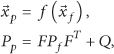
This EKF has the following associated state (described here for the filtered state):

$$\begin{array}{cc}& {\overrightarrow{x}}_f={\left[\begin{array}{ccccccccc}{x}_f& y_f& {\left|v\right|}_f& {\psi }_f& a_{Lf}& a_{Tf}& \Delta {\psi }_f& \Delta a_{Lf}& \Delta a_{Tf}\end{array}\right]}^T.\end{array}$$

(6)

The state variables are the position, velocity (expressed with its magnitude and heading angle), and acceleration vectors together with the offsets assumed in the measurements, that is, heading and acceleration offsets, assumed to be constant in our simplified error model. The idea of this filter is to jointly estimate the dynamic state of the pedestrian and the principal slowly changing components of the sensors errors. Those slowly changing offsets will be implicitly removed from the trajectory estimation, resulting in the mostly bias-free tracking of the pedestrian. The key to be able to do so is the observability of the offset terms, which is attained along time due to the presence of position measures, which finally allow their calibration and removal. Other error sources for the integration are assumed to have reduced impact in the output. In fact, the filter will estimate a set of offsets, which will not accurately describe the actual errors terms but will be able to calibrate the inertial equations leading to effective removal of induced positional biases.

4.1.1. Prediction Model

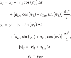
In this first proposed filter there are several potential modes of movement, related to the phases of each step. For the phases where the foot is moving, we assume a prediction of the position coordinates in the inertial coordinate system, following constant acceleration motion between samples for the position, circular motion for heading, and constant bias models. If the time between the current measure and the previous one is $\Delta t$ , we can approximate the associated state changes with time as follows:

$$\begin{array}{cc}& \left(\begin{array}{c}{x}_P\\ y_p\\ {\left|v\right|}_p\\ {\psi }_p\\ a_{Lp}\\ a_{Tp}\\ {\Delta \psi }_p\\ {\Delta a}_{Lp}\\ {\Delta a}_{Tp}\end{array}\right)={\overrightarrow{x}}_p=f\left({\overrightarrow{x}}_f\right)=\left(\begin{array}{c}{x}_f+{\left|v\right|}_f\cos \left({\psi }_f\right)\Delta t+\frac{\left[a_{Lf}\cos \left({\psi }_f\right)-a_{Tf}\sin \left({\psi }_f\right)\right]{\Delta t}^{\mathrm{2}}}{2}\\ y_f+{\left|v\right|}_f\sin \left({\psi }_f\right)\Delta t+\frac{\left[a_{Lf}\sin \left({\psi }_f\right)+a_{Tf}\cos \left({\psi }_f\right)\right]{\Delta t}^{\mathrm{2}}}{2}\\ {\left|v\right|}_f+a_{Lf}\Delta t\\ {\psi }_f+\frac{a_{Tf}\Delta t}{{\left|v\right|}_f}\\ a_{Lf}\\ a_{Tf}\\ {\Delta \psi }_f\\ \Delta a_{Lf}\\ \Delta a_{Tf}\end{array}\right).\end{array}$$

(7)

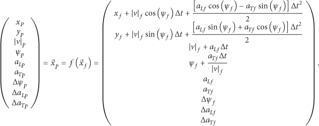
The Jacobian matrix of the prediction model (F in (4)) is

$$\begin{array}{cc}& F=\left(\begin{array}{ccccccccc}\mathrm{1}& \mathrm{0}& \cos \left({\psi }_f\right)\Delta t& F_{\mathrm{1,4}}& \frac{\cos \left({\psi }_f\right){\Delta t}^{\mathrm{2}}}{2}& \frac{-\sin \left({\psi }_f\right){\Delta t}^{\mathrm{2}}}{2}& \mathrm{0}& \mathrm{0}& \mathrm{0}\\ \mathrm{0}& \mathrm{1}& \sin \left({\psi }_f\right)\Delta t& F_{\mathrm{2,4}}& \frac{\sin \left({\psi }_f\right){\Delta t}^{\mathrm{2}}}{2}& \frac{\cos \left({\psi }_f\right){\Delta t}^{\mathrm{2}}}{2}& \mathrm{0}& \mathrm{0}& \mathrm{0}\\ \mathrm{0}& \mathrm{0}& \mathrm{1}& \mathrm{0}& \Delta t& \mathrm{0}& \mathrm{0}& \mathrm{0}& \mathrm{0}\\ \mathrm{0}& \mathrm{0}& \frac{-a_{Tf}\Delta t}{{\left|v\right|}_f^{\mathrm{2}}}& \mathrm{1}& \mathrm{0}& \frac{\Delta t}{{\left|v\right|}_f}& \mathrm{0}& \mathrm{0}& \mathrm{0}\\ \mathrm{0}& \mathrm{0}& \mathrm{0}& \mathrm{0}& \mathrm{1}& \mathrm{0}& \mathrm{0}& \mathrm{0}& \mathrm{0}\\ \mathrm{0}& \mathrm{0}& \mathrm{0}& \mathrm{0}& \mathrm{0}& \mathrm{1}& \mathrm{0}& \mathrm{0}& \mathrm{0}\\ \mathrm{0}& \mathrm{0}& \mathrm{0}& \mathrm{0}& \mathrm{0}& \mathrm{0}& \mathrm{1}& \mathrm{0}& \mathrm{0}\\ \mathrm{0}& \mathrm{0}& \mathrm{0}& \mathrm{0}& \mathrm{0}& \mathrm{0}& \mathrm{0}& \mathrm{1}& \mathrm{0}\\ \mathrm{0}& \mathrm{0}& \mathrm{0}& \mathrm{0}& \mathrm{0}& \mathrm{0}& \mathrm{0}& \mathrm{0}& \mathrm{1}\end{array}\right),\end{array}$$

(8)

where

$$\begin{array}{cc}& F_{\mathrm{1,4}}=-{\left|v\right|}_f\sin \left({\psi }_f\right)\Delta t-\frac{\left[a_{Lf}\sin \left({\psi }_f\right)+a_{Tf}\cos \left({\psi }_f\right)\right]\Delta t^{\mathrm{2}}}{\mathrm{2}},\\ F_{\mathrm{2,4}}={\left|v\right|}_f\cos \left({\psi }_f\right)\Delta t+\frac{\left[a_{Lf}\cos \left({\psi }_f\right)-a_{Tf}\sin \left({\psi }_f\right)\right]\Delta t^{\mathrm{2}}}{\mathrm{2}}.\end{array}$$

(9)

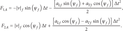
For this mode of movement, the plant noise covariance matrix (Q in (4)) models potential changes in longitudinal and transversal acceleration, the projection of those changes in velocity and heading, and independent drifts in the measurement biases, leading to the following definition:

$$\begin{array}{cc}& Q=F\left(\begin{array}{ccccccccc}\mathrm{0}& \mathrm{0}& \mathrm{0}& \mathrm{0}& \mathrm{0}& \mathrm{0}& \mathrm{0}& \mathrm{0}& \mathrm{0}\\ \mathrm{0}& \mathrm{0}& \mathrm{0}& \mathrm{0}& \mathrm{0}& \mathrm{0}& \mathrm{0}& \mathrm{0}& \mathrm{0}\\ \mathrm{0}& \mathrm{0}& \mathrm{0}& \mathrm{0}& \mathrm{0}& \mathrm{0}& \mathrm{0}& \mathrm{0}& \mathrm{0}\\ \mathrm{0}& \mathrm{0}& \mathrm{0}& \mathrm{0}& \mathrm{0}& \mathrm{0}& \mathrm{0}& \mathrm{0}& \mathrm{0}\\ \mathrm{0}& \mathrm{0}& \mathrm{0}& \mathrm{0}& {\sigma }_{a_L}^{\mathrm{2}}& \mathrm{0}& \mathrm{0}& \mathrm{0}& \mathrm{0}\\ \mathrm{0}& \mathrm{0}& \mathrm{0}& \mathrm{0}& \mathrm{0}& {\sigma }_{a_T}^{\mathrm{2}}& \mathrm{0}& \mathrm{0}& \mathrm{0}\\ \mathrm{0}& \mathrm{0}& \mathrm{0}& \mathrm{0}& \mathrm{0}& \mathrm{0}& {\sigma }_{\Delta \psi }^{\mathrm{2}}& \mathrm{0}& \mathrm{0}\\ \mathrm{0}& \mathrm{0}& \mathrm{0}& \mathrm{0}& \mathrm{0}& \mathrm{0}& \mathrm{0}& {\sigma }_{\Delta a_{Lm}}^{\mathrm{2}}& \mathrm{0}\\ \mathrm{0}& \mathrm{0}& \mathrm{0}& \mathrm{0}& \mathrm{0}& \mathrm{0}& \mathrm{0}& \mathrm{0}& {\sigma }_{\Delta a_{Tm}}^2\end{array}\right)F^T,\end{array}$$

(10)

where the nonzero values of the central matrix are parameters tuning the EKF behavior. They model the different errors and variables changes with time: ${\sigma }_{a_L}^2$ is the assumed longitudinal acceleration variance, ${\sigma }_{a_T}^2$ the assumed transversal acceleration variance, ${\sigma }_{\Delta \psi }^{\mathrm{2}}$ the assumed heading bias change variance, ${\sigma }_{\Delta a_{Lm}}^2$ the assumed longitudinal acceleration bias drift variance, and ${\sigma }_{\Delta a_{Tm}}^2$ the assumed transversal acceleration bias drift variance.

In order to reduce the errors of the acceleration signal, ZVU strategy is introduced. For this reason, a new prediction model must be taken into consideration whenever the foot is assumed to be on the floor. This is detected according to the procedure to be described in Section 4.3.1. If the foot does not move, the following assumptions can be made with respect to the state vector: the position is constant, the heading remains constant, and the acceleration and velocity related components are thus zero (and constant). Hence the prediction model relation in (7) may be simplified to

$$\begin{array}{cc}& \left(\begin{array}{c}{x}_P\\ y_p\\ {\left|v\right|}_p\\ {\psi }_p\\ a_{Lp}\\ a_{Tp}\\ {\Delta \psi }_p\\ {\Delta a}_{Lp}\\ {\Delta a}_{Tp}\end{array}\right)={\overrightarrow{x}}_p=f\left({\overrightarrow{x}}_f\right)=\left(\begin{array}{c}{x}_f\\ y_f\\ {\left|v\right|}_f\\ {\psi }_f\\ a_{Lf}\\ a_{Tf}\\ {\Delta \psi }_f\\ \Delta a_{Lf}\\ \Delta a_{Tf}\end{array}\right).\end{array}$$

(11)

Therefore, the prediction state relation is linear and we can simplify in this case the calculation of the Jacobian to the identity matrix:

$$\begin{array}{cc}& F=I.\end{array}$$

(12)

For the plant noise covariance matrix (Q in (4)), the same idea may be applied, which in this case consists in assigning zero variances (the values of the dynamic states are invariant) except for the cases of the offsets of the measurements that are nonzero.

It results in the following definition of this matrix:

$$\begin{array}{cc}& Q=\left(\begin{array}{ccccccccc}0& 0& 0& 0& 0& 0& 0& 0& 0\\ 0& 0& 0& 0& 0& 0& 0& 0& 0\\ 0& 0& 0& 0& 0& 0& 0& 0& 0\\ 0& 0& 0& 0& 0& 0& 0& 0& 0\\ 0& 0& 0& 0& 0& 0& 0& 0& 0\\ 0& 0& 0& 0& 0& 0& 0& 0& 0\\ 0& 0& 0& 0& 0& 0& {\sigma }_{\Delta \psi }^2& 0& 0\\ 0& 0& 0& 0& 0& 0& 0& {\sigma }_{\Delta a_{Lm}}^2& 0\\ 0& 0& 0& 0& 0& 0& 0& 0& {\sigma }_{\Delta a_{Tm}}^2\end{array}\right).\end{array}$$

(13)

As previously said, we have noticed that $\Delta \psi$ tends to change along time at different rates quite slowly when the pedestrian follows constant heading paths or stops and much faster along pedestrians turns. This is addressed in this filter by changing the plant noise covariance matrix for ZVU for both heading and heading bias. In order to do so, turns are detected by differentiating ZVU heading measurements from consecutive stances and comparing the difference against a constant threshold of 10 degrees. If a turn is detected, the plant noise covariance is changed to the one described in (14). Consider

$$\begin{array}{cc}& Q=\left(\begin{array}{ccccccccc}0& 0& 0& 0& 0& 0& 0& 0& 0\\ 0& 0& 0& 0& 0& 0& 0& 0& 0\\ 0& 0& 0& 0& 0& 0& 0& 0& 0\\ 0& 0& 0& {\sigma }_{\delta \psi }^2& 0& 0& 0& 0& 0\\ 0& 0& 0& 0& 0& 0& 0& 0& 0\\ 0& 0& 0& 0& 0& 0& 0& 0& 0\\ 0& 0& 0& 0& 0& 0& {\sigma }_{\Delta \psi }^2+{\sigma }_{\delta \psi }^2& 0& 0\\ 0& 0& 0& 0& 0& 0& 0& {\sigma }_{\Delta a_{Lm}}^2& 0\\ 0& 0& 0& 0& 0& 0& 0& 0& {\sigma }_{\Delta a_{Tm}}^2\end{array}\right),\end{array}$$

(14)

where ${\sigma }_{\delta \psi }^2$ is an additional covariance for both heading and heading bias drift.

Equation (7) has a problem for low velocities, which is the instability due to the division in the heading prediction (fourth component). To eliminate this problem it is assumed that very slow foot movement is not compatible with turns. For this reason, a prediction model in which zero (constant) transverse acceleration is taken into consideration is applied when ${\left|v\right|}_f$ is small. This model changes (7) to

$$\begin{array}{l}\left(\begin{array}{l}{x}_P\\ y_p\\ {\left|v\right|}_p\\ {\psi }_p\\ a_{Lp}\\ a_{Tp}\\ {\Delta \psi }_p\\ {\Delta a}_{Lp}\\ {\Delta a}_{Tp}\end{array}\right)\\ \hspace{1em}={\overrightarrow{x}}_p=f\left({\overrightarrow{x}}_f\right)\\ \hspace{1em}=\left(\begin{array}{l}{x}_f+{\left|v\right|}_f\cos \left({\psi }_f\right)\Delta t+\frac{a_{Lf}\cos \left({\psi }_f\right){\Delta t}^2}{2}\\ y_f+{\left|v\right|}_f\sin \left({\psi }_f\right)\Delta t+\frac{a_{Lf}\sin \left({\psi }_f\right){\Delta t}^2}{2}\\ {\left|v\right|}_f+a_{Lf}\Delta t\\ {\psi }_f\\ a_{Lf}\\ a_{Tf}\\ \Delta {\psi }_f\\ \Delta a_{Lf}\\ \Delta a_{Tf}\end{array}\right).\end{array}$$

(15)

The associated Jacobian for this case would be

$$\begin{array}{cc}& F=\left(\begin{array}{ccccccccc}1& 0& \cos \left({\psi }_f\right)\Delta t& -\left({\left|v\right|}_f\Delta t+\frac{{\Delta t}^2}{2}{a}_{Lf}\right)\sin \left({\psi }_f\right)& \frac{{\Delta t}^2}{2}\cos \left({\psi }_f\right)& 0& 0& 0& 0\\ 0& 1& \sin \left({\psi }_f\right)\Delta t& \left({\left|v\right|}_f\Delta t+\frac{{\Delta t}^2}{2}{a}_{Lf}\right)\cos \left({\psi }_f\right)& \frac{{\Delta t}^2}{2}\sin \left({\psi }_f\right)& 0& 0& 0& 0\\ 0& 0& 1& 0& \Delta t& 0& 0& 0& 0\\ 0& 0& 0& 1& 0& 0& 0& 0& 0\\ 0& 0& 0& 0& 1& 0& 0& 0& 0\\ 0& 0& 0& 0& 0& 1& 0& 0& 0\\ 0& 0& 0& 0& 0& 0& 1& 0& 0\\ 0& 0& 0& 0& 0& 0& 0& 1& 0\\ 0& 0& 0& 0& 0& 0& 0& 0& 1\end{array}\right).\end{array}$$

(16)

Finally, for this case we use the following definition of plant noise covariance (Q in (4)), equivalent to the one in (10), with F as described in (16):

$$\begin{array}{cc}& Q=F\left(\begin{array}{ccccccccc}\mathrm{0}& \mathrm{0}& \mathrm{0}& \mathrm{0}& \mathrm{0}& \mathrm{0}& \mathrm{0}& \mathrm{0}& \mathrm{0}\\ \mathrm{0}& \mathrm{0}& \mathrm{0}& \mathrm{0}& \mathrm{0}& \mathrm{0}& \mathrm{0}& \mathrm{0}& \mathrm{0}\\ \mathrm{0}& \mathrm{0}& \mathrm{0}& \mathrm{0}& \mathrm{0}& \mathrm{0}& \mathrm{0}& \mathrm{0}& \mathrm{0}\\ \mathrm{0}& \mathrm{0}& \mathrm{0}& \mathrm{0}& \mathrm{0}& \mathrm{0}& \mathrm{0}& \mathrm{0}& \mathrm{0}\\ \mathrm{0}& \mathrm{0}& \mathrm{0}& \mathrm{0}& {\sigma }_{a_L}^{\mathrm{2}}& \mathrm{0}& \mathrm{0}& \mathrm{0}& \mathrm{0}\\ \mathrm{0}& \mathrm{0}& \mathrm{0}& \mathrm{0}& \mathrm{0}& {\sigma }_{a_T}^{\mathrm{2}}& \mathrm{0}& \mathrm{0}& \mathrm{0}\\ \mathrm{0}& \mathrm{0}& \mathrm{0}& \mathrm{0}& \mathrm{0}& \mathrm{0}& {\sigma }_{\Delta \psi }^{\mathrm{2}}& \mathrm{0}& \mathrm{0}\\ \mathrm{0}& \mathrm{0}& \mathrm{0}& \mathrm{0}& \mathrm{0}& \mathrm{0}& \mathrm{0}& {\sigma }_{\Delta a_{Lm}}^{\mathrm{2}}& \mathrm{0}\\ \mathrm{0}& \mathrm{0}& \mathrm{0}& \mathrm{0}& \mathrm{0}& \mathrm{0}& \mathrm{0}& \mathrm{0}& {\sigma }_{\Delta a_{Tm}}^{\mathrm{2}}\end{array}\right)F^T.\end{array}$$

(17)

In addition, protection of the predicted and filtered states is carried out: if the magnitude of the filtered or predicted velocity ( ${\left|v\right|}_f$ or ${\left|v\right|}_p$ ) is negative, it is changed to zero.

4.1.2. Measurement Model

This filter processes the accelerometer and heading measurements provided by the IMU and position measurements (from GPS or from an indoor localization system). When several measurements arrive at the same time, they are processed successively without prediction phases. Whenever a new measurement is received, it must be checked whether the time instant corresponds to ZVU, using the procedure described in Section 4.3.1. Next we will detail the filtering associated equations for each type of measurement, for the cases with or without ZVU.

First let us consider the position measurement processing, compatible for both with and without ZVU situations. The position measurements vector ( ${\overrightarrow{x}}_m$ ) is a 2D vector containing the X and Y coordinates of the position measured in the inertial coordinate system at a specific time. Equation (18) defines the components in (5), necessary to complete the filtering phase for position measurements. Consider

$$\begin{array}{cc}& {\overrightarrow{x}}_m=\left(\begin{array}{c}{x}_m\\ y_m\end{array}\right);\hspace{1em}\hspace{1em}h\left({\overrightarrow{x}}_p\right)=h\left(\left(\begin{array}{c}{x}_P\\ y_p\\ {\left|v\right|}_p\\ {\psi }_p\\ a_{Lp}\\ a_{Tp}\\ {\Delta \psi }_p\\ {\Delta a}_{Lp}\\ {\Delta a}_{Tp}\end{array}\right)\right)=\left(\begin{array}{c}{x}_p\\ y_p\end{array}\right),\\ H=\left(\begin{array}{ccccccccc}\mathrm{1}& \mathrm{0}& \mathrm{0}& \mathrm{0}& \mathrm{0}& \mathrm{0}& \mathrm{0}& \mathrm{0}& \mathrm{0}\\ \mathrm{0}& \mathrm{1}& \mathrm{0}& \mathrm{0}& \mathrm{0}& \mathrm{0}& \mathrm{0}& \mathrm{0}& \mathrm{0}\end{array}\right),\\ R=\left(\begin{array}{cc}{\sigma }_P^{\mathrm{2}}& \mathrm{0}\\ \mathrm{0}& {\sigma }_P^{\mathrm{2}}\end{array}\right),\end{array}$$

(18)

where ${\sigma }_P^2$ is the assumed variance of the error of the positioning system.

The case of the acceleration is more complex, as we must distinguish the cases with and without ZVU. In the cases without ZVU, the measurements of the acceleration ( $a_{Lm}$ and $a_{Tm}$ ) are the projection of the acceleration values, initially in foot reference frame, on the horizontal plane (body frame). Equation (19) specifies the terms needed to complete the filtering according to (5). The model considers the effect of the acceleration bias on the acceleration measures. Consider

$$\begin{array}{cc}& {\overrightarrow{x}}_m=\left(\begin{array}{c}{a}_{Lm}\\ a_{Tm}\end{array}\right);\hspace{1em}\hspace{1em}h\left({\overrightarrow{x}}_p\right)=\left(\begin{array}{c}{a}_{Lp}+{\Delta a}_{Lp}\\ a_{Tp}+{\Delta a}_{Tp}\end{array}\right),\\ H=\left(\begin{array}{ccccccccc}0& 0& 0& 0& 1& 0& 0& 1& 0\\ 0& 0& 0& 0& 0& 1& 0& 0& 1\end{array}\right),\\ R=\left(\begin{array}{cc}{\sigma }_A^2& 0\\ 0& {\sigma }_A^2\end{array}\right),\end{array}$$

(19)

where ${\sigma }_A^2$ is the assumed variance of the error of the acceleration measurements of the IMU sensors.

The measurement model changes whenever it is detected that the foot is resting on the ground (i.e., it is ZVU instant). In that case, if we are on a flat surface, the acceleration should be zero, which means that if the value of the projected horizontal measurement is different from zero, it is due to the bias of the sensor. In addition, zero velocity magnitude and acceleration pseudo-measurements are introduced in the measurement vector and model. This forces the filter velocity and acceleration states to become almost zero and makes the position almost constant during this time interval, while calibrating the bias terms. The variances of those pseudo-measurements are nearly 0 to reaffirm the accuracy of their values. This results in the following measurement equations for this case:

$$\begin{array}{cc}& {\overrightarrow{x}}_m=\left(\begin{array}{c}0\\ 0\\ 0\\ a_{Lm}\\ a_{Tm}\end{array}\right);\hspace{1em}\hspace{1em}h\left({\overrightarrow{x}}_p\right)=\left(\begin{array}{c}{\left|v\right|}_p\\ a_{Lp}\\ a_{Tp}\\ {\Delta a}_{Lp}\\ {\Delta a}_{Tp}\end{array}\right)\\ H=\left(\begin{array}{ccccccccc}0& 0& 1& 0& 0& 0& 0& 0& 0\\ 0& 0& 0& 0& 1& 0& 0& 0& 0\\ 0& 0& 0& 0& 0& 1& 0& 0& 0\\ 0& 0& 0& 0& 0& 0& 0& 1& 0\\ 0& 0& 0& 0& 0& 0& 0& 0& 1\end{array}\right)\\ R=\left(\begin{array}{ccccc}{\sigma }_{{\left|v\right|}_{pm}}^2& 0& 0& 0& 0\\ 0& {\sigma }_{A_{pm}}^2& 0& 0& 0\\ 0& 0& {\sigma }_{A_{pm}}^2& 0& 0\\ 0& 0& 0& {\sigma }_A^2& 0\\ 0& 0& 0& 0& {\sigma }_A^2\end{array}\right),\end{array}$$

(20)

where ${\sigma }_{{\left|v\right|}_{pm}}^2$ is the variance of the error of the velocity pseudo-measurements and ${\sigma }_{A_{pm}}^2$ is the assumed variance of the error of the acceleration pseudo-measurements. Both should be very low values but not making the filter unstable.

Finally, the processing of heading measurements ( ${\psi }_m$ ) is independent of the state of the foot, not changing in time. The heading angle provided by the IMU sensor is introduced into the Kalman filter as described in (21). The associated model takes into consideration the presence of bias in this measurement. ${\sigma }_{\psi }^2$ is the assumed variance of the heading measurements. Consider

$$\begin{array}{cc}& {\overrightarrow{x}}_m=\left({\psi }_m\right);\hspace{1em}\hspace{1em}h\left({\overrightarrow{x}}_p\right)=\left({\psi }_p+\Delta {\psi }_p\right),\\ H=\left(\begin{array}{ccccccccc}0& 0& 0& 1& 0& 0& 1& 0& 0\end{array}\right),\\ R=\left({\sigma }_{\psi }^2\right).\end{array}$$

(21)

4.2. Complementary KF

The second proposed filter is a complementary Kalman filter, which will process three different kinds of measurements:

• (i)

  position: ( $x_m$ , $y_m$ );

• (ii)

  acceleration: ( $a_{Lm}$ , $a_{Tm}$ );

• (iii)

  heading: ${\psi }_m$ .

The basic idea behind this solution is the aiding of a simplified INS integration process by estimating and correcting the accumulated bias from the offsets between the position sensor measures and the current integrated INS based trajectory. In order to introduce this type of filter, let us assume that: $(1)$ there are no position measures and $(2)$ heading and acceleration measures have no error. For short time intervals and for walking pedestrians, we could integrate the trajectory using the IMU measures as follows in (22), where the left part of each assignment refers to current time inertial estimates of x, y, velocity magnitude, and heading ( $x_I$ , $y_I$ , ${\left|v\right|}_I$ , and ${\psi }_I$ ). The right parts of the assignments contain current time IMU measures ( $a_{Lm}$ , $a_{Tm}$ , projected into body frame, and ${\psi }_m$ ) and previous time inertial estimates of x, y, and velocity magnitude ( $x_I$ , $y_I$ , and ${\left|v\right|}_I$ ). Consider

$$\begin{array}{l}{x}_I=x_I+{\left|v\right|}_I\cos \left({\psi }_I\right)\Delta t\\ \hspace{1em}\hspace{1em}+\left[a_{Lm}\cos \left({\psi }_I\right)-a_{Tm}\sin \left({\psi }_I\right)\right]\frac{{\Delta t}^{\mathrm{2}}}{\mathrm{2}},\\ y_I=y_I+{\left|v\right|}_I\sin \left({\psi }_I\right)\Delta t\\ \hspace{1em}\hspace{1em}+\left[a_{Lm}\sin \left({\psi }_I\right)+a_{Tm}\cos \left({\psi }_I\right)\right]\frac{{\Delta t}^{\mathrm{2}}}{\mathrm{2}},\\ \hspace{1em}\hspace{1em}\hspace{1em}\hspace{1em}{\left|v\right|}_I={\left|v\right|}_I+a_{Lm}\Delta t,\\ \hspace{1em}\hspace{1em}\hspace{1em}\hspace{1em}\hspace{1em}\hspace{1em}{\psi }_I={\psi }_m.\end{array}$$

(22)

This kind of processing would be accurate in the following conditions: $(1)$ measurements without bias; $(2)$ negligible transversal-to-foot movement; and $(3)$ reduced effect of the pitching movement of the foot. A classical alternative approach to the centralized smoothing consists in performing an estimation of the bias in parallel with the inertial integration and removing the estimated bias values along the processing. The state vector of the filter contains the errors of position and velocity and the bias of the measurements, described in the next equation for the filtered estimation (for the predicted estimation, just change the f subindex to p):

$$\begin{array}{cc}& {\overrightarrow{x}}_f={\left[\begin{array}{cccccc}\Delta x_f& \Delta y_f& \Delta {\left|v\right|}_f& \Delta {\psi }_f& \Delta a_{Lf}& \Delta a_{Tf}\end{array}\right]}^T.\end{array}$$

(23)

The proposed implementation of a complementary filter for our model will be formed of the following steps.

• (1)

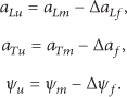
  Subtract the previously estimated bias (from previous measures) from the acceleration and heading measurements, defining unbiased measures to be described using subindex u:

  $$\begin{array}{cc}& a_{Lu}=a_{Lm}-\Delta a_{Lf},\\ a_{Tu}=a_{Tm}-\Delta a_f,\\ {\psi }_u={\psi }_m-\Delta {\psi }_f.\end{array}$$

  (24)

• (2)

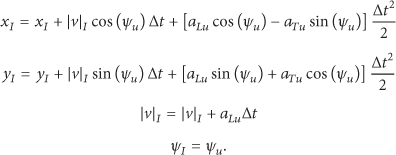
  Update the inertial state estimates using a slightly modified version of (22), with the bias corrected measures:

  $$\begin{array}{cc}& x_I=x_I+{\left|v\right|}_I\cos \left({\psi }_u\right)\Delta t+\left[a_{Lu}\cos \left({\psi }_u\right)-a_{Tu}\sin \left({\psi }_u\right)\right]\frac{{\Delta t}^{\mathrm{2}}}{2}\\ y_I=y_I+{\left|v\right|}_I\sin \left({\psi }_u\right)\Delta t+\left[a_{Lu}\sin \left({\psi }_u\right)+a_{Tu}\cos \left({\psi }_u\right)\right]\frac{{\Delta t}^{\mathrm{2}}}{2}\\ {\left|v\right|}_I={\left|v\right|}_I+a_{Lu}\Delta t\\ {\psi }_I={\psi }_u.\end{array}$$

  (25)

• (3)

  Perform the prediction and filtering processes described in Sections 4.2.1 and 4.2.2 in order to update the filtered bias state values.

• (4)

  Correct the errors due to the integration process, to obtain the output of the complete processing:

  $$\begin{array}{cc}& x_u=x_I-\Delta x_f,\\ y_u=y_I-\Delta y_f,\\ {\left|v\right|}_u={\left|v\right|}_I-\Delta {\left|v\right|}_f.\end{array}$$

  (26)

• (5)

  The filter is based on linearization of the error equations in (25), to be described in Section 4.2.2. Finally, to reduce the effect of the bias in this linearization, the filter turns the position integration drift estimates into zero by correcting them in the inertial position and velocity estimates. Consider

  $$\begin{array}{cc}& x_I=x_u;\hspace{1em}\hspace{1em}{y}_I=y_u\\ \Delta x_f=\mathrm{0};\hspace{1em}\hspace{1em}\Delta y_f=\mathrm{0}.\end{array}$$

  (27)

• (6)

  For velocity bias, this is done if the measurement is not related to ZVU instant. Consider

  $$\begin{array}{cc}& {\left|v\right|}_I={\left|v\right|}_u;\hspace{1em}\hspace{1em}\Delta {\left|v\right|}_f=\mathrm{0}.\end{array}$$

  (28)

• (7)

  Meanwhile, if we are in ZVU instant according to the detectors described in Section 4.3.1, the inertial integrated velocity is converted into zero:

  $$\begin{array}{cc}& \Delta {\left|v\right|}_f={\left|v\right|}_I+\Delta {\left|v\right|}_f;\hspace{1em}\hspace{1em}{\left|v\right|}_I=\mathrm{0}.\end{array}$$

  (29)

  The unbiased output of the complete processing would be the vector:

  $$\begin{array}{cc}& {\overrightarrow{x}}_I={\left[\begin{array}{cccc}{x}_I& y_I& {\left|v\right|}_I& {\psi }_I\end{array}\right]}^T.\end{array}$$

  (30)

So, in order to complete the description, we must describe the complementary KF prediction and measurement models and algorithms (step $(3)$ of previous algorithm). This filter does not process the raw input position and acceleration measurements. Instead, it processes modified measurements, which are independent of pedestrian dynamics, and just containing bias related terms. In next subsections we will describe both the prediction and measurement processing approaches for the complementary KF. The complete processing scheme is depicted in Figure 3.

Figure 3

Complementary KF complete processing architecture.

4.2.1. Prediction Model

The Kalman filter needs to estimate the described offset/bias parameters. The bias parameters remain mainly constant, but the kinematic estimation offsets tend to accumulate due to the INS integration process. So, the prediction model includes terms related to this propagation, resulting in a linear relation between previous filtered estimation and current time predicted estimation, where the state propagation matrix (F) results from analyzing the influence that a small error in the magnitude of the filtered estimate and in the new measurements can have on the estimated position and velocity using the integration equations in (25):

$$\begin{array}{cc}& F=\left(\begin{array}{cccccc}1& 0& \cos \left({\psi }_u\right)\Delta t& F_{\mathrm{1,4}}& \frac{\cos \left({\psi }_u\right){\Delta t}^2}{2}& \frac{-\sin \left({\psi }_u\right){\Delta t}^2}{2}\\ 0& 1& \sin \left({\psi }_u\right)\Delta t& F_{\mathrm{2,4}}& \frac{\sin \left({\psi }_u\right){\Delta t}^2}{2}& \frac{{\cos \left({\psi }_u\right)\Delta t}^2}{2}\\ 0& 0& 1& 0& \Delta t& 0\\ 0& 0& 0& 1& 0& 0\\ 0& 0& 0& 0& 1& 0\\ 0& 0& 0& 0& 0& 1\end{array}\right),\end{array}$$

(31)

where

$$\begin{array}{cc}& F_{\mathrm{1,4}}=-\left({\left|v\right|}_I\Delta t+a_{Lu}\frac{{\Delta t}^2}{2}\right)\sin \left({\psi }_u\right)-a_{Tu}\frac{{\Delta t}^2}{2}\cos \left({\psi }_u\right),\\ F_{\mathrm{2,4}}=\left({\left|v\right|}_I\Delta t+a_{Lu}\frac{{\Delta t}^2}{2}\right)\cos \left({\psi }_u\right)-a_{Tu}\frac{{\Delta t}^2}{2}\sin \left({\psi }_u\right).\end{array}$$

(32)

Regarding the definition of the prediction of the state in the EKF equations in (4), we have

$$\begin{array}{cc}& \left(\begin{array}{c}\Delta x_p\\ \Delta y_p\\ \Delta {\left|v\right|}_p\\ \Delta {\psi }_p\\ \Delta a_{Lp}\\ \Delta a_{Tp}\end{array}\right)={\overrightarrow{x}}_p=f\left({\overrightarrow{x}}_f\right)=F{\overrightarrow{x}}_f=F\left(\begin{array}{c}\Delta x_f\\ \Delta y_f\\ \Delta {\left|v\right|}_f\\ \Delta {\psi }_f\\ \Delta a_{Lf}\\ \Delta a_{Tf}\end{array}\right).\end{array}$$

(33)

The associated Jacobian of the transformation is F, directly, and the covariance matrix of the plant noise (Q in (4)) in this case can be modeled as follows:

$$\begin{array}{cc}& Q=F{Q}_0{F}^T=F\left(\begin{array}{cccccc}0& 0& 0& 0& 0& 0\\ 0& 0& 0& 0& 0& 0\\ 0& 0& 0& 0& 0& 0\\ 0& 0& 0& {\sigma }_{\Delta \psi }^2& 0& 0\\ 0& 0& 0& 0& {\sigma }_{\Delta a_{Lm}}^2& 0\\ 0& 0& 0& 0& 0& {\sigma }_{\Delta a_{Tm}}^2\end{array}\right)F^T.\end{array}$$

(34)

Again the speed of change of $\Delta \psi$ along turns is addressed by changing the plant noise covariance matrix for ZVU for heading bias. In the case a turn is detected (using the same method described in Section 4.1.1) the plant noise covariance is changed as described in (35). Consider

$$\begin{array}{cc}& Q=F{Q}_0{F}^T=F\left(\begin{array}{cccccc}0& 0& 0& 0& 0& 0\\ 0& 0& 0& 0& 0& 0\\ 0& 0& 0& 0& 0& 0\\ 0& 0& 0& {{\sigma }_{\delta \psi }^2+\sigma }_{\Delta \psi }^2& 0& 0\\ 0& 0& 0& 0& {\sigma }_{\Delta a_{Lm}}^2& 0\\ 0& 0& 0& 0& 0& {\sigma }_{\Delta a_{Tm}}^2\end{array}\right)F^T.\end{array}$$

(35)

4.2.2. Measurement Model

The measurements that are considered in the filtering process should enable the estimation of the integration and measurement offsets. This means that they are either preprocessed versions of the input measurements removing the pedestrian kinematics or measurements taken during time intervals where some of the kinematic variables are known. For instance, when the foot is placed on the floor (ZVU), the values of the acceleration, velocity and angular rate are zero and the position and the heading is constant.

Next we will detail the processing associated to each kind of input measurements, following the notation in (5). First we will explain the position measurement processing, for the cases with and without ZVU. The unbiased position measurements vector ( ${\overrightarrow{x}}_m$ ) is a 2D vector containing the X and Y coordinates of the position of the individual measured in the inertial coordinate system at a specific time. From this measure, we derive an observation of the inertial position error terms in X and Y coordinates by subtracting the integrated inertial position. This integrated inertial position contains the accumulated drift ( $\Delta x_p,\Delta y_p$ ). The subtraction removes the dependency with pedestrian position, resulting in the measurement model equation (36). Consider

$$\begin{array}{cc}& {\overrightarrow{x}}_m=\left(\begin{array}{c}{x}_m-x_I\\ y_m-y_I\end{array}\right);\\ h\left({\overrightarrow{x}}_p\right)=h\left(\left(\begin{array}{c}\Delta x_p\\ \Delta y_p\\ \Delta {\left|v\right|}_p\\ \Delta {\psi }_p\\ \Delta a_{Lp}\\ \Delta a_{Tp}\end{array}\right)\right)=\left(\begin{array}{c}{-\Delta x}_p\\ -\Delta y_p\end{array}\right),\\ H=\left(\begin{array}{cccccc}-\mathrm{1}& \mathrm{0}& \mathrm{0}& \mathrm{0}& \mathrm{0}& \mathrm{0}\\ \mathrm{0}& -\mathrm{1}& \mathrm{0}& \mathrm{0}& \mathrm{0}& \mathrm{0}\end{array}\right),\\ R=\left(\begin{array}{cc}{\sigma }_P^{\mathrm{2}}& \mathrm{0}\\ \mathrm{0}& {\sigma }_P^{\mathrm{2}}\end{array}\right),\end{array}$$

(36)

where ${\sigma }_P^2$ is again the assumed variance of the error of the positioning system.

Acceleration measurements are just processed in the time intervals where the foot is on the ground (ZVU). In that case, if the value of the measurement is different from zero, it is due to the bias of the sensor. This results into the following measurement equations for this case:

$$\begin{array}{cc}& {\overrightarrow{x}}_m=\left(\begin{array}{c}{a}_{Lm}\\ a_{Tm}\end{array}\right);\hspace{1em}\hspace{1em}h\left({\overrightarrow{x}}_p\right)=\left(\begin{array}{c}{\Delta a}_{Lp}\\ {\Delta a}_{Tp}\end{array}\right),\\ H=\left(\begin{array}{cccccc}0& 0& 0& 0& 1& 0\\ 0& 0& 0& 0& 0& 1\end{array}\right),\\ R=\left(\begin{array}{cc}{\sigma }_A^2& 0\\ 0& {\sigma }_A^2\end{array}\right).\end{array}$$

(37)

Finally, we can also introduce velocity pseudo-measurements during ZVU intervals. During this phase, if there is some nonzero velocity according to the inertial integration, it will be due to the presence of drift in the integration process (nonzero $\Delta \left|v\right|$ ). So, the value of the inertial estimation of velocity is taken as the pseudo-measurement, resulting in the next equation:

$$\begin{array}{cc}& {\overrightarrow{x}}_m=\left({\left|v\right|}_I\right);\hspace{1em}\hspace{1em}h\left({\overrightarrow{x}}_p\right)=\left(\Delta {\left|v\right|}_p\right),\\ H=\left(\begin{array}{cccccc}\mathrm{0}& \mathrm{0}& \mathrm{1}& \mathrm{0}& \mathrm{0}& \mathrm{0}\end{array}\right),\\ R=\left({\sigma }_{\Delta \left|v\right|pm}^2\right).\end{array}$$

(38)

Here, ${\sigma }_{\Delta \left|v\right|pm}^2$ would be an assumed variance for the pseudo-measurement, very small but not making the filter unstable.

4.3. Support Algorithms for Previous Filters

Next we will detail some of the supporting algorithms that can be used for the different localization architectures: the process for ZVU detection and the processes enabling the calculation of position measurements in indoor deployment, based on RSS measurements from distributed sensors network.

4.3.1. Zero Velocity Update Instants Detection

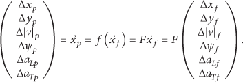
As it is common in this kind of systems, ZVU have been included in this work to reduce the errors of the inertial sensors. The chosen algorithms, to detect in which instants the foot is placed on the ground, are the acceleration moving variance detector (MV) and angular rate energy detector (ARE). They are defined in (39), where W is the number of samples in a window, $a_k$ the acceleration measures, ${\stackrel{-}{a}}_W$ and ${\sigma }_a^2$ the average and the variance of the acceleration values in that window, and ${\omega }_k$ the gyroscope samples [23]. There are two MV detectors, one for each acceleration component, longitudinal acceleration and transversal acceleration. Consider

$$\begin{array}{cc}& \text{MV}=\frac{1}{{\sigma }_a^{2}W}{\displaystyle \sum }_{k=n}^{n+W-1}{\parallel a_k-{\stackrel{-}{a}}_W\parallel }^2,\\ \text{ARE}=\frac{1}{{\sigma }_{\omega }^{2}W}{\displaystyle \sum }_{k=n}^{n+W-1}{\parallel {\omega }_k\parallel }^2.\end{array}$$

(39)

The first detector is based on the fact that the measured acceleration is approximately constant in the stance phase, whereas the second one is based on the lack of rotation of the foot during this phase (see Figure 2). The foot is decided to be in an instant of ZVU whenever both MV and ARE detectors decide that it is the case.

In our implementation, a window length contains 5 samples, which has been empirically found to be a suitable value for the characteristics of the IMU acceleration and rate of turn signals: remember one step takes about 1 second, the sampling frequency is 50 Hz, and the stance phase is about 40% of the step, so this phase lasts around 20 samples. The thresholds, initialized to fixed values (2.5 for MV, 1 for ARE), have been found empirically, although an adaptive threshold could be incorporated (for instance, based on a constant false alarm rate design). All the detector parameters were selected in order to minimize the possibility of detecting a nonzero velocity sample as a zero velocity sample, as this event is much more problematic than not detecting a few zero velocity samples, due to the potential corruption on bias estimations, potentially resulting in increased error in both EKF and complementary filter.

4.3.2. Position Estimation

All presented systems are loosely coupled, based on high update rate IMU measures and lower rate position updates. Those position updates may come either from GPS for outdoor localization/navigation applications or from indoor localization systems. Along time, the system will use the different available position measurements, tuning the appropriate measurement model equations ((18) and (36) for each of the described systems) to the quality of the sensor.

In the case of indoor localization, in our implementation, position estimations are calculated through a weighted circular multilateration algorithm that works on RSS measurements. The estimation of the distances between the user and the deployed beacon nodes is based on a lognormal channel model. The details of this algorithm are out of the scope of this paper; for further information refer to [24].

5. Result and Discussion

In this section we described the following: (a) the experimental deployment that has been used for the evaluation of the filters in indoor environments (Section 5.1), (b) the values of the filter parameters for both implementations (Section 5.2), (c) the accuracy assessment (Section 5.3), (d) the applicability of this system for outdoor pedestrian tracking (Section 5.4), and (e) the computational load associated with each of the filters (Section 5.5), including a comparative analysis with other methods in the literature.

5.1. Experimental Deployment

Two different scenarios have been considered to test the performance of the tracking solutions. In those scenarios, the individual that performs the tests is equipped with a pair of MTx IMUs from the company Xsens [21] which, as said before, gather the information measured by the inertial sensors as well as the magnetometer at a sampling rate of 50 Hz. Two sensors are placed on both feet of the individual. In addition, the individual carries an IRIS mote (from MEMSIC [25]) to enable continuous localization using a ZigBee RSS-based positioning system. This device communicates with the beacon nodes deployed in the environment using the IEEE 802.15.4 communication protocol.

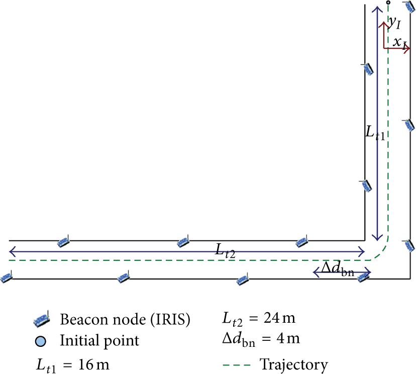
The first scenario is shown in Figures 4 and 5. It consists in a trajectory of about 40 meters along a corridor in which there is a turn of 90° after walking 16 meters. It also shows the deployment of the IRIS beacon nodes. The movement starts at the top right of the map in Figure 4.

Figure 4

Scenario 1 of trajectory and deployment.

Figure 5

Picture of experimental deployment.

To carry out RSS-based localization, 12 IRIS motes have been deployed on the walls of the corridor, in a very controlled way in order to be able to easily reproduce the experiment in similar environments. The distance between the motes is 4 meters and they are placed at a height of 2 meters to prevent signal shadowing due to objects. In addition, they have been placed alternatively on the walls to provide good signal coverage of a minimum of 3 nonaligned motes at every point of the trajectory. The mote obtains the RSS measurement every 100 ms. The parameters of the lognormal channel model necessary for the positioning algorithm have been estimated using methods derived from [26]. To estimate those parameters, measurements were taken in a grid of points, every 1.2 meters. The estimated channel parameters are $A=-84$  dB and $\eta =2.4$ . It should be noted that those parameters are specific for each deployment. Therefore, it is necessary to perform a calibration of the positioning system to obtain high accuracy performance.

Eight individuals have travelled this scenario. The time that the individuals needed to cover the distance varies between 30 and 40 seconds. This trajectory has been travelled 5 times for each individual with a sensor placed on each foot. So ten signals per user (5 walks with two IMUs, one per foot) were available to test the system, resulting in a total of 80 test trajectories.

The second scenario is the same as the first one, but in this case it is a closed loop trajectory, with a 180° turn at the end of the corridor to come back again and return to the initial point. In this way, the total longitude is around 80 meters, travelled on a time interval between 60 and 70 seconds.

5.2. Filter Parameters

Although in the derivation of the systems we have used a common notation for many of the filter parameters, the parameters were manually tuned for both of the filters independently, in order to attain a good compromise between smoothing and robustness. This tuning was performed on the basis of the measurements from two users in several scenarios different than those in the evaluation: $(1)$ movement along a corridor; $(2)$ turn in a corner; and $(3)$ circular movement (with 3 meters radius) in a wide room. The parameters of both filters are described in Table 1, where N/A means the parameter is not applicable to this kind of filter. Please note that the most adequate values of most parameters would be dependent on the actual deployed sensors, and a fine-tuning would be necessary for other sensor quality levels.

Table 1

Filter parameters.

Parameter	Centralized EKF values	Complementary KF value
${\sigma }_{{\mathrm{a}}_L}$	30 m/s2	N/A
${\sigma }_{{\mathrm{a}}_T}$	15 m/s2	N/A
${\sigma }_{\mathrm{\Delta }\mathrm{\psi }}$	10−7 rad	10−5 rad
${\sigma }_{\mathrm{\delta }\mathrm{\psi }}$	0.01 rad	0.01 rad
${\sigma }_{{\mathrm{\Delta }\mathrm{a}}_{Lm}}$	10−4 m/s2	10−4 m/s2
${\sigma }_{{\mathrm{\Delta }\mathrm{a}}_{Tm}}$	10−4 m/s2	10−4 m/s2
${\sigma }_{\mathrm{P}}$	0.5 m	2.0 m
${\sigma }_{\mathrm{A}}$	0.2 m/s2	0.2 m/s2
${\sigma }_{\mathrm{\psi }}$	0.005 rad	N/A
${\sigma }_{{\left|v\right|}_{pm}}$	10−8 m/s	N/A
${\sigma }_{A_{pm}}$	10−8 m/s	N/A
${\sigma }_{A\left|v\right|pm}$	N/A	1 m/s

The described parameters show that the centralized EKF has a limited capability to smooth acceleration measurements. This permits thinking on a third potential solution based on a EKF filter which, instead of processing acceleration as measurements, will use them as control inputs (with acceleration biases calculated along ZVU intervals and removed before applying control inputs in prediction), with reduced state vector and therefore reduced computational cost. The associated accuracy would be quite similar to that of the centralized EKF.

5.3. Comparative Accuracy Evaluation

This section gathers the results achieved using the proposed filters, together with other results to be used as a comparison benchmark, as the ones achieved using double integration of the acceleration or stand-alone RSS positioning.

Figure 6 shows an example of the positional data received along one user trip in scenario 2. Here we have both RSS derived positions and the INS integrated position, provided that no bias is estimated or corrected. The INS double integration of the measurements does not contain a way to counteract it, so it is expected that the errors continue growing as long as the experiments last. INS integration has ZVU correction to reduce the drift speed due to the double integration of erroneous acceleration measurements.

Figure 6

Example position (RSS measures) and INS integrated trajectory.

In Figures 7 and 8 the results of processing the previous measures with each of the proposed filters are depicted. In those figures, it is very clear that once the heading is estimated, both filters are capable of tracking the movement.

Figure 7

Centralized EKF execution.

Figure 8

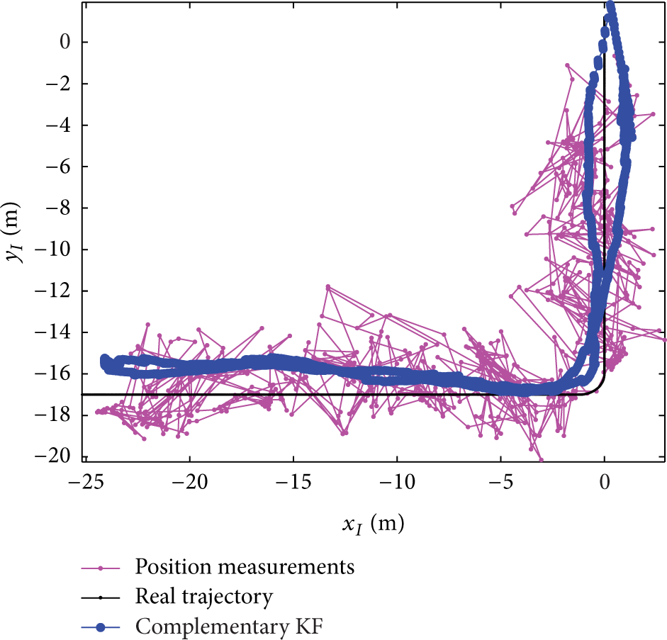
Complementary KF execution.

Figure 9 shows how the 3D complementary filter by Foxlin [15] performs in the same scenario.

Figure 9

Foxlin [15] 3D complementary KF execution.

In order to measure the performance of the different trackers, the error considered for comparison is the Euclidean distance between the estimated point and the approximated real position of the individual at that instant, using a linear movement model along the center of the corridors. This model assumes constant velocity between turns (the users maintained quasi-constant speed in each corridor), but of course, as perfectly smooth movement is not possible, there will always be a residual error due to this interpolation, in the order of 20–40 cm (related to maximum longitudinal excursion of half of a step, and less than 0.5 meter lateral offset). This additive error component is smaller than the error we are measuring, as it will be shown in the following tables of results. This way, the average and the standard deviation of the error along a trajectory can be estimated. Five values are provided for each scenario:

• (a)

  based on RSS;

• (b)

  based on INS integration, without bias removal (integration of 3D acceleration);

• (c)

  proposed centralized EKF;

• (d)

  proposed INS aided by a Complementary KF;

• (e)

  Foxlin [15] 3D complementary Kalman filter, to be used as an accuracy benchmark.

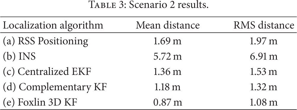
Let us start with scenario 1, whose results are summarized in Table 2. Results show that both filters are able to improve both raw RSS-based positioning and INS integration. Complementary KF has better results and is more stable than centralized KF in our deployment. Meanwhile, the results of scenario 2, included in Table 3, confirm that the filter performances do not degrade with time, which happens for INS integration. Of course, Foxlin algorithm has the best accuracy, but the difference is not so big, making our proposed filters competitive.

Table 2

Scenario 1 results.

Localization algorithm	Mean distance	RMS distance
(a) RSS positioning	1.55 m	1.80 m
(b) INS	5.24 m	5.7 m
(c) Centralized EKF	1.38 m	1.50 m
(d) Complementary KF	1.12 m	1.24 m
(e) Foxlin 3D KF	0.84 m	1.02 m

Table 3

Scenario 2 results.

Localization algorithm	Mean distance	RMS distance
(a) RSS Positioning	1.69 m	1.97 m
(b) INS	5.72 m	6.91 m
(c) Centralized EKF	1.36 m	1.53 m
(d) Complementary KF	1.18 m	1.32 m
(e) Foxlin 3D KF	0.87 m	1.08 m

The complete dataset lasts for almost three hours. In this time span, the maximum error distance error observed was 4.3 meters for the complementary filter and 5.26 meters for the centralized EKF, showing the robustness of the solution, especially for the case of the complementary filter.

Finally, it should be emphasized that a large number of the filter errors are time correlated, and the tracking filters are quite often biased due to the bias terms present in the positioning system, which are clearly visible in Figure 6 (the position measurements are biased towards the center of the figure). The system is robust enough to reduce somehow this effect, but of course this unmodeled bias tends to appear in the filter output as well.

Quite often, in localization literature the error is provided in terms of a percentage of the overall traversed distance. This is somehow inspired by the increasing error of inertial navigation systems with time. When an RSS or a similar sensor is used to aid inertial navigation, this kind of error statistic is not relevant anymore, as positioning accuracy does not degrade with time. So this statistic may be done as small as desired by just increasing the length of the scenario.

5.4. Outdoor Scenario

The proposed filters follow a loosely coupled filtering approach, which enables the use of other positioning systems such as GPS. We have made initial integration of the system with a mobile phone GPS (Nexus 4), leading to a system smoothing GPS errors. Future integration of RSS and GPS aiding would be able to guarantee continuity of walking pedestrian tracking in horizontal dimensions, for indoor and outdoor movements. Surely, some additional logic for positioning measurement selection/combination and for reduction of jumps due to mixed positioning environments would be needed, due to the different types of bias of the positioning sensors.

In Figure 10 we can see the results of the complementary Kalman filter along the real trajectory, raw GPS data, and the ideal trajectory. The initialization suffered during the GPS initial measurements for the integrated system, but afterwards, once it recovered, it worked correctly. It should be emphasized that there is a minor slope of 2% in this path, which is in an urban but quite open area. From these reduced scenarios it is difficult to derive really representative performances, as the data collection (and specially speed) was not so controlled, but the averages for this and two other simple scenarios are provided in Table 4. Note INS error is increasing with time, while GPS and complementary KF statistics are much more stable.

Table 4

Example outdoor results.

Localization algorithm	Mean distance	RMS distance
GPS positioning	8.2 m	12.6 m
INS	9.7 m	15.3 m
Complementary KF	3.2 m	4.3 m

Figure 10

Complementary KF execution in outdoor application.

5.5. Computational Load Analysis

Table 5 summarizes the amount of operations needed to process each kind of measurement received by the filter. To calculate these numbers, we have performed much optimization on the implementation of the filters as follows.

• (i)

  Many matrix coefficients are 0 or 1, and their effects in matrix summations and multiplications are well known. Therefore many operations can be avoided.

• (ii)

  Introduce the different measures received in the same time instant in order, not at the same time. This has a minor effect on the tracking quality but reduces quite much the computational needs.

• (iii)

  Reuse previously calculated terms, especially in the calculation of F matrices.

Table 5

Computational load of proposed filters for each type of measure.

Types of measure	Centralized EKF		Complementary KF
	Sums	Products	Sums	Products
Inertial, not ZVU	838	854	173	163
Position and Inertial, not ZVU	1021	1034	259	247
Inertial low speed	797	761	173	163
Position and inertial low speed	1021	1034	259	247
Inertial ZVU	610	539	302	292
Position and inertial ZVU	793	719	388	378

For computational load assessment, we will assume as negligible the load associated with the pair of cosines and sinuses that need to be computed in each of the systems.

Different types of measurements are considered in Table 5. “Inertial” measures just contain acceleration and heading (at 50 Hz rate). “position and inertial” measures contain additionally position measures derived from RSS (or GPS) in indoor scenario at 10 Hz rate. In this table we denote as “not ZVU” the measures that have not been detected as ZVU, while “ZVU” denote the measures where ZVU was detected. “Low speed” measures are the measures where ZVU were not detected, but speed is assumed to be too low and potentially problematic for the centralized EFK. Each type of measurement uses different prediction and/or filtering equations, resulting in a different number of summations and products, which have been counted for each specific case. Also, the ZVU detectors computational load was assessed.

From Table 5 it is clear that the complementary KF based system has much lower computational load. In our system, we have an update rate for position of 10 Hz and an update rate for inertial measurements of 50 Hz. From this data, assuming ZVU lasts for 35%, while low velocity lasts for 5% of the stance, it would be needed, in average, nearly 80000 FLOPS for the centralized EKF and 23000 FLOPS for the complementary EKF based integrator.

For comparison, Table 6 contains an assessment of the computational load of the complete complementary Kalman filter by Foxlin [15], which performs no simplification on the state vector, resulting in a much bigger state vector and associated covariance matrices. This solution had several phases: calibration, navigation, and so forth. The computational cost measured here would be the one related to the navigation phase, where the associated KF has 15 state variables.

Table 6

Computational load for each type of measure for Foxlin filter.

Types of measure	Foxlin complementary KF
	Sums	Products
Inertial, not ZVU	3315	3581
Position and Inertial, not ZVU	5715	6231
Inertial low speed	3315	3581
Position and inertial low speed	5715	6231
Inertial ZVU	5617	6043
Position and inertial ZVU	8017	8147

It can be seen the computational load is much higher than in our proposals, even after performing the same kinds of optimizations of the filters on Foxlin proposal. With the same measurement rates (sampling frequencies) and assumed percentage of ZVU duration this processing would demand a computational load in the order of 475000 FLOPS (which is attainable in current mobile applications, but results in increased 2000% computation/battery cost over our complementary EKF solution). This computational gain comes basically from the reduced size of the state and measurement vectors of our proposals.

It should be noted that the computational load in the IMU (which provides the heading estimate) is not computed, as we do not have access to their complete algorithms. Taking into account the size of the associated state vectors of a Kalman filter for assessing heading based on 3 axes magnetometers and gyros, a computational load in the order of that of the complementary filter could appear. This load will not be present in Foxlin filter, which operates on raw measures. This would increase our complete solution computational load, so that Foxlin solution will just have around 1000% higher computation/battery cost. Even simpler approaches could be used without the need of 3D magnetometer and gyros measurements, exploiting the flat movement restrictions.

6. Conclusions and Future Work

This paper describes the application of two novel nonlinear filters to the problem of pedestrian tracking, using low-grade positioning and inertial sensors. The filters use the measurements projected to the horizontal plane and neglect the errors introduced by the projection of gravity and foot rotation along the stance. So, the described filters track a reduced number of states with respect to other previous filters in the literature. The paper contains a comparative analysis of both solutions in a realistic indoor scenario, where the solutions show their robustness and accuracy, even though many of the error sources have been ignored: gyro bias, acceleration projection of gravity, positioning bias, and so forth.

Our study shows that the filters are capable of attaining a positioning error with an RMS in the order of 1.3–1.5 meters for long time intervals (summing nearly three hours of data), which is a level of accuracy compatible with many indoor applications; this level of accuracy does not degrade along time. Specifically, the designed complementary system seems a good solution regarding both complexity and resulting accuracy. Also, due to its design, the system would be able to maintain accuracy during short support positioning systems outages or in the reduced areas without proper positioning system coverage.

Of course, the accuracy of the system is dependent on the accuracy and measurement period of the positioning system, as shown by the difference between indoor and outdoor scenarios results (Sections 5.3 and 5.4). The exact accuracy attainable for each positioning system is not easy to derive, but for high rate sensors ( $>$ 1 measures/second) and reduced error ( $<$ 20 m RMS), a division of the RMS of the input positioning system by a factor in the range 1.5 to 3 could be expected.

The IMU that has been used in the experiments requires a connection by cable to a concentrator that the user wears attached to the belt. Obviously, this is a solution that will be difficult to generalize in commercial terms. Thus, it is needed to consider that a sound wearable system will have to send the data from the IMU to the mobile phone (processing unit) wirelessly. Reduced computational complexity will be then required to save battery. It is also needed to further study the power usage from the wireless data transfer. In our approach, some intermediate data may be calculated in the foot (i.e., “heading” from magnetometer and gyros), and not all raw measurements need to be transmitted (only 2D acceleration). Therefore, our approach reduces communication bandwidth needs and may lower the associated power consumption. These facts may underline the benefits of our approaches, although a rigorous assessment of the attainable power consumption would need to be performed. Additionally, a reduced IMU with an incomplete set of sensors could be designed, ensuring that it provides accurate heading and 2D acceleration for the application on flat movement.

Some open problems remain for the future research, as it would be the extension of the filtering approaches to running pedestrians or to other kinds of activities, and the analysis of their validity for changes of level within a building, both through stair climbing and use of elevators. Additionally, the integration of GPS must be both improved and fine-tuned, and the quality for outdoor applications must be rigorously assessed. Additionally, as described in Section 5.2, an alternative centralized EKF using acceleration measurements as control inputs could be investigated. This solution would have reduced computational cost (although larger than complementary filter) with respect to centralized EKF and similar performance.