Fault Diagnosis of Broken Rotor Bars in Squirrel-Cage Induction Motor of Hoister Based on Duffing Oscillator and Multifractal Dimension

Abstract

This paper is to propose a novel fault diagnosis method for broken rotor bars in squirrel-cage induction motor of hoister, which is based on duffing oscillator and multifractal dimension. Firstly, based on the analysis of the structure and performance of modified duffing oscillator, the end of transitional slope from chaotic area to large-scale cycle area is selected as the optimal critical threshold of duffing oscillator by bifurcation diagrams and Lyapunov exponent. Secondly, the phase transformation duffing oscillator from chaos to intermittent chaos is sensitive to the signals, whose frequency difference is quite weak from the reference signal. The spectrums of the largest Lyapunov exponents and bifurcation diagrams of the duffing oscillator are utilized to analyze the variance in different parameters of frequency. Finally, this paper is to analyze the characteristics of both single fractal (box-counting dimension) and multifractal and make a comparison between them. Multifractal detrended fluctuation analysis is applied to detect extra frequency component of current signal. Experimental results reveal that the method is effective for early detection of broken rotor bars in squirrel-cage induction motor of hoister.

1. Introduction

In recent years, large-scale hoister has been widely used in modern mine. As typical equipment of mine, hoister undertakes the lifting tasks of personnel, materials, coal, equipment, and so forth. Hoister controls the throat of coal production, and its working reliability is directly connected with the safety and stability. Hoisting system is composed of induction motor, gear reducer, drum, hydraulic braking system, multifunction digital depth system, velocity measurement system, control system, and so forth. Among them, induction motor is the power source of hoister, which plays a vital important role in the hoisting system. Because squirrel-cage induction motor is chiefly characterized by good durability, high power, low investment, heavy load, high reliability, and so forth, it has become the main choice of the driving motor in hoister. However, once the motor can not work, it will bring huge economic damage which leads to the stagnation of the entire production process or even endanger the worker's life. Among many faults of the motor, rotor bar breakage is of most serious damage and it is difficult to be found previously. If the fault of broken rotor bars (BRB) can be detected in the early stages, the serious damage can be avoided. Thus, the detection of BRB in squirrel-cage induction motor has important significance for improving the reliability of hoister.

In the hoisting process, the squirrel-cage induction motor very easily produces the fault of the broken rotor by frequent start and stop to motor under heavy load conditions. Particularly in the start-up stage of motors, the current is excessive overload in a short time, which will lead to the temperature rise and strong wallop for its stator and rotor conductors. All these finally result in forming the broken rotor bars.

Many researchers have focused their attention on fault detection of BRB during the last decades. Because the rotor of the squirrel-cage motor has no direct electrical connection, it is difficult to detect fault of BRB directly [1–4]. In order to simplify detecting conditions and improve the precision of fault diagnosis, the common method is motor current signature analysis (MCSA) [4–7]. The MCSA technique can easily detect broken rotor bars by using only current sensors; thus noninvasive detection is achieved. Compared with other detecting signals for the fault of BRB, it has many advantages in the aspects of accuracy, reliability, and conciseness [7–10]. Up to now, MCSA is applied in squirrel-cage induction motor to monitor BRB. The ideal frequency of the stator current is single; that is, the power frequency is f. Extra frequency component with (1±2s)f will appear in the frequency spectrum graph of the stator current when there is BRB fault in the motor. Therefore, through the stator current signal, we can judge whether the rotor fault occurs or not. However, the harmonic components (1±2s)f are very close to the power frequency components f, so it adds many difficulties to detect the components of fault feature frequency, which are prone to be submerged in the strong supply power frequency component in the FFT spectrum. To solve this problem, many researchers focused on studying the zoom-FFT, marginal spectrum [1], high-resolution spectrum [11], higher order spectral analysis [12], wavelet analysis [13, 14], Kalman filters, the self-adaptive filter [1], and so forth.

The rest of this paper is structured as follows. In Sections 2 and 3, the fundamental theories behind duffing oscillator and box-counting dimension and multifractal detrended fluctuation analysis have been summarized, and the proposed framework for fault detection of BRB is presented. In Section 4, multiple experimental results are presented, proving the efficiency of the proposed method. Finally, in Section 5, the conclusions are drawn and directions for future work are given.

2. Mathematical Theories of Duffing Oscillator

2.1. Duffing Oscillator

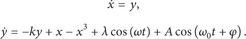
Duffing oscillator is characterized by the oscillation, forks, and chaos [15]. The dynamics equation of duffing by Holmes is described as follows:

$\ddot{x}+k\dot{x}-x+x^{\mathrm{3}}=\lambda \cos \left(\omega t\right)+s\left(t\right),$

(1)

where k is the damping constant; x³ − x is the nonlinear recovery force; λ is the amplitude of the periodic driving force; ω is the angular frequency periodic driving force; s(t) = Acos⁡(ω₀t + φ) is the signal to be detected, ω₀ is the angular frequency of s(t) and ω₀ is very close to the frequency ω, ω₀ = ω±Δω; φ is the initial phase angle of s(t); A is the amplitude of s(t).

When ω = 1 rad/s, (1) can be written as a set of state equations:

$\begin{array}{c}\dot{x}=y,\\ \dot{y}=-ky+x-x^{\mathrm{3}}+\lambda \cos \left(\omega t\right)+A\cos \left({\omega }_{\mathrm{0}}t+\phi \right).\end{array}$

(2)

All this being said, the frequency of the signal to be detected is 1 Hz or so when ω is 1 rad/s. To make the system detect the signal at any frequency, the dynamic equation of duffing by Holmes is modified in the present study, which is as follows:

$\begin{array}{c}\dot{x}=\omega y,\\ \dot{y}=\omega \left(-ky+x-x^{\mathrm{3}}+\lambda \cos \left(\omega t\right)+A\cos \left({\omega }_{\mathrm{0}}t+\phi \right)\right),\end{array}$

(3)

$\ddot{x}+k\dot{x}-x+x^{\mathrm{3}}=\lambda \cos \left(\omega t\right)+A\cos \left({\omega }_{\mathrm{0}}t+\phi \right).$

(4)

The right portion of (4) can be turned into a new equation, which is as follows:

$\begin{array}{c}\lambda \cos \left(\omega t\right)+A\cos \left({\omega }_{\mathrm{0}}t+\phi \right)=f\left(t\right)\left(t+\theta \left(t\right)\right),\\ f\left(t\right)=\sqrt{{\lambda }^{\mathrm{2}}+A^{\mathrm{2}}+\mathrm{2}\lambda A\cos \left(\Delta \omega t+\phi \right)},\\ \theta \left(t\right)=\arctan \left(\frac{A\sin \left(\Delta \omega +\phi \right)}{\lambda +A\cos \left(\Delta \omega +\phi \right)}\right),\end{array}$

(5)

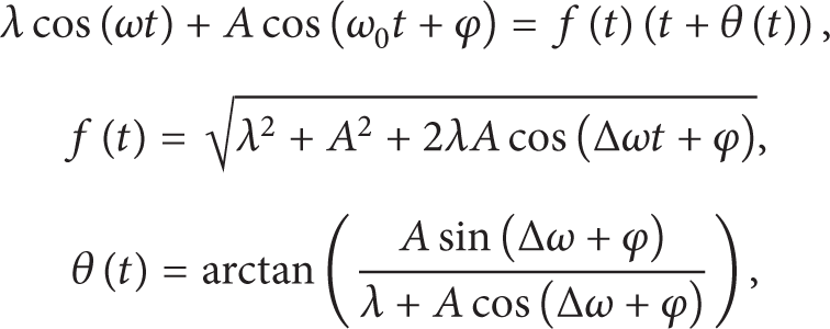
where f(t) is the total amplitude of the periodic driving force; θ(t) is the angular frequency of the total periodic driving force; because A is much less than λ, θ(t) is small enough to be ignored in this study [16].

To detect the extra frequency component of broken rotor bar, Δω is not obviously zero. Some researchers focused on studying the variables of Δω. The variances of f(t) are slow when Δω is very small. For original duffing system without s(ω₀t) in (3), when k is fixed, let λ increase gradually from zero to more than a certain threshold λ₀ and keep increasing to above another threshold λ₁; then the law of the state change of the duffing oscillator in the phase space is as follows: (1) small-scale periodic state; (2) chaotic state; (3) large-scale periodic state. Hereinto, the transformation process from chaotic state to large-scale periodic state has been widely used in character extracting of the weak signal. So the method is called backward detecting method. However, the backward detecting method is not omnipotent to deal with all weak signals. Contrary to the forward detecting method, this method is based on the transformation of the chaotic oscillator which is from the large-scale periodic state to the chaotic state. This method is called forward detecting method, which is used to detect the fault of BRB in this paper [17].

2.2. Evaluation Indexes of Duffing Oscillator

2.2.1. Bifurcation Analysis

As a control parameter, bifurcation has a qualitative change in an attractor's structure and is smoothly varied. For example, a simple equilibrium, or fixed point attractor, might give way to a periodic oscillation as the stress on a system increases. Similarly, a periodic attractor might become unstable and be replaced by a chaotic attractor. Therefore, bifurcations of duffing equation can be seen as useful information for the detection of weak signal [18].

2.2.2. Lyapunov Exponent

Lyapunov exponent (LE) is one of the most commonly used methods for determining the status of duffing system. On the calculation of LE, many methods, such as defined method, Wolf algorithm, Jacobian method, P-norm method and small data set arithmetic, are developed from the nonlinear dynamic and chaos theory [19]. The largest Lyapunov exponent is computed by using the Wolf algorithm in this study. LE measures the average rate of divergence or convergence of two neighboring trajectories in its phase space. LE may be positive or negative for the stochastic signals; that is to say, the positive Lyapunov exponent represents the divergence in the corresponding direction, and the negative LE implies the convergence in the corresponding direction. The system tends to be stable if all Lyapunov exponents are negative. The system takes periodic motion if Lyapunov exponents are zero and the other is negative. The system is in chaotic state if Lyapunov exponents have one positive value. Therefore, if the largest value in the spectrum of Lyapunov exponents is positive, it means that the system is chaotic. For duffing oscillator, the positive value of the largest Lyapunov exponent represents the fact that duffing system arrives at the chaotic state. The negative value of the largest Lyapunov exponent represents the fact that duffing system is still in the large-scale periodic state.

3. Mathematical Theories of Fractal Dimension

Dimension is one of the most important basic concepts in traditional Euclidean geometry, and the figure's dimension is always an integer. However, the dimension of some figures and signals has been proved to be noninteger. Fractal dimension is proposed to describe geometric objects that are not possible in traditional Euclidean geometry. The fractal dimension is a quantitative parameter that describes the fractal objects and indicates the complicity and essential characteristics of research object [20, 21]. At present, fractal dimension has been widely used in the areas of machine vision, image processing, surface tribology, and pattern recognition. However, the application of fractal analysis to fault diagnosis is still in its infant stages [20–23].

Fractal dimension, as a characteristic index used to quantitatively describe the complexity of signals, is characterized by the invariance under nonlinear changes. There are many calculation methods of fractal dimension, such as box-counting dimension, information dimension, capacity dimension, and correlation dimension.

3.1. Box-Counting Dimension

Let B be any non-empty compact subset of R ⁿ and let N(B,ε) be the smallest number of boxes of radius ε that cover B. Thus, the box-counting dimension is defined as follows:

$D_B=\underset{\epsilon \to \mathrm{0}}{\lim }\frac{\log N(B,\epsilon )}{\log \left(\mathrm{1}/\epsilon \right)}.$

(6)

3.2. Multifractal Detrended Fluctuation Analysis

Multifractal detrended fluctuation analysis (MF-DFA) is an extension of the detrended fluctuation analysis (DFA). MF-DFA is a powerful method which can effectively reveal the multifractality of nonstationary time series. MF-DFA, a conventional statistical method, is widely used in image processing, data mining, biological engineering, environment, fault diagnosis, and so forth.

The generalized MF-DFA procedure mainly consists of five steps [24]. In the first three steps, the procedural contents are essentially identical to the conventional DFA method. Under the assumption that the time series {x(k),k = 1, 2, …,N} is of compact support, the procedures of calculating MF-DFA are as follows.

Step 1. The calculation for the accumulated deviation series Y(i) of regarding time series x(k) to the mean value $\stackrel{-}{x}$ is

$Y\left(i\right)={\displaystyle \sum }_k^i\left[x\left(k\right)-\stackrel{-}{x}\right]\hspace{1em}(i=\mathrm{1,2},\dots ,N).$

(7)

Here $\stackrel{-}{x}$ is the mean value of x(k).

Step 2. In this step, the time series Y(i) of length N data points is mapped into m nonoverlapping segments with equal length s. Since the length N is not often evenly divisible by the time scale s, a short part at the end of the profile could not be fully used. In order to make full use of the series, 2m nonoverlapping segments can be derived through repeating the same partition procedures from the end of the series Y(i).

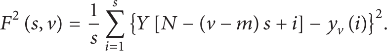
Step 3. The calculation for the local trend for each segment of the 2m segments uses the least-square fit of the series Y(i). Let us suppose that y _v (i) is the fitting polynomial in the vth segment, whether r be linear, quadratic, cubic, or higher order polynomials, it can be used in the fitting procedure. Since the order polynomials indicate the degree of the detrending of the time series in the fitting procedure, different order DFA differ in their capability of eliminating and trend in the series; namely, the higher the order is, the better the trend elimination result is and, correspondingly, the more the calculating time will be. Then determine the variance as follows.

For each segment v, v = 1, 2, …,m,

$F^{\mathrm{2}}\left(s,v\right)=\frac{\mathrm{1}}{s}{{\displaystyle \sum }}_{i=\mathrm{1}}^s{\left\{Y\left[\left(v-\mathrm{1}\right)s+i\right]-y_v\left(i\right)\right\}}^{\mathrm{2}}.$

(8)

For v = m + 1, m + 2,…,2m,

$F^{\mathrm{2}}\left(s,v\right)=\frac{\mathrm{1}}{s}{{\displaystyle \sum }}_{i=\mathrm{1}}^s{\left\{Y\left[N-\left(v-m\right)s+i\right]-y_v\left(i\right)\right\}}^{\mathrm{2}}.$

(9)

Step 4. The qth order fluctuation function F _q (s) could be worked out by the calculation of the average over all the 2m segments. The qth order fluctuation function is

$F_q\left(s\right)={\left\{\frac{\mathrm{1}}{\mathrm{2}m}{{{\displaystyle \sum }}_{v=\mathrm{1}}^{\mathrm{2}m}\left[F^{\mathrm{2}}\left(s,v\right)\right]}^{q/\mathrm{2}}\right\}}^{\mathrm{1}/q}.$

(10)

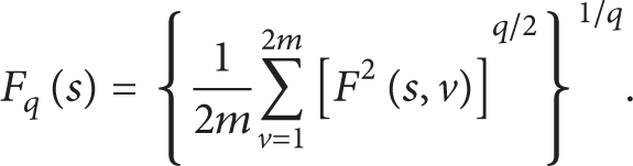
Here, the index q can be assigned with any real value. For q = 2, the traditional DFA procedure is retrieved. The physical meaning of (10) shows the different fluctuation degree of function F _q (s) for different values of q. For q ≤ 0 and |q| ≥ 1, the scales of F _q (s) mainly depend on that of small fluctuation deviation F²(s,v). Correspondingly, for q > 0 and |q| ≥ 1, the large fluctuation deviation F²(s,v) also has a decisive effect on F _q (s). Thus, with the use of polynomial fitting of each segment, the mean square error F²(s,v) can not only eliminate the trend of those small segments, but also have a great benefit to the singularity identification of the local fluctuation.

Step 5. Determine the scaling behavior of the fluctuation function F _q (s). By analyzing the logarithmic relation between F _q (s) and s, the scaling property can be determined, among which F _q (s) is a function of q and s and max⁡(k + 2, 10) ≤ s ≤ N/4, as a power-law,

$F_q\left(s\right)~s^{h\left(q\right)}.$

(11)

Generally, the fluctuation of function F _q (s) with the increment s can estimate the scaling exponent h(q) on the logarithmic diagram by fitting, which is also known as generalized Hurst exponent. If sequence is single fractal, the mean square error F²(s,v) is equivalent; thus h(q) is constant for each scaling segment. When the sequence is not related or is in a short-range correlation, the sequence is an independent random process, and h(q) = 1/2. When h(q) is nonlinearly related to q, it can be inferred that sequence exhibits multifractal properties.

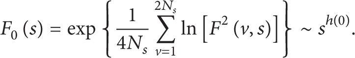
The value of h(0), which corresponds to the limit h(q) for q = 0, can not be determined directly by using the averaging procedure in (4) because of the diverging exponent. Instead, a logarithmic averaging procedure has to be employed:

$F_{\mathrm{0}}\left(s\right)=\exp \left\{\frac{\mathrm{1}}{\mathrm{4}{N}_s}{{\displaystyle \sum }}_{v=\mathrm{1}}^{\mathrm{2}{N}_s}\ln \left[F^{\mathrm{2}}\left(v,s\right)\right]\right\}~s^{h\left(\mathrm{0}\right)}.$

(12)

Once MF-DFA is applied, Step 3 can be omitted. And it is equivalent to traditional fluctuation analysis. Steps 1 and 2 of fluctuation analysis are the same as those of MF-DFA, while (8) in Step 3 is changed into

$F_{\text{FA}}^{\mathrm{2}}\left(s,v\right)={\left[Y\left(vs\right)-Y\left(\left(v-\mathrm{1}\right)s\right)\right]}^{\mathrm{2}}.$

(13)

Inserting (12) into (10) and (11), (13) can be derived:

${\left\{\frac{\mathrm{1}}{\mathrm{2}m}{{\displaystyle \sum }}_{v=\mathrm{1}}^{\mathrm{2}m}{\left[Y\left(vs\right)-Y\left(\left(v-\mathrm{1}\right)s\right)\right]}^q\right\}}^{\mathrm{1}/q}~s^{h\left(q\right)}.$

(14)

To simplify the calculation, we can assume that the length N of the series is an integer multiple of the scales, namely, m = N/s. Take the simple condition for instance. For N is integer multiple of s, namely, m = N/s, so

${{\displaystyle \sum }}_{v=\mathrm{1}}^m{\left|Y\left(vs\right)-Y\left(\left(v-\mathrm{1}\right)s\right)\right|}^q~s^{qh\left(q\right)-\mathrm{1}}.$

(15)

And the following formula can be derived from (8):

$\left|Y\left(vs\right)-Y\left(\left(v-\mathrm{1}\right)s\right)\right|={{\displaystyle \sum }}_{k=(v-\mathrm{1})s}^{vs}{x}_k=P_s\left(v\right).$

(16)

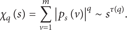
The definition of the scaling exponent τ(q) is based on the partition function χ _q (ε); the relation is as follows:

${\chi }_q\left(s\right)={{\displaystyle \sum }}_{v=\mathrm{1}}^m{\left|p_s\left(v\right)\right|}^q~s^{\tau \left(q\right)}.$

(17)

Based on (14) to (16), the relations between the generalized Hurst exponent h(q) and the scaling exponent τ(q) from the standard partition function can be acquired:

$\tau \left(q\right)=qh\left(q\right)-\mathrm{1}.$

(18)

To describe a multifractal series better, based on the singularity exponent α and the multifractal singularity spectrum f(α), a set of formulas is developed through a Legendre transform in statistical physics. The formulas are as follows:

$\begin{array}{c}\alpha \left(q\right)=\frac{d\tau \left(q\right)}{d\left(q\right)},\\ f\left(\alpha \right)=q\alpha \left(q\right)-\tau \left(q\right).\end{array}$

(19)

Based on (18) and (19), the relations between α and f(α) to h(q) can be inferred:

$\begin{array}{c}\alpha \left(q\right)=h\left(q\right)+\frac{qdh\left(q\right)}{d\left(q\right)},\\ f\left(\alpha \right)=q\left[\alpha \left(q\right)-h\left(q\right)\right]+\mathrm{1}.\end{array}$

(20)

For the time series are single fractal, the multifractal spectrum will be a constant. While the time series are multifractal, the multifractal spectrum will always be a unimodal bell-shaped image in contrast. The segment of f(α) ≥ 0 can be referred to as [α _min ,β_max].

MF-DFA, an extension of monofractal DFA, is a powerful tool for uncovering the nonlinear dynamical characteristics buried in nonstationary time series and can capture minor changes of complex system conditions.

4. Numerical Simulations

In the previous sections, we have focussed our study on the fundamental theory of duffing oscillator and fractal dimension, and the detecting method for recognising and predicting of the broken rotor bars was presented. In this section, what should be pointed out are the characteristics when weak external periodic signals are introduced into duffing oscillator, such as phase plane trajectories, bifurcation diagrams, and the largest Lyapunov exponents. At the end of the section, the classification performances of duffing oscillator in tandem with the fractal dimensions are used to recognize the fault of broken rotor bars.

The fault characteristic signals of broken rotor bars are displayed as side bands on the two sides of the power frequency in its frequency spectrum. Moreover, along with the decrease of the amplitude of the side band, the frequency spectrum can not recognize the fault finally.

In order to simulate the signal superposition, an analytical mathematical model is constructed. We denote

$s\left(n\right)=A_{\mathrm{0}}\cos \left(\frac{\mathrm{2}\pi nf}{f_s}\right)+A_{\mathrm{1}}\cos \left(\frac{\mathrm{2}\pi n{f}_{\mathrm{1}}}{f_s}\right).$

(21)

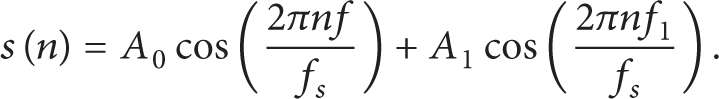
Here the sampling frequency is f _s = 500 Hz, the number of the sampling points is n = 2048, A₀ = 1, A₁ = 0.02, the synchronous speed is n₀ = 1500 rpm, the measured speed is n₁ = 1485 rpm at no load condition, the slip ratio is s = (n₀ − n₁)/n₀ = 0.01, the power frequency is f = 50 Hz, and the frequency component of BRB is f₁ = (1 − 2s)f = 49 Hz.

4.1. Numerical Simulations of Bifurcation

The parameters of duffing oscillator can be represented by the fixed values, such as k = 0.5 and A = 0.02, and let λ increase gradually from zero to achieve a certain threshold λ = 1. Figure 1 shows the bifurcation diagrams of duffing oscillator obtained by varying λ from 0 to 1 under the prerequisite of the different frequencies. The differences of the first bifurcation diagram in Figure 1(a) and other bifurcation diagrams such as Figures 1(b)–1(f) can be obviously seen. As λ is increased from zero, a stable period orbit occurs, which persists up to λ = 0.359 and then it loses its stability and gives birth to a new period orbit. The chaotic motion suddenly disappears at λ = 0.825 in Figure 1(a). Compared with Figure 1(a), the other bifurcation diagrams have intermittent concussion in the early orbit and later orbit, as well as the chaotic motion with longer time. The thresholds of the chaotic oscillator from chaotic state to the large-scale periodic state then can be explained, as shown in Table 1.

Table 1:

Bifurcation thresholds of the chaotic oscillator from chaotic state to the large-scale periodic state diagram.

Δω	0	±0.01	±0.02	±0.03	±0.04	±0.05
λ	0.825	0.864	0.864	0.863	0.862	0.862

Figure 1:

Bifurcation diagrams of the duffing oscillator in different parameters: (a) Δω = 0, (b) Δω = ±0.01, (c) Δω = ±0.02, (d) Δω = ±0.03, (e) Δω = ±0.04, and (f) Δω = ±0.05.

4.2. Numerical Simulations of the Largest Lyapunov Exponents

The spectrums of the largest Lyapunov exponents are used to describe the states of duffing oscillator. Numerical simulations show that the corresponding diagrams of the largest Lyapunov exponents are given in Figure 2. The spectrums of the largest Lyapunov exponents corresponding to Δω and λ are shown in Table 2. The result shows that the threshold of the forward detecting method is generally larger with the increase of the extra frequencies Δω. Therefore, based on the above mentioned reasons, the detecting method of BRB sets λ = 0.83 as the marking threshold.

Table 2:

The thresholds of the chaotic oscillator from chaotic state to the large-scale periodic state by using the largest Lyapunov exponents.

Δω	0	±0.01	±0.02	±0.03	±0.04	±0.05
λ	0.82550	0.83890	0.86266	0.86154	0.86180	0.86188

Figure 2:

The largest Lyapunov exponent diagrams of the duffing oscillator in different parameters: (a) Δω = 0, (b) Δω = ±0.01, (c) Δω = ±0.02, (d) Δω = ±0.03, (e) Δω = ±0.04, and (f) Δω = ±0.05.

4.3. Numerical Simulations of Duffing Oscillator

When Δω = 0, the output current signal and the phase plane trajectories of normal motor from the duffing oscillator are given in Figures 3(a) and 3(b). In order to observe the details of the output current signal x through the duffing oscillator, we only render the early-stage visible parts of the entire output current signal in Figure 3(a). When Δω = 0.02, the output current signal and the phase plane trajectories of normal motor with BRB from the duffing oscillator are given in Figures 3(c) and 3(d). However, Figure 3(b) shows that the output current signal of duffing oscillator has obvious periodic oscillation. Owing to the difference of the angular frequency Δω, the phase plane trajectories are different. Figure 3(c) shows that the duffing oscillator is yet in the large-scale periodic state. But Figure 3(d) shows that the duffing oscillator is still in chaotic state. Therefore, based on the results mentioned above, it has been proven in simulation to be an effective detecting method of BRB.

Figure 3:

Time response and phase plane trajectories of the duffing oscillator in different conditions. (a) The current signal of normal motor, (b) the current signal of motor with broken rotor bars, (c) the phase plane trajectories of normal motor, and (d) the phase plane trajectories of motor with broken rotor bars.

4.4. Numerical Simulations of Box-Counting Dimension

In this section, we first analyze the dimensions by using fractal theory. As shown in Figure 3(c), the output current signal of motor with broken rotor bars from the duffing oscillator is chiefly characterized by fractal. Figure 4 displays the box-counting dimension of the output current signal of the duffing oscillator under different conditions: (a) the current signal of normal motor and (b) the current signal of motor with BRB. There are prominent differences between normal current signal and current signal of BRB in box-counting dimension. On the other hand, whether the dimension jump occurs or not depends on the output signal x of duffing oscillator.

Figure 4:

Box-counting dimension of the output current signal of the duffing oscillator in different conditions. (a) Normal current signal and (b) current signal of BRB.

4.5. Numerical Simulations of MF-DFA

In this subsection, multifractality of two output signals is utilized to analyze fault diagnosis of BRB in squirrel-cage induction motor by MF-DFA. The index q in MF-DFA was uniformly set to range from negative ten to positive ten with the increment unity. Figure 5(a) depicts the time domain containing two different output currents from duffing oscillator. Figures 5(a)–5(d) depict the generalized Hurst exponents, the scaling exponents, and the multifractal spectra of two such groups of data as that in Figure 5(a). As shown in Figure 5, normal current signal is also significantly different from current signal of BRB. MF-DFA method can extract the fault of broken rotor bars. The result shows that the MF-DFA method can provide more different information than by only using duffing oscillator or box-counting dimension.

Figure 5:

Multifractal detrended fluctuation analysis of two current signals in the same signal processing from duffing oscillator for q = − 10:0.3:10. (a) The comparison of different current signals, (b) the generalized Hurst exponent H(q), (c) the scaling exponent τ(q), and (d) the multifractal spectrum f(α).

5. Conclusions

According to the requirement of accurate detection for broken rotor bars in squirrel-cage induction motor of hoister, a novel method which is based on duffing oscillator and multifractal dimension is proposed in this paper. Through the simulation of the fault signal model with broken rotor bars, the results of the research are demonstrated as follows. Firstly, based on the analysis of the structure and performance of the modified duffing oscillator, the end of transitional slope from chaotic area to large-scale cycle area is selected as the optimal critical threshold of duffing oscillator by bifurcation diagrams and Lyapunov exponent. Secondly, aiming at the range of harmonic component (1±2s)f, different parameters Δω are also considered as variables. Finally, MF-DFA method can extract the fault of broken rotor bars and have a better recognition result than by only using duffing oscillator or box-counting dimension. Because of the application of duffing oscillator and MF-DFA, considerable achievements have been obtained.

Conflict of Interests

The authors declare that there is no conflict of interests regarding the publication of this paper.