Sage Journals: Discover world-class research

Abstract

Accurately predicting hydraulic characteristics in the charge-up process of horizontal pipeline with entrapped air pocket is of great significance for the process design and field operation of the oil pipeline commissioning. In this paper, this process is simulated and its hydraulic characteristics are analyzed. Finite difference method and characteristic method are combined to obtain the velocity and pressure field of the whole line. Results show that when air pockets reach the outlet of the pipeline, they blow out tempestuously and the velocity of gas may reach tens times of its normal flow velocity. At the beginning and end of the blowing out, velocity and pressure of the whole line suffer acute change. Based on this, the influence of several critical parameters is compared and analyzed by several groups of examples.

1. Introduction

Pipeline commissioning is a critical stage connecting construction and daily operation. In recent years, with the construction and operation of a large number of pipelines in China and abroad, problems encountered in the pipeline commissioning process have attracted more and more attention.

Among all the commissioning methods, direct commissioning has become a mainstream one due to its time efficiency and low cost. During the process of direct commissioning, before the oil is pumped into pipeline, some preparation work, such as hydraulic test and pipeline internal cleaning, has to be performed. However, during the cleaning process, it is impossible to remove all water remaining from hydraulic test. Therefore, there is still a considerable amount of residual water in pipeline after the cleaning process. The residual water is pushed and gathered by the pig placed just before the oil front which acts as an isolator and cleaner and thus is forced to flow in front of the pig and the flow eventually evolves into air-water two-phase flow. Considering the complex flow circumstance in the pipeline, entrapped air pockets will inevitably form due to the self-instability of fluid. Once the entrapped air pocket forms, on account of the compressibility of air and interaction between gas phase and liquid phase, the existence of the air pocket may bring threat to the commissioning operation and thus its hydraulic characteristics have to be well understood.

At present, there are few studies on the commissioning process. However, the study on the charge-up process of the pipeline with entrapped air can be used for reference. Zhang and Vairavamoorthy [1, 2] established a mathematical model for the charge-up process in an air-entrapped pipeline with moving boundary conditions. A coordinate transformation technique was employed to reduce fluid motion in time-dependent domains to one in time-independent domains. This study was confined to model transient flow in a filling pipeline with only one entrapped air pocket and thus not typical enough. Jiang et al. [3] proposed a mathematical model to describe the flow behavior in the pipeline and predicted pressure transients accompanying gas bubbles and cavitation inside low pressure pipeline in hydraulic system. Liu and Suo [4] introduced a rigid mathematical model to simulate the behavior of the entrapped air pocket and presented the governing equations of the air pocket, liquid slug, and liquid-gas interface. Yang et al. [5] established a mathematical model for describing the water-filling process based on Preissmann implicit difference method. The whole process including the transition from initial empty state to free surface flow and the transition from free surface flow to pressurized flow was analyzed. However, the result that this study obtained was applicable to only a few boundary conditions.

In this paper, critical process of commissioning is simulated. To solve the problem that pressure and velocity on the gas-liquid interface are hard to couple and flow parameters at the inlet and outlet fluctuates severely, which makes calculation difficult to converge, the approach combining finite difference method and characteristic method is adopted to perform an iterative calculation of the flow parameters along the whole pipe section. By monitoring inlet velocity, gas-liquid interface location, and blowing out process of air pockets in a series of typical examples, hydraulic characteristics and critical influencing factors are analyzed in order to provide more accurate reference and evidence for the process design and field operation of the practical commissioning process.

2. Physical Model

In the practical commissioning process, the actual volume and location of the residual water are very difficult to predict. The flow circumstance of the pipeline in commissioning is so complex that it is very difficult to simulate the distribution state of air pockets. Meanwhile, in engineering practice, what is concerned mostly is the flow parameters fluctuation when air pockets reach the outlet, such as the impact on downstream facilities caused by their blowing out. Based on this, this paper focuses on the hydraulic characteristics after air pockets have been formed. Practical process is simplified as follows.

As direct commissioning is usually performed at normal temperature, thermal influence is not considered.

Considering the engineering background of the problem and the limitation of computation amount, three-dimensional problem is simplified into one-dimensional problem.

Air pockets have been formed before the simulation; thus their distribution state is known and given.

As the phase transition such as evaporation is not considered, air pocket is constituted of pure air, which is considered as ideal gas.

The interface between water and air is vertical to the pipeline axis.

The elasticity of pipe wall and water is neglected.

Based on these assumptions, the practical commissioning process is necessarily and reasonably simplified into the physical model as Figure 1 shows.

Figure 1:

Schematic of physical model.

In the following section of this paper, mathematical model is established corresponding to this physical model and numerical method is used to perform a transient simulation of the commissioning process.

3. Mathematical Method

3.1. Governing Equations

(1) Governing Equations for the Liquid Phase.Differential equation of motion for the liquid phase is

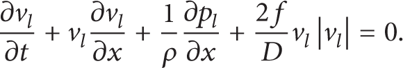
\frac{\partial v_{l}}{\partial t} + v_{l} \frac{\partial v_{l}}{\partial x} + \frac{1}{ρ} \frac{\partial p_{l}}{\partial x} + \frac{2 f}{D} v_{l} | v_{l} | = 0 .

(1)

Differential equation of continuity for the liquid phase is

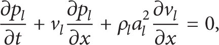
\frac{\partial p_{l}}{\partial t} + v_{l} \frac{\partial p_{l}}{\partial x} + ρ_{l} a_{l}^{2} \frac{\partial v_{l}}{\partial x} = 0,

(2)

where ρ_l is liquid density, kg/m³; v_l is liquid flow velocity, m/s; p_l is liquid pressure, Pa; a_l is liquid pressure wave velocity, m/s; D is pipeline inner diameter, m; f is friction coefficient, dimensionless.

(2) Governing Equations for the Gas Phase. Differential equation of motion for the gas phase is

\frac{\partial v_{g}}{\partial t} + v_{g} \frac{\partial v_{g}}{\partial x} + \frac{2}{γ - 1} a_{g} \frac{\partial a_{g}}{\partial x} = 0 .

(3)

Differential equation of continuity for the gas phase is

\frac{\partial a_{g}}{\partial t} + v_{g} \frac{\partial a_{g}}{\partial x} + \frac{γ - 1}{2} a_{g} \frac{\partial v_{g}}{\partial x} = 0,

(4)

where γ is polytropic exponent, assigned value 1.2 in this paper; v_g is gas flow velocity, m/s; p_g is gas pressure, Pa; a_g is gas pressure wave velocity, m/s.

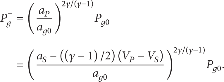
(3) Closure Equation. For the isentropic flow of ideal gas as the situation that this paper involves, gas pressure and pressure wave velocity satisfy the following relationship:

{(\frac{a_{g}}{a_{g 0}})}^{2} = {(\frac{p_{g}}{p_{g 0}})}^{2},

(5)

where a_g0 is the gas pressure wave velocity of the initial time, m/s; p_g0 is gas pressure of the initial time, Pa.

Pressure wave velocity of the initial time can be obtained by the following equation:

a_{g 0} = \sqrt{\frac{γ R T_{0}}{m_{g}}},

(6)

where R is ideal gas state constant, R = 8.3124 J/(mol·K); m_g is average molecular weight of the gas phase, set to be 28.95 g/mmol; T₀ is gas temperature in the initial time, assigned value 293.15 K.

3.2. Solving Method

3.2.1. Discretization of Computational Domain

For the commissioning charge-up process that this paper concerns, the traditional method that discretizes the computational domain by establishing fixed grid on it is not applicable. This is due to the following reasons. (1) As the gas-liquid interface moves forward continuously, its location most likely may not coincidentally overlap with the fixed grid nodes. Thus, the two critical parameters, pressure and velocity, on the interface cannot be solved accurately. (2) If fixed grid is adopted, the fluctuation of gas pressure may aggravate the convergence difficulty of the whole simulating process and even leads to divergence in some wicked boundary conditions. Therefore, this paper adopts a new grid system which combines fixed grid and moving grid. Moving grid is established on the fluid and moves with it, which is used for hydraulic calculation of pressure and velocity of the whole line at every time step. As the fluid flows in and out of the pipeline continuously, grid is updated instantly according to the immediate location of the liquid and gas. Thus, with the instant regeneration of the moving grid, the numerical process is more veritable and credible. Besides, it eliminates the discontinuity on the interface and ensures the convergence of the calculation. Meanwhile, fixed grid is established on the pipeline to save and output variable value of the whole line. Velocity and pressure values of the two grids are transferred by linear interpolation.

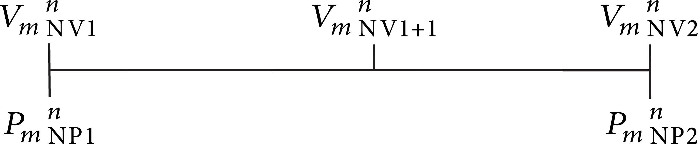
The velocity node and pressure node of moving grid are staggered. Taking the first liquid segment as an example, the moving grid system at the nth and the (n + 1) th time step are as Figure 2 shows. It is noteworthy that the value of the spatial steps of the two grids is mutually independent and the spatial step of moving grid is instantly updated according to the immediate location of liquid segment and air pocket.

Figure 2:

Moving grid system for velocity and pressure of the first liquid segment at the nth and (n + 1) th time instant.

In Figure 2, subscript m denotes moving grid, $V_{m}_{i}^{n}$ denotes the ith velocity node on the moving grid at the nth time instant, $P_{m}_{i}^{n}$ represents the ith pressure node on the moving grid at the nth time instant, and NV1 and NP1, respectively, stand for the number of velocity and pressure nodes of the first liquid segment. What needs to be notified is that NV1 and NP1 are not necessarily equal.

The velocity and pressure nodes of fixed grid are collocated. The fixed grid system is as Figure 3 shows.

Figure 3:

Fixed grid system for velocity and pressure.

In Figure 3, subscript f denotes fixed grid, V_fⁱ denotes the ith velocity node on the fixed grid, P_fⁱ represents the ith pressure node on the fixed grid, and NF stands for the number of velocity node and pressure node.

3.2.2. Discretization of Governing Equations

Take the situation that single air pocket is entrapped in pipeline as example to notify the discretization method of liquid and gas governing equations.

(1) Solution of the Internal Nodes. Discretize the equations by implicit format of finite difference method. The velocity and pressure nodes on the moving grid are staggered. Thus, the relationship between the number of pressure nodes and its neighboring velocity nodes is not always the same for every fluid segment. For example, on the first liquid segment, numbers of the neighboring nodes of the ith pressure node are i and i + 1, respectively, but those on the air pocket are i + 1 and i + 2, respectively. Thus, it is necessary to discretize the governing equations of every fluid segment, respectively.

(1.a) Discretization of the First Liquid Segment Governing Equations. Grid on the first liquid segment is as Figure 4 shows. Liquid motion equation (1) and continuity equation (2) are discretized, respectively, and rearranged into the following forms:

\begin{array}{l} V_{i}^{n + 1} = {\begin{matrix} V_{i}^{n} - [V_{i}^{n + 1} \frac{3 \times V_{i}^{n + 1} + V_{i + 1}^{n + 1} - 4 \times V_{i - 1}^{n + 1}}{Δ x} \\ + \frac{1}{ρ} \frac{P_{i}^{n + 1} - P_{i - 1}^{n + 1}}{Δ x} + \frac{2 f}{D} V_{i}^{n + 1} | V_{i}^{n + 1} |] \times Δ t \\ (i = 1) \\ V_{i}^{n} - [V_{i}^{n + 1} \frac{V_{i}^{n + 1} - V_{i - 1}^{n + 1}}{Δ x} \\ + \frac{1}{ρ} \frac{P_{i}^{n + 1} - P_{i - 1}^{n + 1}}{Δ x} + \frac{2 f}{D} V_{i}^{n + 1} | V_{i}^{n + 1} |] \times Δ t \\ (1 < i < NV 1 - 1) \\ V_{i}^{n} - [V_{i}^{n + 1} \frac{4 \times V_{i + 1}^{n + 1} - V_{i - 1}^{n + 1} - 3 \times V_{i}^{n + 1}}{Δ x} \\ + \frac{1}{ρ} \frac{P_{i}^{n + 1} - P_{i - 1}^{n + 1}}{Δ x} + \frac{2 f}{D} V_{i}^{n + 1} | V_{i}^{n + 1} |] \times Δ t \\ (i = NV 1 - 1) \end{matrix} \\ P_{i}^{n + 1} = P_{i}^{n} - [\frac{V_{i}^{n + 1} + V_{i + 1}^{n + 1}}{2} \frac{P_{i}^{n + 1} - P_{i - 1}^{n + 1}}{Δ x} + ρ a^{2} \frac{V_{i + 1}^{n + 1} - V_{i}^{n + 1}}{Δ x}] \times Δ t (0 < i < NP 1) . \end{array}

(7)

Figure 4:

Grid system of the first liquid segment.

(1.b) Discretization of the Air Pocket Governing Equations. Due to the compressibility of gas and the fact that air pocket continuously flows out of the pipeline till exhaustion, the total number of the nodes on it may reduce to 1, which needs to be considered separately.

(1.b. 1) The Situation When Total Nodes Number Is Greater than 1. In this situation, grid system in the air pocket is as Figure 5 shows. Gas motion equation (3) and continuity equation (4) are discretized, respectively, and rearranged into the following forms:

\begin{array}{l} V_{i}^{n + 1} = {\begin{matrix} V_{i}^{n} - [V_{i}^{n + 1} \frac{3 \times V_{i}^{n + 1} + V_{i + 1}^{n + 1} - 4 \times V_{i - 1}^{n + 1}}{Δ x} \\ + \frac{2}{γ - 1} \frac{a_{i - 1}^{n + 1} + a_{i - 2}^{n + 1}}{2} \frac{a_{i - 1}^{n + 1} - a_{i - 2}^{n + 1}}{Δ x}] \times Δ t \\ (i = NV 1 + 1) \\ V_{i}^{n} - [V_{i}^{n + 1} \frac{V_{i}^{n + 1} - V_{i}^{n + 1}}{Δ x} \\ + \frac{2}{γ - 1} \frac{a_{i - 1}^{n + 1} + a_{i - 2}^{n + 1}}{2} \frac{a_{i - 1}^{n + 1} - a_{i - 2}^{n + 1}}{Δ x}] \times Δ t \\ (NV 1 + 1 < i < NV 2 - 1) \\ V_{i}^{n} - [V_{i}^{n + 1} \frac{4 \times V_{i + 1}^{n + 1} - V_{i - 1}^{n + 1} - 3 \times V_{i}^{n + 1}}{Δ x} \\ + \frac{2}{γ - 1} \frac{a_{i - 1}^{n + 1} + a_{i - 2}^{n + 1}}{2} \frac{a_{i - 1}^{n + 1} - a_{i - 2}^{n + 1}}{Δ x}] \times Δ t \\ (i = NV 2 - 1) \end{matrix} \\ a_{i}^{n + 1} = a_{i}^{n} - [\frac{V_{i + 1}^{n + 1} + V_{i + 2}^{n + 1}}{2} \frac{a_{i}^{n + 1} - a_{i - 1}^{n + 1}}{Δ x} + \frac{γ - 1}{2} a_{i}^{n + 1} \frac{V_{i + 2}^{n + 1} - V_{i + 1}^{n + 1}}{Δ x}] \times Δ t (NP 1 < i < NP 2) . \end{array}

(8)

Figure 5:

Grid system of air pocket when total nodes number is greater than 1.

(1.b. 2) The Situation When Total Nodes Number Equals 1. In this situation, grid on the air pocket is as Figure 6 shows. Obviously, discretization result is as follows:

V_{i}^{n + 1} = V_{i}^{n} - [V_{i}^{n + 1} \frac{V_{i + 1}^{n + 1} - V_{i - 1}^{n + 1}}{Δ x} + \frac{2}{γ - 1} \frac{a_{i - 1}^{n + 1} + a_{i - 2}^{n + 1}}{2} \frac{a_{i - 1}^{n + 1} - a_{i - 2}^{n + 1}}{Δ x}] \times Δ t .

(9)

Figure 6:

Grid system of the air pocket when total nodes number equals 1.

(1.c) Discretization of the Second Liquid Segment Governing Equations. Similar to the air pocket, total node number of the second liquid segment also may reduce to 1. The specific discretization method is similar to that of the first liquid segment and air pocket and is not given here for brevity.

(2) Solution of the Boundary Node. In the above section, velocity and pressure values of the internal nodes are solved by finite difference method. However, for the boundary nodes, such as the inlet, outlet, and the liquid-gas interface, this method is not applicable. Thus, it is necessary to find another method to solve the value on these particular locations.

Among all the numerical methods for pipeline transient flow, characteristics method fully considers the fluid property and flow state of both sides of the liquid-gas interface. Therefore, this method ensures the equilibrium of the velocity and pressure on the interface and thus makes calculation result better conform to the physical meaning. Meanwhile, characteristics method is compatible with various boundary conditions. Based on the above advantages, characteristics method is adopted to solve the pressure and velocity values of the boundary nodes.

(2.a) Discretization of the Characteristic Equations

(2.a. 1) Discretization of the Liquid Characteristic Equations. Calculation grid of characteristic method is as Figure 7 shows. The discretization result of the characteristic equation is as follows:

P_{P} = R_{A} - S_{A} V_{P}, P_{P} = R_{B} + S_{B} V_{P},

(10)

where

\begin{matrix} R_{A} = P_{R} + ρ a V_{R}, S_{A} = ρ a (1 + \frac{2 f}{D} | V_{R} | (t_{P} - t_{R})), \\ R_{B} = P_{S} - ρ a V_{S}, S_{B} = ρ a \times (1 + \frac{2 f}{D} | V_{S} | (t_{P} - t_{R})) . \end{matrix}

(11)

Figure 7:

Calculation grid for characteristic method.

Location of point R and S is determined by

\begin{matrix} x_{R} = x_{P} - a_{R} (t_{P} - t_{R}), \\ x_{S} = x_{P} - a_{S} (t_{P} - t_{S}) . \end{matrix}

(12)

By solving these linear equations, the pressure and velocity values of next time instant can be obtained. If the location of point R and S does not just overlap with that of any grid node, their values can be obtained by interpolation.

(2.a. 2) Discretization of the Gas Characteristic Equations. Similar to the liquid characteristic equations, the following equations are obtained:

C_{W} a_{P} + V_{P} = Q_{R},

(13)

C_{W} a_{P} - V_{P} = Q_{S},

(14)

where

\begin{array}{l} C_{W} = \frac{2}{γ - 1}, \\ Q_{R} = \frac{2}{γ - 1} a_{R} + V_{R}, \\ Q_{S} = \frac{2}{γ - 1} a_{S} - V_{S} . \end{array}

(15)

(2.b) Solution of the Liquid-Gas Back Interface. In this paper, for brevity, the following naming rules are defined right now. The direction pointing from inlet to outlet is called “front” direction and the opposite one is called “back” direction. Thus, between the two interfaces of an air pocket, the one near the outlet is called “front interface” and the one near the inlet is called “back interface.” Thus, the front side of the back interface is gas and the back side of it is liquid. To obtain the velocity and pressure values on this interface, liquid C⁺ characteristic equation and gas C⁻ characteristic equation should be synthesized.

Through liquid C⁺ characteristic equation, the following relationship can be obtained:

P_{l}^{+} = R_{A} - S_{A} V_{P} = (P_{R} + ρ a V_{R}) - ρ a (1 + \frac{2 f}{D} | V_{R} | (t_{P} - t_{R})) \times V_{P} .

(16)

From gas C⁻ characteristic equation, the following relationship can be obtained:

a_{P} = \frac{Q_{S} + V_{P}}{C_{W}} = a_{S} - \frac{γ - 1}{2} (V_{P} - V_{S}) .

(17)

Substituting (16) and (17) into (5), the following relationship is obtained:

\begin{array}{l} P_{g}^{-} = {(\frac{a_{P}}{a_{g 0}})}^{2 γ / (γ - 1)} P_{g 0} \\ = {(\frac{a_{S} - ((γ - 1) / 2) (V_{P} - V_{S})}{a_{g 0}})}^{2 γ / (γ - 1)} P_{g 0} . \end{array}

(18)

Obviously, velocity and pressure values on the interface satisfy the following relationship:

P_{l}^{+} = P_{g}^{-}, V_{l}^{+} = V_{g}^{-} .

(19)

Thus, the following relationship is obtained:

{(\frac{a_{S} - ((γ - 1) / 2) (V_{P} - V_{S})}{a_{g 0}})}^{2 γ / (γ - 1)} P_{g 0} = P_{R} + ρ a (V_{R} - V_{P} + (t_{R} - t_{P}) \frac{2 f}{D} V_{P} | V_{R} |) .

(20)

Equation (20) is solved by bisection method. When velocity on the interface is obtained, it is substituted into liquid C⁺ characteristic equation to obtain the pressure value.

(2.c) Solution of the Liquid-Gas Front Interface. The front side of the front interface is liquid and the back side of it is gas. To solve the pressure and velocity on it, similar approach is adopted to obtain the following relationship:

{(\frac{((γ - 1) / 2) (V_{P} - V_{R}) + a_{R}}{a_{g 0}})}^{2 γ / (γ - 1)} P_{g 0} = P_{S} + ρ a (V_{P} - V_{S} + (t_{P} - t_{R}) \frac{2 f}{D} V_{P} | V_{S} |) .

(21)

Equation (21) is solved by bisection method. When velocity on the interface is obtained, it is substituted into liquid C⁻ characteristic equation to obtain the pressure value.

(2.d) Solution of the Pipeline Inlet. In the typical commissioning situation, inlet of the pipeline can be seen as constant-pressure inlet. The fluid that flows into the pipeline is always liquid. Thus, liquid C⁻ characteristic equation and the given inlet pressure should be synthesized to solve the inlet velocity.

Substitute the constant inlet pressure into the liquid C⁻ characteristic equation and the following equation is obtained:

P_{STA} = R_{B} + S_{B} V_{P} .

(22)

Rearrange the above equation into the following form:

V_{P} = \frac{P_{STA} - R_{B}}{S_{B}} = \frac{(P_{STA} - P_{S}) + ρ a V_{S}}{ρ a (1 + (t_{P} - t_{R}) (2 f / D) | V_{S} |)} .

(23)

Thus, the inlet velocity is obtained.

(2.e) Solution of the Pipeline Outlet. In practical commissioning situation, the residual fluid in pipeline is directly discharged into oil tank. In this paper, outlet is simplified into a constant-pressure one, which is the most similar to the practical situation. Thus, when liquid is discharged from the outlet, liquid C⁺ characteristic equation and the given constant outlet pressure should be synthesized to solve the outlet velocity. The result is as follows:

V_{P} = \frac{R_{A} - P_{E}}{S_{A}} = \frac{ρ a V_{R} - (P_{E} - P_{R})}{ρ a (1 + (t_{P} - t_{R}) (2 f / D) | V_{R} |)} .

(24)

Similarly, when gas is discharged, gas C⁺ characteristic equation and the given outlet pressure should be synthesized to solve the outlet velocity. The result is as follows:

V_{P} = Q_{R} - C_{W} a_{P} = V_{R} - \frac{2}{γ - 1} (a_{P} - a_{R}) .

(25)

With the above discretized calculation domain and equations, transient simulation can be performed by coding. Concrete calculation process is shown in Figure 8.

Figure 8:

Calculation diagram.

4. Results and Analysis

4.1. Transient Simulation of the Commissioning Charge-Up Process

In the above part of this paper, practical commissioning process is reasonably simplified to a physical model. Governing equations and their discretization method are introduced. In the subsequent part, hydraulic characteristics of this process are further analyzed by several typical examples based on the engineering practice. Taking the situation that two air pockets are entrapped in the pipeline as an example, the case described by Table 1 is designed.

Table 1:

Parameters of the case.

Parameter item	Parameter value

Pipeline length (m)	1000
Pipeline diameter (mm)	175
Pipeline inlet pressure (MPa)	0.3
Pipeline outlet pressure (MPa)	0.2
Liquid density (kg/m³)	997.0
Liquid dynamic viscosity (×10⁻⁴ Pa·s)	8.94
Liquid pressure wave velocity (m/s)	1000
Gas relative molecular mass (g/mmol)	28.95
Initial air pocket location (m, m)	(250, 400)* and (700, 850)
Time step (s)	0.01
Spatial step (m)	10
Total simulation time (s)	500

(250, 400)* The distance from the two ends of the air pocket to the inlet is 250 m and 400 m, respectively.

For the sake of convenience, following convention is made. In the situation that two air pockets are entrapped, the one near the inlet is called “back air pocket” and the one near the outlet is called “front air pocket.” From inlet to outlet, the three liquid segments are called first, second, and third.

Simulate the process by the method introduced above and the following result is obtained.

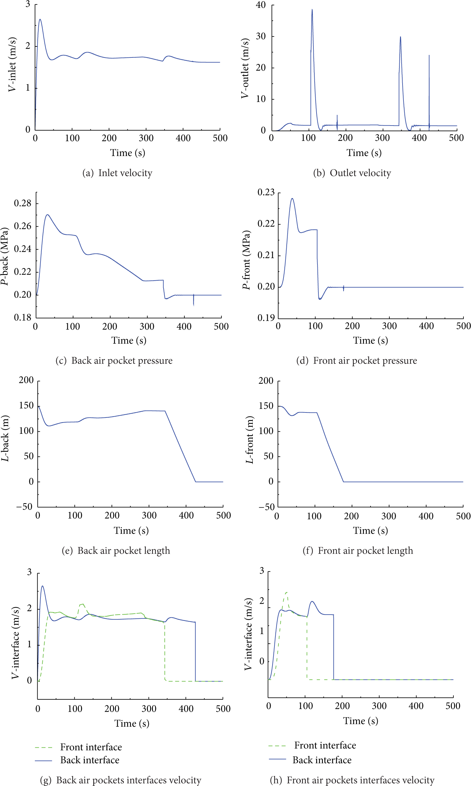
Figure 9 systematically shows the hydraulic characteristics of the whole process from the perspectives of boundary velocity, air pocket pressure, air pocket length (volume), and phase interface velocity, which are analyzed in turn blow.

Figure 9:

Simulation result.

As Figure 9(a) shows, blowing out of the air pockets leads to the small amplitude rise of the inlet velocity which is caused by the decrease of flow friction. When blowing out comes to end, inlet velocity decreases to its normal level. It is noteworthy that, at the beginning of the charge-up process, inlet velocity rises acutely to a high value which is even higher than the moment when blowing out occurs. Subsequently, due to pressure increase of the back air pocket and mass increase of the first liquid segment itself, inlet velocity gradually decreases till reaching equilibrium. This is because that, at the beginning of simulation, inlet pressure increases abruptly from the initial state to the given value, resulting in the abrupt increase of pressure difference on first liquid segment and thus the inlet velocity increases too. Subsequently, this pressure difference is weakened by the movement of the fluid in front of it and pressure of back air pocket even exceeds that of inlet, which slows down the first liquid segment until reaching equilibrium. This shows that, in practical commissioning, pipeline inlet pressure should be carefully controlled to increase slowly to avoid the acute change of inlet velocity.

As Figure 9(b) shows, blowing out process of air pockets can be divided into three phases. (1) Acute phase at high speed: when the front interface of air pocket reaches outlet, the huge pressure difference between air pocket and the atmosphere makes gas blows out at high speed. The outlet velocity suffers acute fluctuation, during which the upmost velocity can reach ten times of the normal value. (2) Stable phase at low speed: after the pressure has been released to the atmosphere level, the outlet velocity returns to normal value. (3) Terminal fluctuation phase: when blowing out comes to end, blowing medium changes abruptly and pipeline outlet returns to the closed state; thus velocity also suffers fluctuation but not that acute as the former.

As Figure 9(c) shows that, at the beginning, velocity of the second liquid slug is lower than that of the first one, which leads to the volume decrease and pressure increase of the back air pocket. Subsequently, as the third liquid slug gradually flows out, resistance applied on the second liquid slug decreases, which makes its velocity continuously rise and exceed that of the first liquid slug, leading to the pressure decrease of the back air pocket. The moment when the first blowing out occurs, pressure of the back air pocket decreases sharply. During the blowing out process of the back air pocket itself, its pressure fluctuates tempestuously. Changing trend of the front air pocket is similar to that of the back one as Figure 9(d) shows.

Figures 9(e) and 9(f) show the changing trend of air pockets length. The most notable phenomenon is that the lengths of both air pockets reach equilibrium before blowing out, which is significant in the influencing factors analysis.

Figures 9(g) and 9(h) show changing trend of the velocity of back and front interfaces of the air pockets. Due to the incompressibility of the liquid, back interface velocity of the back air pocket (as the solid line in Figure 9(g) shows) equals the inlet velocity (as Figure 9(a) shows), front interface velocity of the front air pocket (as the dashed line in Figure 9(h) shows) equals the outlet velocity (as Figure 9(b) shows), and front interface velocity of the back air pocket (as the dashed line in Figure 9(g) shows) equals the back interface velocity of the front air pocket (as the solid line in Figure 9(h) shows). Thus, Figures 9(g) and 9(h) actually show the changing trend of the three liquid slugs.

4.2. Influencing Factors Analysis

In Section 4.1, a typical commissioning charge-up process is simulated and analyzed. Subsequently, several groups of examples are designed to study the influencing factors which are critical to the charge-up process. In engineering practice, what is cared about most is the blowing out process of air pockets; thus the influence from parameters on outlet velocity is focused on.

4.2.1. Influence in the Single Air Pocket Situation

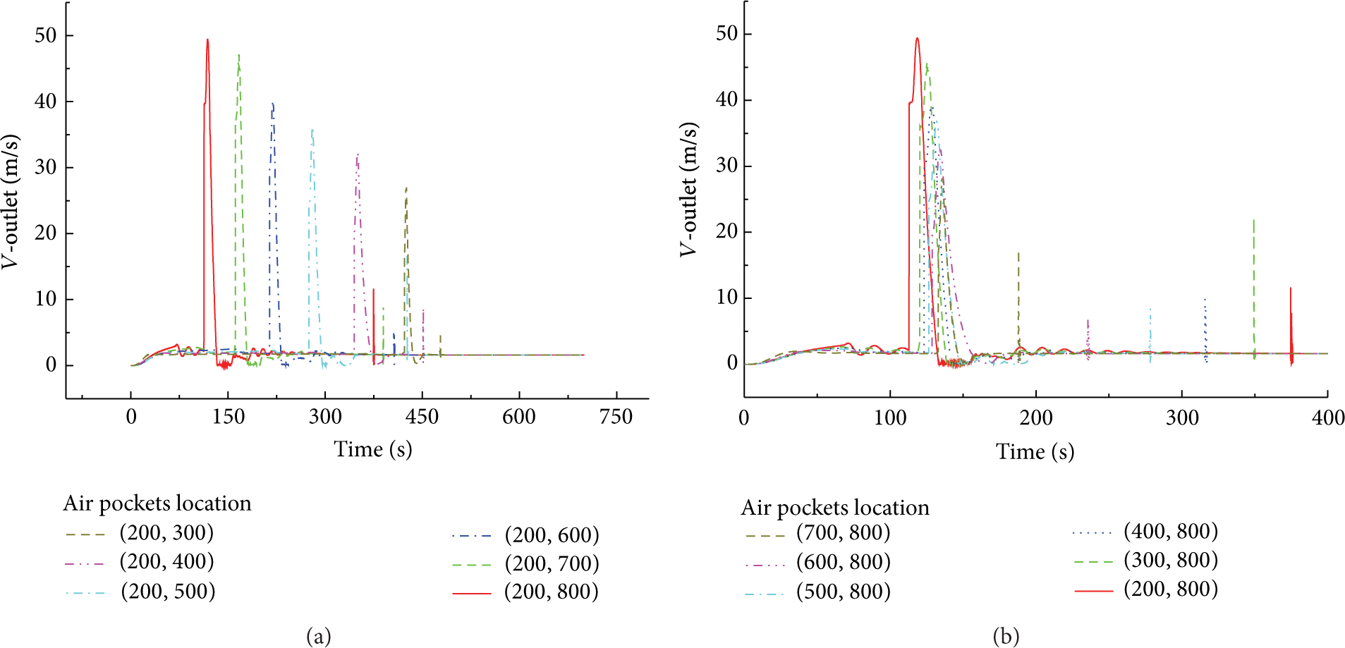
(1) Influence of Initial Location. From Figure 10 we can see that the influence from initial location of air pocket is relatively small. The upmost velocity is almost the same under various initial locations. Only when air pocket is close to the outlet, outlet velocity decreases with the decreasing of distance from air pocket to outlet. From Figures 9(e) and 9(f) we can see that air pocket length endures a process that firstly decreases and then increases until reaching equilibrium. Therefore, as long as the air pocket can reach equilibrium state before blowing out, the outlet velocity is relatively independent of initial location. In the situation that air pocket is close to the outlet in the initial state, it blows out before being fully compressed; thus the upmost velocity is relatively smaller.

Figure 10:

Outlet velocity comparisons of various initial locations.

(2) Influence of Initial Length. When the influence from initial length is studied, this parameter can be changed in two ways: changing the location of front interface or the back one, which this paper studies, respectively. By comparing Figures 11(a) and 11(b) we can see that, in both situations, the longer the initial length is, the more severe the blowing out process would be. This is because the air pocket of longer initial length possesses bigger potential of compressibility and thus can be compressed into higher pressure. Meanwhile, in Figure 11(a), the blowing out moment comes earlier successively with increasing of air pocket initial length, while, in Figure 11(b), the blowing out moment keeps almost invariant with various lengths. From this we can see that air pocket is able to transmit the inlet pressure to outlet. In the parameter range studied, the influence from the gas compressibility of air pocket on its front liquid segment is small and thus the influence on its blowing out moment is small. Therefore, the blowing out moment is largely determined by the distance from its front interface to outlet and is independent of the back interface location.

Figure 11:

(a) Outlet velocity comparisons of various initial lengths (back interface is fixed). (b) Outlet velocity comparisons of various initial lengths (front interface is fixed).

(3) Influence of Diameter. From Figure 12 we can see that the blowing out comes earlier successively with the increasing of diameters. This phenomenon is based on the fact that flow resistance decreases with the increasing of diameter. Thus velocity of the liquid segments increases to make the front interface reach outlet earlier when pipeline diameter increases. However, since the flow velocity of back segment increases due to the same reason, pressure of air pocket would not be compressed into higher pressure, which makes its blowing out process not be more severe.

Figure 12:

Outlet velocity comparisons of various pipeline diameters.

(4) Influence of Pressure Difference. From Figure 13 we can see that the blowing out moment comes earlier successively with the increasing of pressure difference. This is because the velocity of fluid as a whole in pipe increases with the increasing of pressure difference, which makes air pocket reach outlet earlier. When pressure difference is bigger, the back liquid segment would reach higher velocity and that of the front segment increases too, although it has been weakened due to the air pocket. However, the compression degree is still deeper than that of the smaller pressure difference, which makes air pocket reach a higher value and blowing out process more severe. Meanwhile, it is obvious that the bigger the pressure difference is, the higher outlet velocity in equilibrium would be.

Figure 13:

Outlet velocity comparisons of various pressure differences.

(5) Influence of Pipe Length. From Figure 14 we can see that, when initial air pocket length and relative location of air pocket keep invariant, the longer the pipe length is, the less severe the blowing out process would be. The longer the pipe length is, the bigger the fluid mass in pipe would be and the larger flow resistance would be. This makes the velocity of fluid as a whole lower and the compressing effect from liquid segments on air pocket weaker. Thus the blowing out process is less severe.

Figure 14:

Outlet velocity comparisons of various pipe lengths.

4.2.2. Influence in the Two Air Pockets Situation

Influence from several parameters in the situation that single air pocket exists in pipeline on the outlet velocity is analyzed in Section 4.2.1. Next, the situation of two air pockets is analyzed. To avoid redundancy, parameters such as diameter and pipe length are not discussed, while the influence from the interaction between two air pockets on each other is put emphasis on.

(1) Influence from the Existence of Front Air Pocket. From Figure 15 we can see that the existence of front air pocket leads to earlier blowing out moment of back air pocket. This is because the existence of front air pocket is equivalent to the situation that some liquid in front of the air pocket is replaced by gas. On the one hand, flow resistance of gas is smaller than that of liquid and so is its mass, which makes the velocity of fluid in pipeline as a whole increases. On the other hand, the blowing out process makes back air pocket approach outlet earlier.

Figure 15:

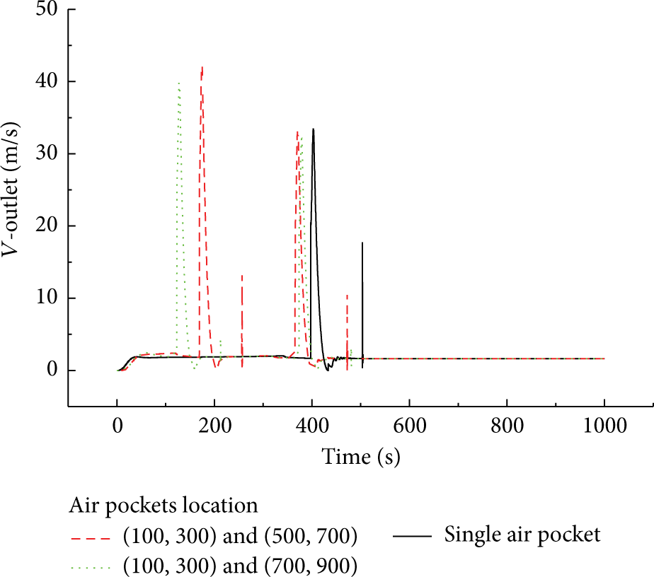
Outlet velocity comparisons of the existence of front air pocket.

(2) Influence of the Front Air Pocket Location. From Figure 16 we can see that the influence from the location of front air pocket is not significant. Combined with the analysis of Section 4.2.1, we know that the influence from front air pocket on back air pocket is by the changing of fluid mass and flow resistance in pipeline, rather than the blowing out process of front air pocket. Due to the fact that blowing out process is usually very short and due to the buffer effect provided by the compressibility of gas, its influence on the blowing out moment of back air pocket is relatively small.

Figure 16:

Outlet velocity comparisons of the initial location of front air pocket.

(3) Influence of the Front Air Pocket Length. As has been discussed in Section 4.2.1 (2), there are two ways to change the air pocket length; the results obtained by them are similar; thus only one is analyzed. As Figure 17 shows, the longer the front air pocket is, the earlier the blowing out moment of back air pocket would be. This is because the longer the front air pocket is, the bigger total mass of the fluid in pipeline would be and the smaller flow resistance would be, which makes the back air pocket approach outlet faster.

Figure 17:

Outlet velocity comparisons of the initial length of front air pocket.

(4) Influence of the Existence of Back Air Pocket. As Figure 18 shows, although the existence of back air pocket makes the velocity of the fluid back of the front air pocket increase, the blowing out moment of front air pocket almost keeps invariant because of the buffer effect provided by the compressibility of gas. Meanwhile, due to the increasing of the velocity of the fluid back of the front air pocket, the front air pocket is compressed into a deeper degree, which makes its blowing out process more severe.

Figure 18:

Outlet velocity comparisons of the existence of back air pocket.

(5) Influence of the Back Air Pocket Location. As Figure 19 shows, influence from the location of the back air pocket on the blowing out process is not significant. As has been discussed in Section 4.2.1, as long as the length of the air pocket reaches equilibrium before blowing out, its initial location has little influence on the outlet velocity. Within the variation range of parameters in this set of examples, the initial location of the back air pocket hardly influences the equilibrium of both front and back air pockets. This leads to the similarity of the blowing out process among this set of examples.

Figure 19:

Outlet velocity comparisons of the initial location of back air pocket.

(6) Influence of the Back Air Pocket Length. As Figure 20 shows, influence from the length of back air pocket on the blowing out process of front air pocket is small. This is because the influence from the gas compressibility of the back air pocket on its front liquid segment is negligible in the parameter range, and thus the influence on the blowing out process of the front air pocket is small. Meanwhile, the longer the back air pocket is, the more severe the blowing out process of back air pocket itself would be, resulting from their gradually deeper compression degree.

Figure 20:

Outlet velocity comparisons of the initial length of back air pocket.

5. Conclusions

In this paper, commissioning charge-up process of horizontal pipeline with entrapped air is simulated. Velocity and pressure of the whole line are obtained and analyzed. On the base of this, influence of the initial location and length of the air pocket on the whole charge-up process is studied. Following conclusions are drawn.

In the typical commissioning situation in which inlet pressure is constant, inlet velocity first acutely rises and then gradually decreases till reaching steady.

Blowing out process of the air pockets can be divided into three phases: acute phase at high speed, stable phase at low speed, and terminal fluctuation phase. The acute change of outlet velocity propagates along the pipeline to the upstream and leads to a small amplitude velocity increase of the whole line. At the beginning and end of the blowing out, flow parameters of the outlet suffer acute fluctuation.

Several factors, such as initial length of air pockets, pressure difference between inlet and outlet, and pipeline length, have notable influence on the blowing out process, while the influence from initial location of air pockets and pipeline diameter is relatively small.

Entrapped air pockets cause seriously unsteady operation condition of the whole pipeline when they blow out, which may result in accident in the commissioning process. Thus, it is necessary to take proper measures, such as exhaustion, to prevent the formation of the air pockets in the pipeline.

These conclusions are based on the idealized model which contains simplified conditions and a certain gap is inevitable between the model and the actual engineering reality. Thus further researches need to be improved in the future.

Conflict of Interests

The authors declare that there is no conflict of interests regarding the publication of this paper.

Footnotes

Acknowledgment

The study was supported by the National Science Foundation of China (nos. 51325603 and 51276198).

References

Zhang

and Vairavamoorthy

, “Transient flow in rapidly filling air-entrapped pipelines with moving boundaries,” Tsinghua Science and Technology, vol. 11, no. 3, pp. 313–323, 2006.

Zhang

and Vairavamoorthy

, “Application of method-of-lines to charging-up process in pipelines with entrapped air,” Tsinghua Science and Technology, vol. 11, no. 3, pp. 324–331, 2006.

Jiang

S.-J.

, and Bao

, “Modeling and analyzing of low pressure pipeline transients accompanying gas bubbles and cavitation,” Journal of Aerospace Power, vol. 22, no. 12, pp. 2062–2067, 2007.

Liu

D.-Y.

and Suo

L.-S.

, “Rigid model for transient flow in pressurized pipe system containing trapped air mass,” Advances in Water Science, vol. 15, no. 6, p. 717, 2004.

Yang

, and Zheng

, “Numerical simulation of water-filling process in pressure conduit,” Journal of Hydraulic Engineering, vol. 38, no. 2, pp. 171–175, 2007.