A Novel Separable Model and Decomposition Method for Sensor Locational Decision Problem

Abstract

This paper proposes a new separable model for the sensor locational decision problem covering a line (SLDPCL). By decomposing a multivariate function into several univariate functions, a separable outer approximation methodology that can be used to improve the outer approximation of classical convex programming technique is presented. A novel outer approximation method (OAM) for this proposed separable model is proposed. The algorithm alternates between solving a mixed integer linear program and a convex nonlinear program (NLP). An improved interior point method based on optimal centering parameter is employed to solve the NLP subproblem. The simulation results for test instances that range in size from 10 to 20000 sensors show that the proposed method is fast and robust, and the method is very promising for large-scale SLDPCL problems due to its excellent scalability.

1. Introduction

Sensor locational decision problem covering a line (SLDPCL) is a problem to find a subset covering a given length segment at minimum cost with giving a set of sensors. And these sensors have variable radii with costs depending on their radii and fixed costs [1]. This problem was motivated by the following application. There is a river in a city, over which we need to track possible activities of objects or people. For this purpose, we need to locate a set of sensors so that every point on the river is under supervision by at least one sensor. It is assumed that (i) the river can be modeled as a tree network consisting of line segments and (ii) each sensor has a field of view defined by a radius. It is reasonable to view the river as piecewise strips of finite lengths. Then we may focus on the problem for a strip. The above problem for a strip can be viewed as an SLDPCL. Although the problem is easily stated, the actual locational decision is complicated due to some additional factors. Coverage depends not only on the river topology, sensor type, and power, but also on several parameters such as width of river and obstacles over it, potentially forbidden areas where sensors may not be located, and other characteristics associated with the physical environment, for example, the atmospheric and water conditions. Readers can further refer to [2] for further details on this scenario.

In this paper, a new separable mixed integer nonlinear programming (MINLP) formulation for the SLDPCL problem by decomposing the multivariate function into several univariate functions is presented. The outer approximation of a decomposed equivalent is tighter than the direct outer approximation of the original multivariate problem, so a tighter separable outer approximation methodology is proposed to improve the existing outer approximation method (OAM). Then, an improved OAM is proposed to solve the separable formulation for SLDPCL problem. This novel method consists of solving an alternating sequence of a nonlinear programming (NLP) problem and a mixed integer linear programming (MILP) problem. In order to solve the NLP problems efficiently, a new quickly interior point algorithm was presented based on the techniques of optimal centering parameter (OCP) and multiple centrality correction (MCC). At last, the novel OAM integrating improved interior point method (IPM) is presented to solve this separable model for SLDPCL problem. Ten to 20000 sensors instances have been solved by the proposed method, and the results show that the method is scalable for large-scale SLDPCL problem. The main contributions of this paper are as follows.

• (i)

By simply introducing an auxiliary variable, we move the nonlinear function from objective function to constraints for the classic MINLP formulation of SLDPCL problem. After letting equivalent several univariate functions substitute for a multivariate function, we obtain a new separated formulation for SLDPCL problem.

(ii)

An improved OAM is presented to solve the SLDPCL problem based on the aforementioned separated formulation. The proposed method can obtain tighter MILP relaxation than the traditional OAM does. Solving infeasible subproblem is not needed for the improved method, because all feasible solutions of the MILP relaxations are feasible for the corresponding SLDPCL problem as well.

(iii)

A new quickly interior point algorithm was presented for solving NLP subproblems based on the techniques of OCP and MCC. Named as I-IPM, the proposed method involves integrating equilibrium distance-quality function (ED-QF) to establish a mathematical model for evaluating centering parameter. And the approximate expression of this model, which can be solved with fewer computations than the original one, was proposed using the linearization technique. After solving the approximate model with the line search technique, the optimal centering parameters can be obtained for the proposed method to own longer step length and less number of iterations than other IPMs. The aim of using MCC is twofold: (a) to increase the step length in both primal and dual spaces and (b) to offer better convergence performances.

The rest of this paper is organized as follows. Section 2 introduces some related works in coverage of sensor networks, especially in SLDPCL. Section 3 describes the classic MINLP formulation of SLDPCL, and we present a separable formulation for SLDPCL based on the classic one in this section as well. In Section 4, we present the improved OAM to solve the separable formulation, which consists of solving an alternating sequence of NLP and MILP. In Section 5, we present an improved IPM to solve those NLP subproblems effectively. Simulations are conducted and the results are shown in Section 6. Finally, we conclude this paper and point out the future work in Section 7.

2. Related Works

There are many applications of SLDPCL. In [6], with the assumptions that (i) a set of potential resources; (ii) a fixed activation cost for each resource; (iii) the congestion heavily influences the cost of a resource, a single-commodity network flow problem can be formulated and solved by using SLDPCL model. The effect of introducing additional stops in the existing railway network can be formulated as an SLDPCL model as well. This problem is comprised of covering a set of points in the plane by sensors. And the centers of these sensors have to lie on a set of line segments that represents the railway [7]. If only one period is considered, the unit commitment problem in power system also can be formulated as an SLDPCL model [8].

SLDPCL is a special case of coverage in sensor networks. Coverage, which reflects how well a sensor field is monitored, is one of the most important performance metrics to measure sensor networks. Simply said, sensor coverage models are abstract models trying to quantify how well sensors can sense physical phenomena at some location, or, in other words, how well sensors can cover such locations. In sensor networks, coverage problems can arise in all network stages and can be formulated in various ways with different scenarios, assumptions, and objectives [9]. There are two important problems relating to coverage. The first one is to formulate mathematical model. The other one is to solve the large-scale coverage problem models efficiently.

2.1. Modeling Coverage Problems

Sensor coverage models measure the sensing capability and quality by capturing the geometric relation between a space point and sensors. Modeling coverage problems fall into the field of geometric covering, in which some points or some areas are required to be covered by geometric objects [10]. For example, Chvátal [11] introduces the art gallery problem, in which cameras are to be placed to watch every wall of an art gallery room. The room is assumed to be a polygon with n sides and h holes, and the cameras are assumed to have a viewpoint of 360° and rotate at an infinite speed. It is proved that at most $\lfloor (n+h)/\mathrm{3}\rfloor$ cameras are sufficient. In [12], Huang and Tseng study the problem of deciding whether an area is sufficiently covered, in the sense that every point in the area is covered by at least k sensors. They prove that as long as the perimeters of the sensors are sufficiently covered, the whole area is sufficiently covered. In [13], Wang et al. study the relationship between coverage and connectivity. They prove that if a region is k-covered then the sensor network is k-connected as long as the communication range is at least twice of the sensing range. In [1], the problem of coverage in a line segment is formulated as mixed integer nonlinear programming (MINLP) with quadratic objective function and linear constraints. Reference [14] shows that solving the aforementioned coverage problem with MINLP is NP-hard problem.

2.2. Solving Methods

The coverage problem often can be formulated as MINLP. As pointed in [14], this MINLP is NP-hard problem, which is rather difficult to solve efficiently for large-scale instances. For the problem in which a set of m fixed locations for radars and a set of n locations for the points are given, all located along a fixed line, [15] gives an $O({(n+m)}^{\mathrm{3}})$ dynamic programming approach. To lower the time complexity, [15] gives a linear-time 4-approximation algorithm as well. Reference [16] shows that the line segment coverage problem is polynomial time solvable by reducing it to an integer linear program with totally unimodular matrix. All these methods are based on heuristics or approximations, which cannot guarantee obtaining the global optimal solutions. In [17], Li et al. consider the problem of covering a line segment with wireless sensors of adjustable ranges. They present a polynomial time exact algorithm for the discrete case. However, for the continuous case, where the cost of each sensor is given by a function $f(r)=r^{\alpha }$ , the polynomial-time algorithm presented by them is an approximated one. Reference [18] presents an $O(n^9)$ dynamic programming algorithm for the radar placement and power assignment problem, where n is the number of crucial points to be monitored. However, the proposed method often suffers from the curse of dimensionality just the same as classic dynamic programming does.

SLDPCL can be formulated as MINLP too, but it has some characteristics: (i) the need to cover a single line segment and (ii) a fixed activation cost for each sensor. According to these characteristics, searching more effective algorithm to solve SLDPCL is necessary. In [1], the authors provide an exact solution algorithm, based on a Lagrangian relaxation and a subgradient algorithm, to find a lower bound for SLDPCL. But the feasible solution only can be obtained by using a heuristic method. In [19], an $O(n\log n)$ time 12-factor approximation algorithm is proposed for the problem of covering a set of line segments with minimum number of sensors. However, the algorithm needs that the line segments are axis-parallel. In [3], the bound of SLDPCL model is improved by using the convex envelope of the single block of the objective function. Then the MINLP model of SLDPCL is reformulated as mixed integer second-order cone programming (MISOCP), which can be solved by general-purpose mixed integer programming solvers. However, [20] points out that directly passing MISOCP to the solvers is less competitive than using piecewise linear approximations.

In the last 40 years, some algorithms have been proposed for solving convex MINLP to optimality [21]. In the early 70s, Geoffrion generalized Benders decomposition (BD) to make an exact algorithm for convex MINLP [21]. And in the 80s, Duran and Grossmann introduced the OAM [22]. Both BD method and OAM are decomposition strategies, which can solve MINLP efficiently. However, BD method and its variants use the dual information for outer approximation, while the OAM method and its variants are based on the use of the optimal primal information. So far, BD method has been used to solve the location problem successfully [23], which decomposes the location problem into a master problem that is an integer optimization problem and an NLP subproblem. However, to the authors’ knowledge, up to now, OAM method has not been used for solving location problem.

Solving the NLP subproblems efficiently plays a pivotal role in solving MINLP model for SLDPCL problem by using OAM method. IPMs [5] are currently considered the most powerful algorithms for large-scale NLPs. Some of the key ideas, such as primal-dual steps and center parameter, carry over directly from the LP case [4], but several important new challenges arise [24]. These include the strategy for updating the barrier parameter and the need to ensure progress toward the solution according to the structure of application problems.

3. Separable MINLP Formulation for SLDPCL

The traditional MINLP formulation of SLDPCL is reported in [1] by Agnetis et al. In this section, we give a separable MINLP for SLDPCL, which can be solved more efficiently by using decomposition strategies, especially by using OAM.

Suppose that there are q available discs (sensors), and they are represented by the set $Q=\{\mathrm{1,2},\dots ,q\}$ . For all $i\in Q$ , at most one copy of disc i may be used for covering the line segment and the power level is allowed as $0\le r_i\le {\stackrel{-}{r}}_i$ , where $r_i$ denotes the disc coverage diameter and ${\stackrel{-}{r}}_i$ denotes the cover limit for sensor i. The assumption may appear restrictive for real applications, but note that usage of multiple copies of the same disc type may be modeled by including in Q a suitable number of items with the same characteristics.

For any selected disc $i\in Q$ , its contribution in the total cost function is

$$\begin{array}{cc}& {c_{f,}}_i\left(r_i\right)=\{\begin{array}{cc}\mathrm{0}\hfill & \text{if}\hspace{0.17em}\hspace{0.17em}{r}_i=\mathrm{0}\hfill \\ {\alpha }_i+g_i\left(r_i\right)\hfill & \text{if}\hspace{0.17em}\hspace{0.17em}{r}_i>\mathrm{0},\hfill \end{array}\end{array}$$

(1)

where the setup cost ${\alpha }_i>\mathrm{0}$ and operational cost $g_i(r_i)={\beta }_i{r}_i+{\gamma }_i(r_i{)}^{\mathrm{2}},\hspace{0.17em}{\beta }_i\ge \mathrm{0},\hspace{0.17em}{\gamma }_i>\mathrm{0}$ .

The objective function of the SLDPCL problem, representing the total cost to be minimized, has the form

$$\begin{array}{cc}& \min {\displaystyle \sum }_{i\in Q}({\alpha }_i{u}_i+{\beta }_i{r}_i+{\gamma }_i{\left(r_i\right)}^{\mathrm{2}}),\end{array}$$

(2)

where $u_i$ indicate selected sensors $i\in Q$ :

$$\begin{array}{cc}& u_i=\{\begin{array}{cc}1\hfill & \text{sensor}\hspace{0.17em}\hspace{0.17em}i\hspace{0.17em}\hspace{0.17em}\text{has}\hspace{0.17em}\hspace{0.17em}\text{been}\hspace{0.17em}\hspace{0.17em}\text{sellected}\hfill \\ 0\hfill & \text{sensor}\hspace{0.17em}\hspace{0.17em}i\hspace{0.17em}\hspace{0.17em}\text{has}\hspace{0.17em}\hspace{0.17em}\text{not}\hspace{0.17em}\hspace{0.17em}\text{been}\hspace{0.17em}\hspace{0.17em}\text{sellected}.\hfill \end{array}\end{array}$$

(3)

The constraints of the SLDPCL problem are as follows.

• (1)

Covering constraint is

$$\begin{array}{cc}& {\displaystyle \sum }_{i\in Q}{r}_i-r_{\text{all}}=\mathrm{0},\end{array}$$

(4)

where $r_{\text{all}}$ denotes the length of line segment needing to be covered.

• (2)

  Sensor coverage distance limits are

  $$\begin{array}{cc}& \mathrm{0}\le r_i\le u_i{\stackrel{-}{r}}_i.\end{array}$$

  (5)

Constraints (5) force $r_i$ to be zero when the corresponding sensor i is not selected (and therefore the corresponding cost contribution is zero). Constraint (4) is the coverage constraint that assures that the whole line segment is covered.

Equations (4)-(5) are linear constraints. These constraints can be abbreviated as $A_u\mathit{u}+A_x\mathit{r}\le {\mathit{a}}_{ux}$ for the sake of convenience, where $\mathit{u}=(u_i)$ , $\mathit{r}=(r_i)$ , $\hspace{0.17em}i=1,\dots ,q$ , $A_u,A_x$ are the coefficient matrices and ${\mathit{a}}_{ux}$ is the constant vector.

Consequently, the SLDPCL problem is conveniently formulated as the following MINLP:

$$\begin{array}{l}\min \hspace{1em}{\displaystyle \sum }_{i\in Q}({\alpha }_i{u}_i+{\beta }_i{r}_i)+g\left(\mathit{r}\right)\mathrm{\hspace{0.17em}\hspace{0.17em}}\\ \text{s}.\text{t}.\mathrm{\hspace{0.17em}\hspace{0.17em}}\hspace{1em}\{\begin{array}{ll}{A}_u\mathit{u}+A_x\mathit{r}\le {\mathit{a}}_{ux}\mathrm{\hspace{0.17em}\hspace{0.17em}}\mathrm{\hspace{0.17em}\hspace{0.17em}}\hfill & \hfill \\ \mathit{u}\in {\left\{\mathrm{0,1}\right\}}^q,\hfill & \hfill \end{array}\end{array}$$

(6)

where $g(\mathit{r})={\sum }_{i=1}^q{\gamma }_i(r_i{)}^2$ . By introducing an auxiliary variable η, the SLDPCL problem (6) is equivalent to the form denoted as SMIP:

$$\begin{array}{l}\min \hspace{1em}{\displaystyle \sum }_{i\in Q}({\alpha }_i{u}_i+{\beta }_i{r}_i)+\eta \mathrm{\hspace{0.17em}\hspace{0.17em}}\\ \text{s}.\text{t}.\mathrm{\hspace{0.17em}\hspace{0.17em}}\hspace{1em}\{\begin{array}{ll}g\left(\mathit{r}\right)\le \eta \hfill & \hfill \\ A_u\mathit{u}+A_x\mathit{r}\le {\mathit{a}}_{ux}\hfill & \hfill \\ \mathit{u}\in {\left\{\mathrm{0,1}\right\}}^q.\hfill & \hfill \end{array}\end{array}$$

(7)

Problem (7) is special MINLP with separable constraint $g(\mathit{r})\le \eta$ . In the following sections, we will discuss how to solve this separable model for SLDPCL problem more efficiently. Model (7) is convex MINLP because of the following.

• (a)

$g(\mathit{r})\le \eta$ is convex constraint due to $a_i>0$ for $\forall i\in Q$ .

(b)

The other constraints and the object function all are linear.

4. OAM for Separable Mixed Integer Programming of SLDPCL

The OAM, a very successful approach to solving convex MINLP, was first developed by Duran and Grossmann [22] and then subsequently extended to a general mixed integer convex programming, nonconvex MINLP, and separable MINLP [25]. The OAM consists of solving an alternating sequence of a primal problem and MILP. A sequence of valid nondecreasing lower bounds and nonincreasing upper bounds is generated by the OAM which converges in a finite number of iterations.

In this section, we consider the solution of the SMIP formulation (7) for SLDPCL problem. The function g is convex and separable. By separable, we mean that the function g can be rewritten as a sum of some convex univariate functions [25]; that is, $g(\mathit{r})={\sum }_{i\in Q}{g}_i(r_i)$ , where $g_i={\gamma }_i(r_i{)}^2$ is convex univariate function. Now, we describe OAM algorithms [25] to solve the SLDPCL model SMIP.

The OAM solves SMIP formulation (7) by alternating finitely between an NLP subproblem and an MILP relaxed master problem. And this master problem is obtained by replacing the nonlinear constraints with their linear outer approximations taken in a set of points $\mathrm{\Omega }=\{{\widehat{\mathit{r}}}^1,\dots ,{\widehat{\mathit{r}}}^{n_{\mathrm{\Omega }}}\}$ . The corresponding outer approximation master MILP of SMIP can be formed as

$$\mathrm{MILP}(\mathrm{\Omega })\begin{array}{l}\min \hspace{1em}{\displaystyle \sum }_{i\in Q}\left({\alpha }_i{u}_i+{\beta }_i{r}_i\right)+\eta \mathrm{\hspace{0.17em}\hspace{0.17em}}\\ \text{s}.\text{t}.\mathrm{\hspace{0.17em}\hspace{0.17em}}\hspace{1em}\{\begin{array}{ll}g\left({\widehat{\mathit{r}}}^s\right)+\nabla g{\left({\widehat{\mathit{r}}}^s\right)}^T\left(\mathit{r}-{\widehat{\mathit{r}}}^s\right)\le \eta ,\hfill & \hfill \\ \hspace{1em}\hspace{1em}\hspace{1em}\hspace{1em}\hspace{1em}\hspace{1em}\hspace{0.5em}s=\mathrm{1},\dots ,n_{\mathrm{\Omega }}\hfill & \hfill \\ A_u\mathit{u}+A_x\mathit{r}\le {\mathit{a}}_{ux}\hfill & \hfill \\ \phantom{\mathit{l}\mathit{l}\mathit{l}\mathit{l}\mathit{l}\mathit{l}\mathit{l}\mathit{l}\mathit{l}}\mathit{u}\in {\left\{\mathrm{0,1}\right\}}^q.\hfill & \hfill \end{array}\end{array}$$

(8)

The integer vector ${\mathit{u}}^{k+1}$ obtained by MILP( $\mathrm{\Omega }$ ) is feasible for SMIP (7). The main theoretical justification of OAM is that it has the same optimal value as SMIP if MILP ( $\mathrm{\Omega }$ ) contains a suitable set of linearization points. Next, the NLP subproblem for fixed value of the integer decision vector ${\mathit{u}}^{k+1}$ is defined as

$$\mathrm{NLP}({\mathbf{u}}^{k+1})\begin{array}{l}\min \hspace{1em}{\displaystyle \sum }_{i\in Q}\left({\alpha }_i{u}_i+{\beta }_i{r}_i\right)+\eta \mathrm{\hspace{0.17em}\hspace{0.17em}}\\ \text{s}.\text{t}.\mathrm{\hspace{0.17em}\hspace{0.17em}}\hspace{1em}\{\begin{array}{ll}g\left(\mathit{r}\right)\le \eta \mathrm{\hspace{0.17em}\hspace{0.17em}}\hfill & \hfill \\ A_u{\mathit{u}}^{k+\mathrm{1}}+A_x\mathit{r}\le {\mathit{a}}_{ux}.\hfill & \hfill \end{array}\end{array}$$

(9)

We are now in a position to give the outer approximation algorithm in full detail [25].

Algorithm OAM

Initialization. Set the superbound $z_{\text{up}}=10^{10}$ and lower bound $z_{\text{low}}=10^{-10}$ ; set the tolerance ε.

Step 1.

Solve the continuous relaxation of (7) with IPM; the optimal solution is ${\mathit{y}}^0=({\mathit{u}}^0,{\mathit{r}}^0,{\eta }^0)$ and $k=1$ .

Do while $(z_{\text{up}}-z_{\text{low}})/(z_{\text{up}}+z_{\text{low}})>\epsilon$  

Step 2.

Construct MILP (8), and solve it with branch-cut method. The optimal solution of (8) is $({\mathit{u}}^{k+1},\stackrel{-}{\mathit{r}},\stackrel{-}{\eta })$ , and optimal value is $z_{\text{low}}$ .

Step 3.

Construct NLP (9), and solve it with IPM. The optimal solution of (9) is $({\mathit{r}}^{k+\mathrm{1}},{\eta }^{k+\mathrm{1}})$ . If   ${\sum }_{i\in Q}({\alpha }_i{u}_i^{k+\mathrm{1}}+{\beta }_i{r}_i^{k+\mathrm{1}})+{\eta }^{k+\mathrm{1}}\mathrm{\hspace{0.17em}\hspace{0.17em}}<z_{\text{up}}$ , let $z_{\text{up}}={\sum }_{i\in Q}({\alpha }_i{u}_i^{k+\mathrm{1}}+{\beta }_i{r}_i^{k+\mathrm{1}})+{\eta }^{k+\mathrm{1}}\mathrm{\hspace{0.17em}\hspace{0.17em}}$ , and we get the current solution and object value are $({\mathit{r}}^{k+\mathrm{1}},{\mathit{u}}^{k+\mathrm{1}})$ and $z_{\text{up}}$ separately.

Step 4.

$k=k+\mathrm{1}$ ; update $\mathrm{\Omega }=\mathrm{\Omega }\cup \{{\mathit{r}}^{k+\mathrm{1}}\}$ .

End do

Step 5.

Output optimal object value $z_{\text{up}}$ and the optimal solution $({\mathit{r}}^{k+1},{\mathit{u}}^{k+1})$ .

The convex function g can be outer approximated by subgradient inequalities through a single-step procedure that yields MILP ( $\mathrm{\Omega }$ ). Furthermore, it can be several-step approximated by constructing subgradient inequalities for some univariate functions $g_i,i=1,\dots ,q$ .

First, based on the analysis above, in (7), we introduce an auxiliary variable ${\upsilon }_i$ for each univariate function $g_i$ , and the SLDPCL problem (7) can be reformulated as the separated model of the form

$$\begin{array}{l}\min \hspace{1em}{\displaystyle \sum }_{i\in Q}({\alpha }_i{u}_i+{\beta }_i{r}_i)+\eta \mathrm{\hspace{0.17em}\hspace{0.17em}}\\ \text{s}.\text{t}.\mathrm{\hspace{0.17em}\hspace{0.17em}}\hspace{1em}\{\begin{array}{ll}{\displaystyle \sum }_{i=\mathrm{1}}^q{\upsilon }_i\le \eta \hfill & \hfill \\ g_i\left(r_i\right)={\gamma }_i{\left(r_i\right)}^{\mathrm{2}}\le {\upsilon }_i,\hspace{1em}\mathrm{\hspace{0.17em}\hspace{0.17em}}i=\mathrm{1},\dots ,q\hfill & \hfill \\ A_u\mathit{u}+A_x\mathit{r}\le {\mathit{a}}_{ux}\hspace{1em}\hspace{1em}\mathit{u}\in {\left\{\mathrm{0,1}\right\}}^q.\hfill & \hfill \end{array}\end{array}$$

(10)

Clearly, if $(z,\upsilon ),\hspace{0.17em}z=(\mathit{u},\mathit{r},\eta )$ , $\upsilon =({\upsilon }_i)$ , is an optimal solution of (10), then z is optimal for (7). According to [25], we have the following theorem.

Theorem 1.

Give points ${\mathit{r}}^s,s=1,\dots ,n_{\mathrm{\Omega }}$ . Let $S_1=\{(\mathrm{\Gamma },\mathit{r})\mid \mathrm{\Gamma }\ge g({\mathit{r}}^s)+\nabla g({\mathit{r}}^s)(\mathit{r}-{\mathit{r}}^s),s=1,\dots ,n_{\mathrm{\Omega }}\}$ and $S_2=\{(\mathrm{\Gamma },\mathit{r})\mid \mathrm{\Gamma }\ge {\sum }_{j=1}^q{\upsilon }_j,{\upsilon }_j\ge g_j(r_j^s)+\nabla g_j(r_j^s)(r_j-r_j^s),s=1,\dots ,n_{\mathrm{\Omega }},j\in Q\}$ . Then, $S_{\mathrm{1}}\supseteq S_{\mathrm{2}}$ .

It is easy to observe from Theorem 1 that the linear outer approximation MILP of (10) may be tighter than the one of (7). More precisely, Theorem 1 shows that, to obtain a linear relaxation of (7) of the same strength as a linear approximation of (10), one needs exponentially many linearization points. Thus, in general, we can expect the extended formulation to perform much better than the initial one in an outer approximation algorithm. Then, a tighter outer approximation master MILP for SMIP is given by

$$T\text{-}MILP\hspace{0.17em}(\mathrm{\Omega })\begin{array}{l}\min \hspace{1em}{\displaystyle \sum }_{i\in Q}({\alpha }_i{u}_i+{\beta }_i{r}_i)+\eta \mathrm{\hspace{0.17em}\hspace{0.17em}}\\ s.t\hspace{1em}\{\begin{array}{ll}{\displaystyle \sum }_{i=\mathrm{1}}^q{\upsilon }_i\le \eta \hfill & \hfill \\ g_i\left({{\widehat{r}}_i}^s\right)+g_i^{\prime }\left({{\widehat{r}}_i}^s\right)\left(r_i-{{\widehat{r}}_i}^s\right)\le {\upsilon }_i,\hfill & \hfill \\ \hspace{1em}i=\mathrm{1},\dots ,q,\mathrm{\hspace{0.17em}\hspace{0.17em}}\mathrm{\hspace{0.17em}\hspace{0.17em}}s=\mathrm{1},\dots ,n_{\mathrm{\Omega }}\hfill & \hfill \\ A_u\mathit{u}+A_x\mathit{r}\le {\mathit{a}}_{ux},\hspace{1em}\mathit{u}\in {\left\{\mathrm{0,1}\right\}}^q.\hfill & \hfill \end{array}\end{array}$$

(11)

We want to note that the T-MILP( $\mathrm{\Omega }$ ) (11) is a lower linear approximation for MINLP model (10) of SLDPCL problem. We cannot guarantee that the solutions of T-MILP are feasible for MINLP (10). In [25], an inner approximation, which is MILP, is solved to obtain feasible solutions of (10). In our method, the T-MILP model has included all the constraints of SLDPCL problem. So the solutions of (11) are feasible for SLDPCL problem.

In addition, according to the description of Algorithm OAM in this section, we know that there are two NLPs, (9) in Step 3 and the relaxation of (7) in Step 1, which need to be solved efficiently. IPM [5] is a very appealing approach to large-scale NLP. We present a new quickly interior point algorithm for solving these two NLPs based on the techniques of OCP and MCC in the following section.

5. Improved IPM for NLP

5.1. Primal-Dual IPM

IPMs became quite popular after 1984, when N. Karmarkar announced a fast polynomial-time interior method for linear programming [5]. In this subsection, we introduce classic primal-dual IPM and analyze the difficulty of setting centering parameter in IPM. Then, our improvement in setting centering parameter is proposed in the following subsections.

Without losing the generalization, we consider the NLP writing in a formal style as follows

$$\begin{array}{l}\min \hspace{1em}f\left(\mathit{x}\right)\\ \text{s}.\text{t}.\hspace{1em}\{\begin{array}{ll}\mathit{h}\left(\mathit{x}\right)=\mathrm{0}\hfill & \hfill \\ \underset{\_}{\mathit{g}}\le \mathit{g}\left(\mathit{x}\right)\le \stackrel{-}{\mathit{g}}.\hfill & \hfill \end{array}\end{array}$$

(12)

By introducing slack variables in the inequality of constraints and introducing logarithmic barrier penalty terms in the objective function, we obtain the following logarithmic barrier problem for (12):

$$\begin{array}{l}\min \hspace{1em}\phi =f\left(\mathit{x}\right)-\mu {\displaystyle \sum }_{j=\mathrm{1}}^r\ln l_j-\mu {\displaystyle \sum }_{j=\mathrm{1}}^r\ln u_j\\ \text{s}.\text{t}.\hspace{1em}\{\begin{array}{ll}\mathit{h}\left(\mathit{x}\right)=\mathrm{0}\hfill & \hfill \\ \mathit{g}\left(\mathit{x}\right)-\mathit{l}-\underset{\_}{\mathit{g}}=\mathrm{0}\hfill & \hfill \\ \mathit{g}\left(\mathit{x}\right)+\mathit{u}-\stackrel{-}{\mathit{g}}=\mathrm{0}.\hfill & \hfill \end{array}\end{array}$$

(13)

The Lagrangian function of (13) is

$$\begin{array}{l}L\left(\mathit{X},\mu \right)=f\left(\mathit{x}\right)-y^T\mathit{h}\left(\mathit{x}\right)\\ -{\mathit{z}}^T\left(\mathit{g}\left(\mathit{x}\right)-\mathit{l}-\underset{\_}{\mathit{g}}\right)-\mu {\displaystyle \sum }_{j=\mathrm{1}}^r\ln l_j\\ -{\mathit{w}}^T\left(\mathit{g}\left(\mathit{x}\right)+\mathit{u}-\stackrel{-}{\mathit{g}}\right)-\mu {\displaystyle \sum }_{j=\mathrm{1}}^r\ln u_j.\end{array}$$

(14)

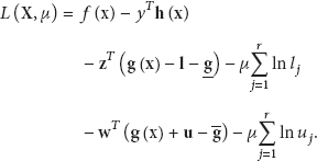
According to the gradients of the Lagrangian function with respect to variables $\mathit{x}$ , multipliers $\mathit{y}$ , $\mathit{z}$ , $\mathit{w}$ , and slack variables $\mathit{l}$ , $\mathit{u}$ , we obtain the perturbing KKT equation of (12),

$$\begin{array}{l}\mathit{K}\left(\mathit{X},\mu \right)\\ \hspace{1em}=[L_{\mathit{x}}\left(\mathit{X}\right);L_{\mathit{y}}\left(\mathit{X}\right);L_{\mathit{z}}\left(\mathit{X}\right);\\ L_{\mathit{w}}\left(\mathit{X}\right);L_{\mathit{l}}\left(\mathit{X},\mu \right);L_{\mathit{u}}\left(\mathit{X},\mu \right)\phantom{L_{\mathit{x}}\left(\mathit{X}\right);L_{\mathit{y}}\left(\mathit{X}\right);L_{\mathit{z}}\left(\mathit{X}\right)}]=\mathrm{0}\end{array}$$

(15)

$$\begin{array}{l}\hspace{0.17em}{L}_{\mathit{x}}\left(\mathit{X}\right)=-\nabla f\left(\mathit{x}\right)+\nabla \mathit{h}\left(\mathit{x}\right)\mathit{y}+\nabla \mathit{g}\left(\mathit{x}\right)(\mathit{z}+\mathit{w})\end{array}$$

(16)

$$\begin{array}{l}\hspace{0.17em}{L}_{\mathit{y}}\left(\mathit{X}\right)=\mathit{h}\left(\mathit{x}\right)\\ \hspace{0.17em}{L}_{\mathit{z}}\left(\mathit{X}\right)=\mathit{g}\left(\mathit{x}\right)-\mathit{l}-\underset{\_}{\mathit{g}}\\ \hspace{0.17em}{L}_{\mathit{w}}\left(\mathit{X}\right)=\mathit{g}\left(\mathit{x}\right)+\mathit{u}-\stackrel{-}{\mathit{g}}\end{array}$$

(17)

$$\begin{array}{l}\hspace{0.17em}{L}_{\mathit{l}}(\mathit{X},\mu )=\mathit{L}\mathit{Z}\mathit{e}-\mu e\\ \hspace{0.17em}{L}_{\mathit{u}}\left(\mathit{X},\mu \right)=\mathit{U}\mathit{W}\mathit{e}+\mu e,\end{array}$$

(18)

where $\mathit{X}=[\mathit{x};\mathit{y};\mathit{z};\mathit{w};\mathit{l};\mathit{u}]$ , $0\le \mathit{z},\mathit{l},\mathit{u}$ , $0\ge \mathit{w}$ , $\mathit{Z}=\text{Diag}(\mathit{z})$ , $\mathit{W}=\text{Diag}(\mathit{w})$ , $\mathit{L}=\text{Diag}(\mathit{l})$ , $\mathit{U}=\text{Diag}(\mathit{u})$ , $\mathbf{e}=[\mathrm{1,1},...,\mathrm{1}{]}^T$ , and $\mathit{X}$ is the interior point of (12) if $\mathit{z}$ , $\mathit{l}$ , $\mathit{u}>0$ and $\mathit{w}<0$ .

Let $g={\mathit{l}}^T\mathit{z}-{\mathit{u}}^T\mathit{w}$ , $\tilde{g}=g/2r$ , $\sigma \in [\mathrm{0,1})$ , and let $\mu =\sigma \tilde{g}$ . Applying Newton's method to (15) gives the primal-dual system

$$\begin{array}{l}\left[\begin{array}{llllll}\mathit{H}\left(\mathit{X}\right)& \nabla \mathit{h}\left(\mathit{x}\right)& \nabla \mathit{g}\left(\mathit{x}\right)& \nabla \mathit{g}\left(\mathit{x}\right)& \mathrm{0}& \mathrm{0}\\ \nabla \mathit{h}{\left(\mathit{x}\right)}^T& \mathrm{0}& \mathrm{0}& \mathrm{0}& \mathrm{0}& \mathrm{0}\\ \nabla \mathit{g}{\left(\mathit{x}\right)}^T& \mathrm{0}& \mathrm{0}& \mathrm{0}& -\mathit{I}& \mathrm{0}\\ \nabla \mathit{g}{\left(\mathit{x}\right)}^T& \mathrm{0}& \mathrm{0}& \mathrm{0}& \mathrm{0}& \mathit{I}\\ \mathrm{0}& \mathrm{0}& \mathit{L}& \mathrm{0}& \mathit{Z}& \mathrm{0}\\ \mathrm{0}& \mathrm{0}& \mathrm{0}& \mathit{U}& \mathrm{0}& \mathit{W}\end{array}\right]\left[\begin{array}{l}\mathrm{\Delta }\mathit{x}\\ \mathrm{\Delta }\mathit{y}\\ \mathrm{\Delta }\mathit{z}\\ \mathrm{\Delta }\mathit{w}\\ \mathrm{\Delta }\mathit{l}\\ \mathrm{\Delta }\mathit{u}\end{array}\right]\\ \hspace{1em}\hspace{1em}=-\mathit{K}\left(\mathit{X},\sigma \tilde{g}\right).\end{array}$$

(19)

Denote (19) by

$$\begin{array}{cc}& \mathit{M}\left(·\right)\mathrm{\Delta }\mathit{{\rm X}}=-\mathit{K}\left(\mathit{X},\sigma \tilde{g}\right),\end{array}$$

(20)

where $\mathit{H}(\mathit{X})=-{\nabla }^{2}f(\mathit{x})+{\nabla }^2\mathit{h}(\mathit{x})\mathit{y}+{\nabla }^2\mathit{g}(\mathit{x})(\mathit{z}+\mathit{w})$ .

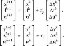
After determining the primal-dual direction $\mathrm{\Delta }{\mathit{{\rm X}}}_{\text{pd}}$ from (20), we compute primal and dual step lengths as follows:

$$\begin{array}{cc}& {\tau }_p^{\text{pd}}=0.9995\hspace{0.17em}\underset{i}{\min }\left\{{1,\frac{-l_i}{\mathrm{\Delta }{l}_{\text{pd}·i}}|}_{\mathrm{\Delta }{l}_{\text{pd}·i}<0},{\frac{-u_i}{\mathrm{\Delta }{u}_{\text{pd}·i}}|}_{\mathrm{\Delta }{u}_{\text{pd}·i}<0}\right\},\\ {\tau }_d^{\text{pd}}=0.9995\hspace{0.17em}\underset{i}{\min }\left\{{1,\frac{-z_i}{\mathrm{\Delta }{z}_{\text{pd}·i}}|}_{\mathrm{\Delta }{z}_{\text{pd}·i}<0},{\frac{-w_i}{\mathrm{\Delta }{w_{\text{pd}·}}_i}|}_{\mathrm{\Delta }{w}_{\text{pd}·i}>0}\right\}.\end{array}$$

(21)

After enlarging step lengths ${\tau }_p^{\text{pd}}$ and ${\tau }_d^{\text{pd}}$ to be ${\tilde{\tau }}_p$ and ${\tilde{\tau }}_d$ , respectively, we have

$$\begin{array}{cc}& \left[\begin{array}{c}\tilde{\mathit{l}}\\ \tilde{\mathit{u}}\end{array}\right]=\left[\begin{array}{c}\mathit{l}\\ \mathit{u}\end{array}\right]+{\tilde{\tau }}_p\left[\begin{array}{c}\mathrm{\Delta }{\mathit{l}}_{\text{pd}}\\ \mathrm{\Delta }{\mathit{u}}_{\text{pd}}\end{array}\right],\\ \left[\begin{array}{c}\tilde{\mathit{z}}\\ \tilde{\mathit{w}}\end{array}\right]=\left[\begin{array}{c}\mathit{z}\\ \mathit{w}\end{array}\right]+{\tilde{\tau }}_d\left[\begin{array}{c}\mathrm{\Delta }{\mathit{z}}_{\text{pd}}\\ \mathrm{\Delta }{\mathit{w}}_{\text{pd}}\end{array}\right].\end{array}$$

(22)

Let $\tilde{\mathit{v}}=\tilde{\mathit{L}}\tilde{\mathit{z}}$ , $H=[\sigma \tilde{g}\theta ,\sigma \tilde{g}/\theta ]$ , $\theta \in (\mathrm{0,1})$ , and

$$\begin{array}{l}\mathit{v}=\pi \left(\tilde{\mathit{v}}\mid H\right),\\ \text{where}\hspace{1em}{v}_i=\{\begin{array}{ll}{\tilde{v}}_i\hfill & {\tilde{v}}_i\in H\hfill \\ \sigma \tilde{g}\theta \hfill & {\tilde{v}}_i<\sigma \tilde{g}\theta \hfill \\ \frac{\sigma \tilde{g}}{\theta }\hfill & {\tilde{v}}_i>\frac{\sigma \tilde{g}}{\theta },\hfill \end{array}\\ \tilde{\mathit{\upsilon }}=\tilde{\mathit{U}}\tilde{\mathit{w}},\hspace{1em}\hspace{1em}\mathit{\upsilon }=-\pi \left(-\tilde{\mathit{\upsilon }}\mid H\right).\end{array}$$

(23)

Let ${\mathit{K}}_{\text{mcc}}=[0;0;0;0;\mathit{v}-\tilde{\mathit{v}};\mathit{\upsilon }-\tilde{\mathit{\upsilon }}]$ ; the centrality correction direction $\mathrm{\Delta }{\mathit{{\rm X}}}_{\text{mcc}}$ can be obtained by solving the following equation system:

$$\begin{array}{cc}& \mathit{M}\left(·\right)\mathrm{\Delta }{\mathit{{\rm X}}}_{\text{mcc}}={\mathit{K}}_{\text{mcc}}.\end{array}$$

(24)

Then the primal-dual and centrality correction directions are combined to be the total direction

$$\begin{array}{cc}& \mathrm{\Delta }\mathit{{\rm X}}=\mathrm{\Delta }{\mathit{{\rm X}}}_{\text{pd}}+\mathrm{\Delta }{\mathit{{\rm X}}}_{\text{mcc}}.\end{array}$$

(25)

If we consider the total direction $\mathrm{\Delta }\mathit{{\rm X}}$ as the new primal-dual direction $\mathrm{\Delta }{\mathit{{\rm X}}}_{\text{pd}}$ , a new centrality corrections step can be implemented again.

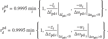
After computing primal and dual step lengths ${\tau }_p$ and ${\tau }_d$ for $\mathrm{\Delta }\mathit{{\rm X}}$ according to (21), the iterating points can be updated as follows:

$$\begin{array}{cc}& \left[\begin{array}{c}{\mathit{x}}^{k+\mathrm{1}}\\ {\mathit{l}}^{k+\mathrm{1}}\\ {\mathit{u}}^{k+\mathrm{1}}\end{array}\right]=\left[\begin{array}{c}{\mathit{x}}^k\\ {\mathit{l}}^k\\ {\mathit{u}}^k\end{array}\right]+{\tau }_p\left[\begin{array}{c}\mathrm{\Delta }{\mathit{x}}^k\\ \mathrm{\Delta }{\mathit{l}}^k\\ \mathrm{\Delta }{\mathit{u}}^k\end{array}\right],\\ \left[\begin{array}{c}{\mathit{y}}^{k+\mathrm{1}}\\ {\mathit{z}}^{k+\mathrm{1}}\\ {\mathit{w}}^{k+\mathrm{1}}\end{array}\right]=\left[\begin{array}{c}{\mathit{y}}^k\\ {\mathit{z}}^k\\ {\mathit{w}}^k\end{array}\right]+{\tau }_d\left[\begin{array}{c}\mathrm{\Delta }{\mathit{y}}^k\\ \mathrm{\Delta }{\mathit{z}}^k\\ \mathrm{\Delta }{\mathit{w}}^k\end{array}\right].\end{array}$$

(26)

The centering parameter σ is very important for IPM [4]. If $\sigma =1$ , the equation system (20) defines a centering direction, a Newton step toward the point at which all the pairwise products are identical to $\tilde{g}$ . At the other extreme, the value $\sigma =0$ gives the standard Newton step toward the point at which $g=0$ . There are several strategies to set σ. The first one is fixed strategy, which is a method setting $\sigma \in [\mathrm{0,1})$ and keeping σ unchanged during the iterations of IPM [4]. The other one is Mehrotra's predictor-corrector (MPC) method which determines the value of σ by using a preliminary step computation [5]. Now we give the details of MPC method. First, let ${\mathit{K}}_{\text{af}}=\mathit{K}(\mathit{X},\sigma \tilde{g})|{}_{\sigma =0}$ , and we have $\mathrm{\Delta }{\mathit{{\rm X}}}_{\text{af}}$ after solving $\mathit{M}(·)\mathrm{\Delta }{\mathit{{\rm X}}}_{\text{af}}=-{\mathit{K}}_{\text{af}}$ . We then compute affine step lengths ${\tau }_p^{\text{af}}$ and ${\tau }_d^{\text{af}}$ for $\mathrm{\Delta }{\mathit{{\rm X}}}_{\text{af}}$ according to (21). Next, we compute $g_{\text{af}}=(\mathit{l}+{\tau }_p^{\text{af}}\mathrm{\Delta }{\mathit{l}}_{\text{af}}{)}^T(\mathit{z}+{\tau }_d^{\text{af}}\mathrm{\Delta }{\mathit{z}}_{\text{af}})-(\mathit{u}+{\tau }_p^{\text{af}}\mathrm{\Delta }{\mathit{u}}_{\text{af}}{)}^T(\mathit{w}+{\tau }_d^{\text{af}}\mathrm{\Delta }{\mathit{w}}_{\text{af}})$ ; then $\sigma =(g_{\text{af}}/g{)}^3$ . The third strategy setting σ is LOQO method [24]. It defines σ as $\sigma =\mathrm{0.1}\times \min {(\rho (1-\xi )/\xi ,\stackrel{-}{\rho })}^{\mathrm{3}}$ , where $\xi ={\min }_i\{l_i{z}_i,-u_i{w}_i\}/\tilde{g}$ , $\rho =\mathrm{0.05}$ , and $\stackrel{-}{\rho }=\mathrm{2}$ .

5.2. Optimal Centering Parameter

The aforementioned methods of defining centering parameter are effective for solving linear programming, but all these methods are based on experience or experiment. In this subsection, we present a novel optimization model for σ, and the optimal σ can be obtained through minimizing the equilibrium distance-quality function (ED-QF) for the predicted iterating points.

Definition 2.

ED-QF for strict interior point X can be denoted as $d_{\text{exact}}^{\eta }(\mathit{X})={\parallel \mathit{K}(\mathit{X},\eta \tilde{g})\parallel }^2$ , where $\eta \in (\mathrm{0,1})$ .

The following points are obvious.

• (a)

$d_{\text{exact}}^{\eta }(\mathit{X})\to {\parallel \mathit{K}(\mathit{X},\tilde{g})\parallel }^2$ for $\eta \to \mathrm{1}$ , and ED-QF represents the distance between X and ${\mathit{X}}_{\tilde{g}}$ . ${\mathit{X}}_{\tilde{g}}$  satisfies $\mathit{K}({\mathit{X}}_{\tilde{g}},\tilde{g})=0$ .

(b)

$d_{\text{exact}}^{\eta }(\mathit{X})\to {\parallel \mathit{K}(\mathit{X},0)\parallel }^2$ for $\eta \to 0$ , and ED-QF represents the distance between X and the KKT point ${\mathit{X}}_{*}$ . ${\mathit{X}}_{*}$ satisfies $\mathit{K}({\mathit{X}}_{*},0)=0$ . It is important to note that, for $\eta =\mathrm{0},d_{\text{exact}}^{\eta }(\mathbf{X})$ is the equivalent of quality function in [26].

So ED-QF contains the centricity and optimization of X synchronously.

We are now in a position to give the model defining optimal σ. For iteration point X, the optimal σ is the one which minimizes the ED-QF of next iteration point $\widehat{\mathbf{X}}(\sigma )$ :

$$\begin{array}{cc}& \sigma =\underset{\sigma }{\text{argmin}}\left\{d_{\text{exact}}^{\eta }\left(\widehat{\mathit{X}}\left(\sigma \right)\right)\right\},\end{array}$$

(27)

where $d_{\text{exact}}^{\eta }(\widehat{\mathit{X}}(\sigma ))={\parallel L_{\mathit{x}}(\widehat{\mathit{X}}(\sigma ))\parallel }^2$ + ${\parallel L_{\mathit{y}}(\widehat{\mathit{X}}(\sigma ))\parallel }^2$ + ${\parallel L_{\mathit{z}}(\widehat{\mathit{X}}(\sigma ))\parallel }^2$ + ${\parallel L_{\mathit{w}}(\widehat{\mathit{X}}(\sigma ))\parallel }^2$ + ${\parallel L_{\mathit{l}}(\widehat{\mathit{X}}(\sigma ),\eta \tilde{g}(\sigma ))\parallel }^2$ + ${\parallel L_{\mathit{u}}(\widehat{\mathit{X}}(\sigma ),\eta \tilde{g}(\sigma ))\parallel }^2$ ,   $\widehat{\mathit{X}}(\sigma )=[\widehat{\mathit{x}}(\sigma );\widehat{\mathit{y}}(\sigma );\widehat{\mathit{z}}(\sigma );\widehat{\mathit{w}}(\sigma );\widehat{\mathit{l}}(\sigma );\widehat{\mathit{u}}(\sigma )]$ , $\widehat{\mathit{x}}(\sigma )=\mathit{x}+{\widehat{\tau }}_p(\sigma )\mathrm{\Delta }\widehat{\mathit{x}}(\sigma )$ , $\widehat{\mathit{y}}(\sigma )=\mathit{y}+{\widehat{\tau }}_d(\sigma )\mathrm{\Delta }\widehat{\mathit{y}}(\sigma )$ , $\widehat{\mathit{l}}(\sigma )=\mathit{l}+{\widehat{\tau }}_p(\sigma )\mathrm{\Delta }\widehat{\mathit{l}}(\sigma )$ , $\widehat{\mathit{z}}(\sigma )=\mathit{z}+{\widehat{\tau }}_d(\sigma )\mathrm{\Delta }\widehat{\mathit{z}}(\sigma )$ , $\widehat{\mathit{u}}(\sigma )=\mathit{u}+{\widehat{\tau }}_p(\sigma )\mathrm{\Delta }\widehat{\mathit{u}}(\sigma )$ , $\widehat{\mathit{w}}(\sigma )=\mathit{w}+{\widehat{\tau }}_d(\sigma )\mathrm{\Delta }\widehat{\mathit{w}}(\sigma )$ , $\mathrm{\Delta }\widehat{\mathit{{\rm X}}}(\sigma )=\mathrm{\Delta }{\mathit{{\rm X}}}_{\text{pd}}$ , ${\widehat{\tau }}_p(\sigma )$ , and ${\widehat{\tau }}_d(\sigma )$ are the step lengths for $\mathrm{\Delta }\widehat{\mathit{{\rm X}}}(\sigma )$ .

The evaluation of $d_{\text{exact}}^{\eta }(\widehat{\mathbf{X}}(\sigma ))$ is, however, expensive since it requires the evaluation of the problem functions and derivatives for every value of σ. We can avoid this expense by using a linear technique. Because $f(·)$ , $\mathit{h}(·)$ , and $\mathit{g}(·)$ are continuous and differentiable for our SLDPCL model, we have

$$\begin{array}{l}\hspace{0.17em}f\left(\widehat{\mathit{x}}\left(\sigma \right)\right)\approx f\left(\mathit{x}\right)+\nabla f{\left(\mathit{x}\right)}^T\left(\widehat{\mathit{x}}\left(\sigma \right)-\mathit{x}\right)\\ =f\left(\mathit{x}\right)+\nabla f{\left(\mathit{x}\right)}^T{\widehat{\tau }}_p\left(\sigma \right)\mathrm{\Delta }\widehat{\mathit{x}}\left(\sigma \right),\\ \mathit{h}\left(\widehat{\mathit{x}}\left(\sigma \right)\right)\approx \mathit{h}\left(\mathit{x}\right)+\nabla \mathit{h}{\left(\mathit{x}\right)}^T\left(\widehat{\mathit{x}}\left(\sigma \right)-\mathit{x}\right)\\ =\mathit{h}\left(\mathit{x}\right)+\nabla \mathit{h}{\left(\mathit{x}\right)}^T{\widehat{\tau }}_p\left(\sigma \right)\mathrm{\Delta }\widehat{\mathit{x}}\left(\sigma \right),\\ \hspace{0.17em}\mathit{g}\left(\widehat{\mathit{x}}\left(\sigma \right)\right)\approx \mathit{g}\left(\mathit{x}\right)+\nabla \mathit{g}{\left(\mathit{x}\right)}^T{\widehat{\tau }}_p\left(\sigma \right)\mathrm{\Delta }\widehat{\mathit{x}}\left(\sigma \right),\\ \hspace{0.17em}\nabla f\left(\widehat{\mathit{x}}\left(\sigma \right)\right)\approx \nabla f\left(\mathit{x}\right),\\ \hspace{0.17em}\nabla \mathit{h}\left(\widehat{\mathit{x}}\left(\sigma \right)\right)\approx \nabla \mathit{h}\left(\mathit{x}\right),\\ \hspace{0.17em}\nabla \mathit{g}\left(\widehat{\mathit{x}}\left(\sigma \right)\right)\approx \nabla \mathit{g}\left(\mathit{x}\right),\\ \hspace{0.17em}\mathit{H}\left(\widehat{\mathit{X}}\left(\sigma \right)\right)\approx 0.\end{array}$$

(28)

According to (16)–(19) and (28), we have

$$\begin{array}{l}{\parallel L_{\mathit{x}}\left(\widehat{\mathit{X}}\left(\sigma \right)\right)\parallel }^{\mathrm{2}}\\ \hspace{1em}=\parallel -\nabla f\left(\widehat{\mathit{x}}\left(\sigma \right)\right)+\nabla \mathit{h}\left(\widehat{\mathit{x}}\left(\sigma \right)\right)\widehat{\mathit{y}}\left(\sigma \right)\\ {\hspace{1em}\hspace{1em}\hspace{1em}+\nabla \mathit{g}\left(\widehat{\mathit{x}}\left(\sigma \right)\right)\left(\widehat{\mathit{z}}\left(\sigma \right)+\widehat{\mathit{w}}\left(\sigma \right)\right)\parallel }^2\\ \hspace{1em}\approx \parallel -\nabla f\left(\mathit{x}\right)+\nabla \mathit{h}\left(\mathit{x}\right)\left(\mathit{y}+{\widehat{\tau }}_d\left(\sigma \right)\mathrm{\Delta }\widehat{\mathit{y}}\left(\sigma \right)\right)\\ {\hspace{1em}\hspace{1em}\hspace{0.5em}+\nabla \mathit{g}\left(\mathit{x}\right)\left(\mathit{z}+{\widehat{\tau }}_d\left(\sigma \right)\mathrm{\Delta }\widehat{\mathit{z}}\left(\sigma \right)+\mathit{w}+{\widehat{\tau }}_d\left(\sigma \right)\mathrm{\Delta }\widehat{\mathit{w}}\left(\sigma \right)\right)\parallel }^2\\ \hspace{1em}=\parallel -\nabla f\left(\mathit{x}\right)+\nabla \mathit{h}\left(\mathit{x}\right)\mathit{y}+\nabla \mathit{g}\left(\mathit{x}\right)\left(\mathit{z}+\mathit{w}\right)\\ \hspace{1em}\hspace{1em}\hspace{0.5em}+{\widehat{\tau }}_d\left(\sigma \right)(\nabla \mathit{h}\left(\mathit{x}\right)\mathrm{\Delta }\widehat{\mathit{y}}\left(\sigma \right)\\ {\hspace{1em}\hspace{1em}\hspace{0.5em}+\nabla \mathit{g}\left(\mathit{x}\right)\left(\mathrm{\Delta }\widehat{\mathit{z}}\left(\sigma \right)+\mathrm{\Delta }\widehat{\mathit{w}}\left(\sigma \right)\right))\parallel }^2\\ \hspace{1em}=\left(\mathrm{1}-{\widehat{\tau }}_d\left(\sigma \right)\right){\parallel L_{\mathit{x}}\left(\mathit{X}\right)\parallel }^{\mathrm{2}},\\ {\parallel L_{\mathit{y}}\left(\widehat{\mathit{X}}\left(\sigma \right)\right)\parallel }^2={\parallel \mathit{h}\left(\widehat{\mathit{x}}\left(\sigma \right)\right)\parallel }^2\\ \approx {\parallel \mathit{h}\left(\mathit{x}\right)+{\widehat{\tau }}_p\left(\sigma \right)\nabla \mathit{h}{\left(\mathit{x}\right)}^T\mathrm{\Delta }\widehat{\mathit{x}}\left(\sigma \right)\parallel }^2\\ =\left(1-{\widehat{\tau }}_p\left(\sigma \right)\right){\parallel L_{\mathit{y}}\left(\mathit{X}\right)\parallel }^2,\\ {\parallel L_{\mathit{z}}\left(\widehat{\mathit{X}}\left(\sigma \right)\right)\parallel }^2\\ \hspace{1em}={\parallel \mathit{g}\left(\widehat{\mathit{x}}\left(\sigma \right)\right)-\widehat{\mathit{l}}\left(\sigma \right)-\underset{\_}{\mathit{g}}\parallel }^2\\ \hspace{1em}\approx {\parallel \mathit{g}\left(\mathit{x}\right)-\mathit{l}-\underset{\_}{\mathit{g}}+{\widehat{\tau }}_p\left(\sigma \right)\left(\nabla \mathit{g}{\left(x\right)}^T\mathrm{\Delta }\widehat{\mathit{x}}\left(\sigma \right)-\mathrm{\Delta }\widehat{\mathit{l}}\left(\sigma \right)\right)\parallel }^2\\ \hspace{1em}=\left(1-{\widehat{\tau }}_p\left(\sigma \right)\right){\parallel L_{\mathit{z}}\left(\mathit{X}\right)\parallel }^2,\\ \hspace{0.17em}{\parallel L_{\mathit{w}}\left(\widehat{\mathit{X}}\right(\sigma \left)\right)\parallel }^2\approx \left(1-{\widehat{\tau }}_p\left(\sigma \right)\right){\parallel L_{\mathit{w}}\left(\mathit{X}\right)\parallel }^2.\end{array}$$

(29)

According to (29) and $\tilde{g}(\sigma )\approx \sigma \tilde{g}$ , ED-QF for $\widehat{\mathit{X}}(\sigma )$ can be approximated as

$$\begin{array}{l}d\text{approx}.\eta \left(\widehat{\mathit{X}}\left(\sigma \right)\right)=\left(1-{\widehat{\tau }}_d\left(\sigma \right)\right){\parallel L_{\mathit{x}}\left(\mathit{X}\right)\parallel }^2+\left(1-{\widehat{\tau }}_p\left(\sigma \right)\right)\\ \times \left({\parallel L_{\mathit{y}}\left(\mathit{X}\right)\parallel }^2+{\parallel L_{\mathit{z}}\left(\mathit{X}\right)\parallel }^2+{\parallel L_{\mathit{w}}\left(\mathit{X}\right)\parallel }^2\right)\\ +{\parallel \mathit{L}\left(\sigma \right)\mathit{Z}\left(\sigma \right)\mathit{e}-\eta \sigma \tilde{g}\parallel }^2\\ +{\parallel \mathit{U}\left(\sigma \right)\mathit{W}\left(\sigma \right)\mathit{e}+\eta \sigma \tilde{g}\parallel }^2\approx d_{\text{exact}}^{\eta }\left(\widehat{\mathit{X}}\left(\sigma \right)\right).\end{array}$$

(30)

Note that $\mathrm{\Delta }\widehat{\mathit{{\rm X}}}(\sigma )=\mathrm{\Delta }\widehat{\mathit{{\rm X}}}(0)+\sigma (\mathrm{\Delta }\widehat{\mathit{{\rm X}}}(1)-\mathrm{\Delta }\widehat{\mathit{{\rm X}}}(0))$ . Therefore, after solving linear system (20) twice to obtain $\mathrm{\Delta }\widehat{\mathit{{\rm X}}}(0)$ and $\mathrm{\Delta }\widehat{\mathit{{\rm X}}}(1)$ , we can get $\mathrm{\Delta }\widehat{\mathit{{\rm X}}}(\sigma )$ easily for any value of σ. Then, the dominant computational overhead in the evaluation of $d_{\text{approx}.}^{\eta }(\widehat{\mathit{X}}(\sigma ))$ lies in the computation of the maximal step lengths for $\mathrm{\Delta }\widehat{\mathit{{\rm X}}}(\sigma )$ and the last two terms in (30), which require a few simple vector operations. We implement a one-dimensional search scheme, based on a golden trisection procedure, for $\sigma \in [{\sigma }_{\min },{\sigma }_{\max }]$ , to obtain an approximate minimizer of $d_{\text{approx}.}^{\eta }(\widehat{\mathit{X}}(\sigma ))$ .

Algorithm OCP.

Initialization. ${\sigma }_{\min }=\mathrm{0},\mathrm{\hspace{0.17em}\hspace{0.17em}}{\sigma }_{\max }=\mathrm{100}$ , $k_{\sigma }=\mathrm{1}$ , $\widehat{r}=\mathrm{0.618}$ , $\widehat{l}=\mathrm{0.382}$ , $k_{\sigma }^{\max }=\mathrm{10}$ , $\varpi =\mathrm{0.1}$ .

Step 1.

Compute $\mathrm{\Delta }\widehat{\mathit{{\rm X}}}(0)$ and $\mathrm{\Delta }\widehat{\mathit{{\rm X}}}(1)$ .

Step 2.

If $d_{\text{approx}.}^{\eta }(\widehat{\mathit{X}}(0.99))<d_{\text{approx}.}^{\eta }(\widehat{\mathit{X}}(1))$ , then ${\sigma }_{\max }=1$ ; otherwise ${\sigma }_{\min }=1$ .

Step 3.

${\sigma }_r={\sigma }_{\min }+\widehat{r}({\sigma }_{\max }-{\sigma }_{\min })$ , $f_{lr}=\widehat{r}$ .

Step 4.

If $f_{lr}=\widehat{r}$ , then ${\sigma }_l={\sigma }_{\min }+\widehat{l}({\sigma }_{\max }-{\sigma }_{\min })$ ; if $f_{lr}=\widehat{l}$ , then ${\sigma }_r={\sigma }_{\min }+\widehat{r}({\sigma }_{\max }-{\sigma }_{\min })$ .

Step 5.

If $d_{\text{approx}.}^{\eta }(\widehat{\mathit{X}}({\sigma }_l))<d_{\text{approx}.}^{\eta }(\widehat{\mathit{X}}({\sigma }_r))$ , then ${\sigma }_{\max }={\sigma }_r$ , ${\sigma }_r={\sigma }_l$ , $f_{lr}=\widehat{r}$ ; otherwise ${\sigma }_{\min }={\sigma }_l$ , ${\sigma }_l={\sigma }_r$ , $f_{lr}=\widehat{l}$ .

Step 6.

If $k_{\sigma }<k_{\sigma }^{\max }$ and ${\sigma }_{\max }-{\sigma }_{\min }>\varpi {\sigma }_{\max }$ , then $k_{\sigma }=k_{\sigma }+1$ , goto Step 4; otherwise $\sigma =({\sigma }_{\min }+{\sigma }_{\max })/\mathrm{2}$ is the optimal centering parameter, stop.

5.3. Improved IPM

Algorithm Improved IPM (I-IPM)

Initialization. $k=0$ , $\epsilon =10^{-5}$ ; η, δ, γ, $\theta \in (\mathrm{0,1})$ , and in this paper $\eta =0.05$ , $\delta =0.2$ , $\gamma =0.05$ , $\theta =0.2$ ;  and ${\mathit{X}}^0$ .

Step 1.

If ${\parallel \mathit{K}({\mathit{X}}^k,0)\parallel }^2\le \epsilon$ , where $\mathit{K}({\mathit{X}}^k,0)$ is defined according to (15), ${\mathit{X}}^k$ is optimal and stop.

Step 2.

Compute σ by using Algorithm OCP and let $\mathrm{\Delta }{\mathit{{\rm X}}}_{\text{pd}}=\mathrm{\Delta }\widehat{\mathit{{\rm X}}}(0)+\sigma (\mathrm{\Delta }\widehat{\mathit{{\rm X}}}(1)-\mathrm{\Delta }\widehat{\mathit{{\rm X}}}(0))$ .

Step 3.

Compute the step lengths ${\tau }_p^{\text{pd}}$ and ${\tau }_d^{\text{pd}}$ for $\mathrm{\Delta }{\mathit{{\rm X}}}_{\text{pd}}$ according to (21).

Step 4.

MCC procedure.

Step  4.1. Set $k_{\text{mcc}}^{\max }=\mathrm{5}$ .

Step  4.2. ${\tilde{\tau }}_p=\min ((\mathrm{1}+\delta ){\tau }_p^{\text{pd}},\mathrm{1}),{\tilde{\tau }}_d=\min ((\mathrm{1}+\delta ){\tau }_d^{\text{pd}},\mathrm{1})$ .

Step  4.3. Compute $\mathrm{\Delta }{\mathit{{\rm X}}}_{\text{mcc}}$ according to (24), compute $\mathrm{\Delta }\mathit{{\rm X}}$ according to (25) and compute step lengths ${\tau }_p$ and ${\tau }_d$ for $\mathrm{\Delta }\mathit{{\rm X}}$ according to (21).

Step  4.4. If the number of corrections less than $k_{\text{mcc}}^{\max }$ and ${\tau }_p\ge (\mathrm{1}+\gamma \delta ){\tau }_p^{\text{pd}}$ or ${\tau }_d\ge (\mathrm{1}+\gamma \delta ){\tau }_d^{\text{pd}}$ , then $\mathrm{\Delta }{\mathit{{\rm X}}}_{\text{pd}}=\mathrm{\Delta }\mathit{{\rm X}}$ , ${\tau }_p^{\text{pd}}={\tau }_p$ , and ${\tau }_d^{\text{pd}}={\tau }_d$ , goto Step 4.2.

Step 5.

According to (26), update the iteration point by using $\mathrm{\Delta }\mathit{{\rm X}}$ , ${\tau }_p$ and ${\tau }_d$ , $k=k+1$ , goto Step 1.

6. Computational Results and Complexity

6.1. Computational Results and Analysis

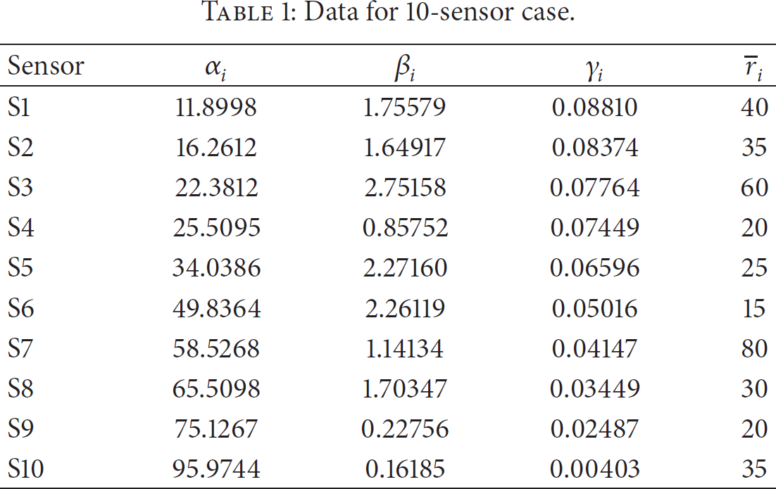
In this subsection we present some numerical results to test the impact of the separable formulation for the SLDPCL and the effectiveness of the proposed approaches. The machine on which we perform all of our computations is a Pentium (R) Dual Core 2.7 GHz Lenovo-PC computer with 2GB RAM, running MS-Windows 7, and Matlab 2010b. In the implementation of our algorithm, OAM described in Section 3, MILP master problem has been solved by calling MOSEK 6, while NLP problems have been solved by using Algorithm I-IPM. Test cases with sensors ranging from 10 to 20000 are used for simulation. Data of 10-sensor case are all listed in Table 1 and $x_{\text{all}}=150$ . The data of the other cases are created by duplicating the ten-sensor base data, whereas the length of line to cover is adjusted in proportion to the case size. Set $\epsilon ={10}^{-2}$ for OAM and set accuracy of the MILP solver MOSEK allowed to stop to be 0.1%.

Table 1

Data for 10-sensor case.

Sensor	${\alpha }_i$	${\beta }_i$	${\gamma }_i$	${\stackrel{-}{r}}_i$
S1	11.8998	1.75579	0.08810	40
S2	16.2612	1.64917	0.08374	35
S3	22.3812	2.75158	0.07764	60
S4	25.5095	0.85752	0.07449	20
S5	34.0386	2.27160	0.06596	25
S6	49.8364	2.26119	0.05016	15
S7	58.5268	1.14134	0.04147	80
S8	65.5098	1.70347	0.03449	30
S9	75.1267	0.22756	0.02487	20
S10	95.9744	0.16185	0.00403	35

The Algorithm OAM is carried out for two different models (7) (nonseparated) and (10) (separated), which are denoted as OAM (primal OAM) and S-OAM (separated OAM), respectively. We first compare the tightness of the outer approximation master problems (8) and (11). The results are displayed in Table 2, which presents the lower bound at the first iteration for each strategy. The column “q” reports the total number of sensors, while columns “Va-(8)” and “Va-(11)” report the optimal values of the outer approximation master problems (8) and (11) at the first iteration, respectively. The results show that, as expected, the outer approximation of a separated equivalent is tighter than the direct outer approximation of the original multivariate problem.

Table 2

Comparison of 2 models in tightness.

q	Va-(8)	Va-(11)
10	490.3616	498.5428
20	992.1475	1003.2713
30	1488.2213	1431.4722
40	1985.7825	2018.3667
50	2481.8563	2522.4782
60	2976.4431	3029.1279
70	3472.5163	3529.9108
80	3968.5901	4036.1891
90	4464.6638	4539.6210
100	4911.0632	4996.1190

The results of 10-sensor case are listed in Table 3. Note that once $x_i$ is given for all $i\in Q$ (we will have $x_i=0$ for those sensors that are not selected), it is trivial to find the set of optimal locations: just align the discs so that they do not intersect and they cover the entire line. For this purpose we choose the diameters in such a way that their sum is equal to the length of the line, which in our case is equal to $x_{\text{all}}=\mathrm{150}$ . An illustration of a feasible solution to 10-sensor case is given in Figure 1.

Table 3

Results of 10-sensor case.

Sensor	S1	S2	S3	S4	S5	S6	S7	S8	S9	S10
$r_i$	13.16	13.95	0	20.00	0	0	47.88	0	20.00	35.00

Figure 1

Illustration of 10-sensor case.

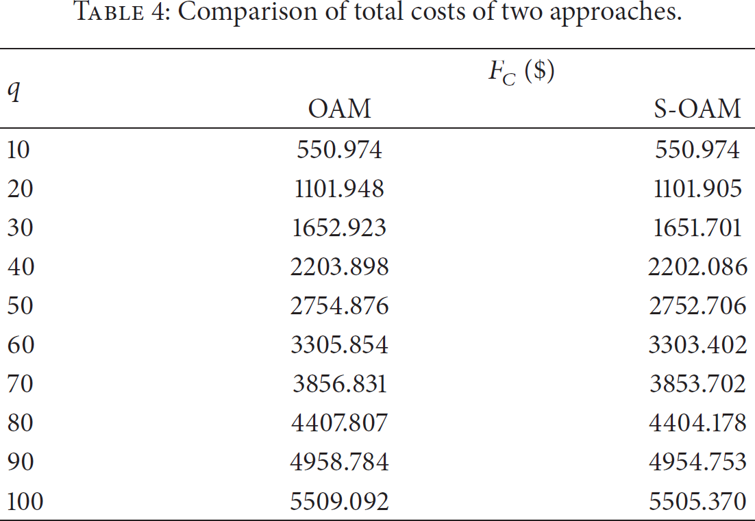
In addition, for the purpose of comparison, we implement OAM, S-OAM two different strategies on the test cases with sensors ranging from 10 to 100. The comparison of the total costs of the two approaches is presented in Table 4. “ $F_C$ ” denotes the total cost. As it can be seen, the S-OAM can find higher-quality solutions in comparison with OAM.

Table 4

Comparison of total costs of two approaches.

q	$F_C$ ($)
	OAM	S-OAM
10	550.974	550.974
20	1101.948	1101.905
30	1652.923	1651.701
40	2203.898	2202.086
50	2754.876	2752.706
60	3305.854	3303.402
70	3856.831	3853.702
80	4407.807	4404.178
90	4958.784	4954.753
100	5509.092	5505.370

We note that (6) is a mixed integer quadratic programming (MIQP), which can be solved by many efficient general-purpose mixed integer programming solvers such as MOSEK, CPLEX, and GUROBI. We solve (6) with MOSEK directly by setting the accuracy to 0.1 and 0.05, which are the relative optimality tolerances employed by the solver. The comparison of the results between MOSEK and our approach is presented in Table 5, where columns “ $C_{\text{time}}$ ” and “ $N_{\text{it}}$ ” denote the execution time and number of iterations, respectively. As it can be observed, S-OAM can find better solutions within similar order of time as MOSEK, during which no more than five iterations have been executed, while the accuracy in MOSEK is 0.1. When accuracy of MOSEK is set to 0.05, S-OAM gets the same high-quality solutions as MOSEK for all cases but with less execution time. To sum up, S-OAM is better than MOSEK in both accuracy cases.

Table 5

Comparison of S-OAM and MOSEK.

	Solving (6) with MOSEK				S-OAM
q	Accuracy 0.1		Accuracy 0.05
	$F_C$ ($)	$C_{\text{time}}$ (s)	$F_C$ ($)	$C_{\text{time}}$ (s)	$F_C$ ($)	$C_{\text{time}}$ (s)	$N_{\text{it}}$
10	564.800	6.4	550.974	11.3	550.974	7.3	3
50	2789.234	12.9	2754.876	30.7	2752.706	10.2	3
100	5557.353	21.3	5510.091	59.2	5505.370	19.7	4
200	11090.62	24.7	11019.97	89.1	11010.43	22.6	5
500	28076.57	31.5	27529.88	202.7	27526.08	20.0	3
1000	55523.13	40.8	55069.23	290.6	55052.14	34.1	4
5000	280352.2	631.9	275261.38	2031.9	273061.2	279.0	5
10000	557846.9	2177.8	—	—	550521.9	627.6	3
20000	—	—	—	—	1100965.9	1124.8	5

“—” denotes that MOSEK cannot reach the preset accuracy for this instance within preset 3600 seconds.

Perspective function is a well-known tool in convex analysis. By using this tool, Frangioni reformulate SLDPCL as an MISOCP [3]. And it can be solved by using MOSEK too. To test the efficiency of the proposed method, we further compare it with MISOCP method [3]. We set the termination tolerance to 0.05 for MOSEK. The comparison of the results between MISOCP and our approach is presented in Table 6. And Table 6 shows that solving MISOCP with MOSEK for SLDPCL takes 2-3 times longer running time or even more than our method when the quality of the solutions is of the same level.

Table 6

Comparison of S-OAM and MISOCP.

q	MISOCP [3]		S-OAM
	$F_C$ ($)	$C_{\text{time}}$ (s)	$F_C$ ($)	$C_{\text{time}}$ (s)
10	550.974	5.2	550.974	7.3
50	2752.706	14.6	2752.706	10.2
100	5513.722	31.1	5505.370	19.7
200	11016.25	47.6	11010.43	22.6
500	27547.62	114.9	27526.08	20.0
1000	55052.17	151.7	55052.14	34.1
5000	275505.30	713.2	273061.2	279.0
10000	550587.91	1821.0	550521.9	627.6
20000	—	—	1100965.9	1124.8

“—” denotes that MOSEK cannot reach the preset accuracy for this instance within preset 3600 seconds.

The average operation cost for one sensor (shown in Figure 2) is an important factor to validate the proposed method. In Figure 2, lines “MOSEK-0.1” and “MOSEK-0.05” report the results of solving (6) with MOSEK directly by setting the accuracy to 0.1 and 0.05, respectively; line “MISOCP” reports the results of solving MISOCP model of SLDPCL, while line “S-OAM” reports the results of proposed method. As can be seen in Figure 2, the average operation costs provided by proposed method are lower than the ones provided by other methods for all cases.

Figure 2

Comparison of cost per sensor with the number of sensors.

Figure 3 depicts the relationship between the CPU time and the number of sensors for three methods. The execution times used by proposed method increase nearly linearly as the number of sensors increases (Figure 3), while the other three lines sharply go up as the number of sensors increases. Figure 3 shows that the proposed method suits large-scaled SLDPCL problems.

Figure 3

CPU time with the number of sensors.

There are two NLPs in Steps 1 and 3 of Algorithm OAM, which are solved with the Algorithm I-IPM presented in Section 4. We will show the efficiency of the proposed novel I-IPM in the following paragraphs.

After deleting Step 4 from Algorithm I-IPM, set $\sigma =0.1$ , set σ according to LOQO method, set σ according to MPC method, or set σ to be optimal centering parameter; we obtain 4 different IPMs, denoted as PDIPM [4], LOQO [24], MPC [5], and ED-QF, respectively. When $q=100$ , it is shown in Figure 4 that all the average step lengths (average of the primal and dual step lengths) are taken in every iteration by different IPMs for solving the relaxation of (7). It can be seen in Figure 4 that ED-QF generally takes a larger step length than the other IPMs, which leads to better convergence.

Figure 4

Comparison of 4 algorithms in the average step length.

When different IPM was used to solve the relaxation of (7) for our proposed S-OAM algorithm, Table 7 gives the number of iterations to convergence and CPU times for the PDIPM [4], PCIPM [5], and I-IPM algorithms. It is obvious that I-IPM dominates the other IPMs both in number of iterations and CPU times.

Table 7

Comparison of 3 IPMs in results.

q	$N_{\text{it}}$ / $C_{\text{time}}$ (s)
	PDIPM [4]	PCIPM [5]	I-IPM
100	23/0.13	18/0.13	12/0.12
200	25/0.24	22/0.28	14/0.23
500	23/0.61	20/0.62	13/0.51
1000	28/1.90	23/1.64	14/1.20
5000	33/12.77	24/9.81	14/6.63
10000	36/27.12	22/18.04	15/13.84
20000	35/51.04	22/39.67	13/26.19
Sum	203/93.81	151/70.19	95/48.72

6.2. Complexity Estimate

In full generality, SLDPCL is a challenging optimization problem, as SLDPC combines the difficulty of optimizing over integer variables with the handling of nonlinear functions. As pointed in [14], it is NP-hard problem. In our method, we reduce this NP-hard problem to MILP and convex NLP. The convex NLP can be solved efficiently by using proposed I-IPM in polynomial times. MILP can be solved by using the off-the-shelf MILP solvers effectively, although it is an NP-hard problem as well. Then, the complexity of proposed method depends on three aspects. The first one is complexity of I-IPM. Let $ϵ\in (\mathrm{0,1})$ be given. Suppose that I-IPM for solving NLP generates a sequence of iterates that satisfies ${\mu }_{k+1}\le (1-\varrho /n^{\omega }){\mu }_k$ , $k=\mathrm{0,1},2,\dots$ , for some positive constants ϱ and ω. Suppose that the starting point satisfies ${\mu }_0\le 1/{ϵ}^{\kappa }$ for some positive constant κ. Then the I-IPM can obtain a solution satisfying ${\mu }_k\le ϵ$ with no more than $O(n^{\omega }\left|\log ϵ\right|)$ iterations. The similar proof can be found in [27]. The second aspect of complexity of S-OAM is the complexity of solving MILP, which is an NP-hard problem. The last one is the iterations number of S-OAM, which is a hard open problem for MINLP. So, it is very hard to estimate accurately the complexity of the proposed method.

7. Conclusions

SLDPCL problems come from many application problems in common with tremendous number of variables and constraints. In this paper, we combine OAM and IPM and give a novel S-OAM for SLDPCL. Our algorithm can get good CPU time and high-quality solutions. Furthermore, our S-OAM approach could be improved in at least two ways: (a) by using the preprocessing procedure in order to fix on some binary variables before the calling of our algorithm; (b) by embedding I-IPM in a branch-and-cut approach, like that of MOSEK, in order to improve the efficiency of solving sub-problems.