Modeling the Performance of Faulty Linear Wireless Sensor Networks

Abstract

Wireless sensor networks (WSNs) are used to monitor long linear structures such as pipelines, rivers, railroads, international borders, and high power transmission cables. In this case, a special type of WSN called linear wireless sensor network (LSN) is used. One of the main challenges of using LSNs is the reliability of the connections across the nodes. Faults in a few contiguous nodes may cause the creation of holes (segments where nodes on either end of them cannot reach each other) which will result in dividing the network into multiple disconnected segments. As a result, sensor nodes that are located between holes may not be able to deliver their sensed information which negatively affects the network's sensing coverage. In this paper, we provide an analysis of the different types of node faults in uniformly deployed LSNs and study their negative impact on the sensing coverage. We develop an analytical model to estimate the sensing coverage in uniformly deployed sensors LSNs in the presence of node faults. We verify the correctness of the developed model by conducting a number of simulation experiments to compare both calculated and simulated results under different network configurations and fault scenarios. In addition, we use this model to demonstrate three design applications that meet with specific performance requirements.

1. Introduction

The advent of communication and computer technologies has resulted in many innovations such as the development of low cost, low power, easily deployable, and self-organized wireless sensors. This technology opens great opportunities for a wide array of monitoring applications such as environmental, industrial, and security applications. Some of the applications involve monitoring linear structures that could extend for hundreds of kilometers in harsh or uninhabited environments. The WSNs used for monitoring this type of infrastructures are called linear wireless sensor networks (LSNs). A LSN differs from a WSN in various aspects. For example, WSN routing is usually complex and several approaches such as shortest multipath methods [1] may be used, while, in LSNs, the structure dictates exactly two possible routing paths (to the left or right of a node). However, WSNs can handle failures and loads in a relatively better way given the different options for route selection and maintenance as the example model demonstrates in [2]. Yet, in LSNs, failures may cause more severe problems, and drastic solutions need to be considered to discover and recover from faults since there are no possible path alternatives. Typical applications of LSNs include monitoring water, oil, and gas pipelines; rivers; railways; international borders; and high power transmission cables [3]. Each sensor node is equipped with the necessary sensing elements, a battery, a wireless transceiver, a low-capability processor, a small memory, and a small storage unit. The sensors are lined through the structure to provide three main functions: sensing, information relay, and information filtering. The sensing function is to observe any interesting changes in or around the monitored structure. The information relay helps forward the observed data to the main station using multihop communication. The filtering function filters out unwanted data and aggregates multiple pieces of sensed data into smaller messages. This optimizes communication, processing, and routing as well as the power needs, thus extending the life of the LSN.

WSNs are generally designed to have good coverage [4–6]. However, the special way LSNs are designed results in a major challenge of losing connectivity in the network in the presence of multiple node faults [7]. This is due to faults in neighboring and consecutive nodes. Nodes can fail due to battery exhaustion, hardware failures, and natural or intentional damage. These consecutive faulty nodes form holes which may cause the LSN to be divided into multiple disconnected segments. Some of these segments will become isolated; thus, they cannot transfer their sensed data to the main station. As a result, the isolated segments will not provide any sensing coverage.

In this paper, we study the types of faults in uniformly deployed LSNs, where nodes are distributed at uniform distances, and the impact of these faults on the sensing coverage. We develop an analytical model to estimate coverage in LSNs in the presence of node faults. We verify the correctness of the developed model by conducting a number of simulation experiments to compare both calculated and simulated results under different network configurations and fault scenarios. This analytical model can be used to analyze LSN designs and to help plan maintenance schedules for a LSN. One example of this LSN is the one used for monitoring underwater pipelines [8]. Underwater pipelines extend for hundreds of kilometers at depths reaching hundreds of meters and are subjected to high pressure [9]. At such depths, it is really difficult to perform maintenance activities for the LSN. Periodic maintenance is needed to recover from accidental LSN faults to maintain good sensing coverage. In addition, the developed model can be used to evaluate new LSN designs or to compare different possible designs that can be developed for monitoring linear structures.

The rest of the paper is organized as follows. Section 2 discusses the related work. Section 3 provides some background information about LSN. Section 4 discusses the different types of faults in LSN and the impact of these faults on the sensing coverage. Section 5 develops an analytical model to estimate the coverage in the presence of node faults. Section 6 provides experimental validations of the model, while Section 7 discusses some potential applications for the developed model. Section 8 concludes the paper with remarks about the main contributions and planned future work.

2. Related Work

Different aspects of LSN have been investigated recently by researchers. The applications, issues, and classifications of LSN were surveyed in [3, 7]. In addition, a number of efficient routing protocols [10] and a distributed topology discovery algorithm [11] for LSN were developed. Zimmerling et al. studied energy-efficient and localized power-aware routing in LSN [12, 13]. Noori and Ardakani proposed an analysis to characterize the traffic load distribution over a randomly deployed LSN [14]. Liu et al. provided an algorithm for an energy-balanced data gathering for LSN [15]. Li and Shunjie provided energy-efficient node replacement schemes in LSN to balance network load and extend network lifetime [16]. Finally, Martin and Paterson developed a lightweight key redistribution mechanism for LSN [17].

The coverage problem was one of the important issues of WSN that recently got high attention [4–6]. Some of the research was dedicated for developing approaches that can achieve high coverage [18–22], while other work was dedicated for developing analytical models and optimization techniques for high WSN coverage [23–27]. However, all of these efforts covered randomly deployed two- and three-dimensional WSN. LSNs represent a special case of WSN that has its own unique characteristics and coverage problems. None of the mentioned works studied the coverage problem in LSN which is important for some critical infrastructure applications such as pipeline, long power line, river, and highway monitoring.

3. Background

Wireless sensor networks offer coverage for geometrical areas in various shapes and sizes and as nodes are distributed over the area, multipath routing and other coverage models can be used to offer the best possible coverage in the presence of failures or security threats. For example, the authors in [28] tackle the issue of topology control to minimize the node set needed to monitor a specific area. Further, [29] aims to achieve the same goal by relying on the ability to change the sensing radius of the nodes. The use of sensing node in this manner covers a large range of application domains. However, in some cases, the areas to be monitored can be of a specific shape or size such that a special type of WSNs may be used. One of the most common special structures is the linear structure. In this case, sensing nodes are placed in a linear fashion along the structure. This type of WSN is usually called the linear WSN (LSN) and it is the focus of our work in this paper.

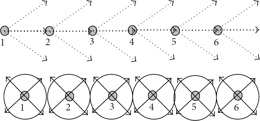
In a LSN, like in WSN in general, sensing nodes usually have limited transmission compatibilities where each node can communicate with only a few neighboring nodes. Nodes collaborate among themselves in both sensing and communication functions. Multihop communication is used to transfer the sensed and control data across the linear structure and to/from the main control station and other control points that may be distributed over the structure. Wireless networks can solve some of the reliability problems of current wired networks technologies that are used to monitor linear structures [30]. For example, WSNs can still function even when some nodes are disabled. Faults in sensor nodes can be easily tolerated using other available nodes to cover the faulty ones. Using dense WSNs with a high number of nodes and/or using wide wireless transmission ranges, the network can maintain connectivity and the sensed and control data can be transmitted through the network to their destination even with the existence of some node faults. For example, each node in Figure 1 can communicate with two nodes to the left and two nodes to the right. If, for example, nodes 3 and 5 are damaged, node 4 can still send its sensed data through node 2 or 6. The maximum number of neighboring nodes that each node can communicate with each side can be defined as a maximum jump factor (MJF). For example, MJF in Figure 1 is 2; thus node 4 can communicate with a maximum of two nodes on each side.

Figure 1

Reliability in a dense LSN.

Each sensor node is usually equipped with a transceiver, a processor, a battery, memory, and small storage in addition to one or more sensing elements. Power consumption is critical to the life span of LSNs. Linear structures need to be monitored throughout their life span which could extend to tens of years. Therefore, the associated LSNs should also be long lived. Unlike wired networks where the power is not at all a constraint as the wires deliver power to the different sensor nodes, LSN designers have to consider power as one of the main constraints in the wireless system. Power in a sensing node is consumed by every element on it. A transceiver consumes power waiting for a signal and when transmitting or receiving data. Sensing elements also consume power and the processor as well. Careful scheduling of these resources is needed to optimize power consumption. Although increasing the transmission range can provide better communication reliability, more energy will be consumed by the nodes. A dynamic configuration for the wireless transmission range can provide better power management. An example of this configuration is in Figure 2. In this network, nodes 3 and 5 have failed. Therefore, the wireless range for node 4 is increased to reach nodes 2 and 6, while other nodes use a smaller transmission range to reduce the power consumption.

Figure 2

Automatic wireless range configuration.

The sensed data is transferred through the line to the main station in either direction or both if both directions are connected to the main station. Connecting both directions to the main station will double the communication reliability [9, 31]. In LSNs, a node can be considered a faulty node even if it functions but cannot communicate with any nodes from both directions due to insufficient energy. In this case, the node can sense but cannot communicate or forward any sensed data and can be considered as a faulty node.

4. Sensing Coverage in LSN

Sensor nodes are usually initially distributed to cover the whole linear structure in terms of both sensing and communication coverage. A node senses interesting events and this observation is reported to the main station using multihop communication. Sensors in LSN nodes can have different sensing range capabilities. In a uniform LSN where nodes are distributed at uniform distances, let us define the distance between two neighboring nodes i and $i+1$ as one distance unit. Then, a LSN with healthy nodes can provide 100% sensing coverage for the monitored linear structures if the node sensing range (NSR) is one distance unit. Figure 3 shows examples of two LSNs with NSR equal to one distance unit. The difference between the two LSNs is that the nodes in the top LSN sense in one direction (like a stationary camera) while the nodes of the LSN in the bottom sense in all directions (such as sound capturing).

Figure 3

Two LSNs with $\text{NSR}=1$ . Top LSN: each node senses in one direction. Bottom LSN: each node senses in all directions.

This coverage is reduced if there are some faulty nodes. However, if NSR is larger than d (one distance unit), then some node faults can be easily tolerated without reducing the percentage of the sensing coverage. For example, if NSR is 2 distance units, this means that the area between two neighboring nodes i and $i+1$ is monitored twice by both nodes. In this case, this area will be still under monitoring even if node i or node $i+1$ is faulty.

LSN is usually designed to provide a full sensing coverage. However, after some time, there will be some faults among the nodes. Let us consider that we have a one-segment network with homogeneous nodes. Let us also assume that there is a uniform distance between each two nodes. In addition, nodes have a specific MJF. Let us define a term hole $(H)$ as the number of contiguous faulty nodes in the LSN. Each hole can be of size one or more nodes. For example, in Figure 4, we have two holes: $H_1$ and $H_2$ . The first one is with size 1 where only node 2 is faulty, while the second hole, $H_2$ , is of size 3 where nodes 5, 6, and 7 are faulty. We use $Z(H_1)=1$ and $Z(H_2)=3$ , where Z is the size function of a hole. In addition, we can use $(H_i)=[F_i:L_i]$ to specify the ID of first faulty node, $F_i$ , and the ID of last faulty node, $L_i$ , in $H_i$ . Thus, we have $Z(H_i)=L_i-F_i+1$ .

Figure 4

Two holes in the LSN.

A special type of hole is a disconnecting hole $(\text{DH})$ , which disconnects the network into two segments that can not directly communicate with each other using an extended wireless range. In other words, the size of a $\text{DH}$ is larger than or equal to the MJF used for the nodes in the LSN, $Z(\text{DH})\ge \text{MJF}$ . For example, if the MJF of the LSN in Figure 4 is 2, then $H_2$ is $\text{DH}$ while $H_1$ is not. This is because $Z(H_2)=3$ which is larger than the MJF, while $Z(H_1)=1$ which is less than the MJF.

There are different types of faults in a one-segment LSN with homogenous nodes distributed uniformly over the linear structure. Assuming that both ends of the LSN are connected to the main station, the faults have different impacts on the communication and sensing coverage.

Fault Type 1—There Are Multiple Holes, Where All Are Not Disconnecting Holes. In this case, the LSN will function normally. Although there will be some holes with sizes smaller than MJF, any sensed information can be transferred to the main station through the left or right side of the network. Any hole can be jumped over by extending the wireless range of the node that forwards the sensed data to the MJF to reach the next functioning node. The sensing coverage in each hole may or may not be affected. This depends on the size of the hole and $\text{NSR}$ . Let $U(H_i)$ be the size of the uncovered sensing area in $H_i$ . Consider

$$\begin{array}{cc}& U\left(H_i\right)=\{\begin{array}{cc}\mathrm{0}\hfill & Z\left(H_i\right)<\text{NSR}\hfill \\ Z\left(H_i\right)-\left(\text{NSR}-\mathrm{1}\right)\hfill & \text{Otherwise}.\hfill \end{array}\end{array}$$

(1)

For example, if $Z(H_i)$ is 3 and NSR is 4, then $U(H_i)$ is 0. In another, if $Z(H_i)$ is 6 and NSR is 3, then $U(H_i)$ is 4. If there are n nodes and k holes in a LSN, then the sensing coverage percentage, C, is

$$\begin{array}{cc}& C=\frac{n-{\sum }_{i=\mathrm{1}}^{k}U\left(H_i\right)}{n}.\end{array}$$

(2)

Fault Type 2—There Are Multiple Holes, Where Only One of Them Is a Disconnecting Hole. In this case, the LSN will continue to function. This one $\text{DH}$ will divide the LSN into two segments: one on the left side of the $\text{DH}$ and the other is on the right side. As the size of the $\text{DH}$ is larger than or equal to MJF, then this $\text{DH}$ will disable information exchange between both segments as shown in Figure 5. In this case, all healthy nodes on the left side of the $\text{DH}$ will use a right-to-left forwarding direction, while all healthy nodes on the right side will use a left-to-right forwarding direction to communicate with the main station. As in fault type 1, any small hole can be jumped over by extending the wireless range of the node that forwards the information.

Figure 5

LSN with $\text{MJF}=2$ . LSN is divided into two segments by a DH. Each one will communicate in a different direction.

The sensing coverage of LSN can be calculated using (1) and (2) as in fault type 1. In the example shown in Figure 6, the size of $\text{DH}$ is 3 while $\text{NSR}$ is 4; then the whole area of $\text{DH}$ is covered by healthy nodes 6 and 10. In another example (see Figure 7), the size of $\text{DH}$ is 5 while $\text{NSR}$ is 4. In this case, there are 2 distance units that are not covered by both healthy nodes 6 and 12.

Figure 6

LSN with $\text{MJF}=2$ . $Z(\text{DH})=3$ and $\text{NSR}=4$ . The whole $\text{DH}$ is covered.

Figure 7

LSN with $\text{MJF}=2$ . $Z(\text{DH})=5$ and $\text{NSR}=4$ . The whole $\text{DH}$ is not covered.

Fault Type 3—There Are Multiple Holes, Where Only Two of Them Are Disconnecting Holes. In this case, the LSN will be divided into three segments. Let the $\text{DH}$ s be DH₁ and DH₂. The first segment is before DH₁, the second segment is between DH₁ and DH₂, and the third segment is after DH₂ as shown in Figure 8. In this figure, DH₁ is from node 5 to node 6, while DH₂ is from node 11 to node 13. The first segment covers nodes 1 through 4, the second covers nodes 7 through 10, and the third covers nodes 14 through 17. All nodes in the first segment can communicate with the main station in the right-to-left direction, while all nodes in the third segment can communicate with the main station in the left-to-right direction. However, healthy nodes in the second segment cannot communicate with the main station at all.

Figure 8

LSN with $\text{MJF}=2$ . There are two DHs: DH₁ and DH₂. The segment between DH₁ and DH₂ is not connected.

The effect of this type of fault is similar to having a large $\text{DH}$ , DH_1,2, that extends from node 5 to node 13. Let $({\text{DH}}_1)=[F_1:L_1]$ and let $R({\text{DH}}_2)=[F_2:L_2]$ ; then, $R({\text{DH}}_{\mathrm{1,2}})=[F_1:L_2]$ and $Z({\text{DH}}_{\mathrm{1,2}})=L_2-F_1+1$ . The parameters of the new composite $\text{DH}$ , DH_1,2, can be used to find uncovered areas and the coverage percentage defined in (1) and (2). In the example in Figure 8, we have $({\text{DH}}_{\mathrm{1,2}})=[F_1:L_2]=[5:13]$ and $Z({\text{DH}}_{\mathrm{1,2}})=L_2-F_1+1=13-5+1=9$ .

Fault Type 4—There Are Multiple Holes with More Than Two Disconnecting Holes. Let us assume that there are k DHs: DH₁ through ${\text{DH}}_k$ . This means that the LSN will be divided into $k+1$ segments. With the existence of k DHs, all nodes starting from the first node in DH₁ to the last in ${\text{DH}}_k$ will not be able to communicate with the main station. As a result, the areas from DH₁ to ${\text{DH}}_k$ will be uncovered. An example is shown in Figure 9. In this example, the LSN consists of 17 nodes. There are three $\text{DH}$ s and four segments. The first segment includes nodes 1 and 2, the second includes nodes 5 and 6, the third includes nodes 9 through 11, and the fourth includes nodes 15 through 17. All nodes in the first segment can communicate with the main station on their left and all nodes in the fourth segment can communicate with the main station on their right. All nodes in the middle segments cannot communicate with the main station. In reality, the whole area from the first node in DH₁ to the last node in DH₃ will not be covered.

Figure 9

LSN with $\text{MJF}=2$ and with three DHs. The area from the first to the third will not be covered.

The effect of this type of fault is similar to having a large $\text{DH}$ , ${\text{DH}}_{1,k}$ , that expands from the first node in DH₁ to the last node in ${\text{DH}}_k$ . Let $({\text{DH}}_1)=[F_1:L_1]$ and let $R({\text{DH}}_k)=[F_j:L_k]$ ; then, $R({\text{DH}}_{1,k})=[F_1:L_k]$ and $Z({\text{DH}}_{1,k})=L_k-F_1+1$ . The parameters of the new composite $\text{DH}$ , ${\text{DH}}_{1,k}$ , can be used to find uncovered areas as well as the coverage percentage as defined in (1) and (2).

5. Coverage Modeling

In this section, a sensing coverage analytical model is developed for linear wireless sensor networks with the presence of node faults. Table 1 defines some parameters that are used in the modeling. To understand the impact of faults on the LSN, we will start with simple faults of two disconnecting holes; then, we will cover the general case with multiple disconnecting holes.

Table 1

Defined modeling parameters.

Parameter	Description
n	Network size (number of nodes)
MJF	Maximum jump factor
NSR	Node sensing range
f	Node fault probability
k	Number of disconnecting holes
C	Coverage percentage
$U_i$	The size of the uncovered sensing area in a hole with size i
${\text{CA}}_k$	Expected connected area
${\text{DA}}_k$	Expected disconnected area
EC	Expected coverage

Two disconnecting holes in a LSN can have different impact levels on the coverage. This depends on their locations in the LSN. The worst case is when both holes are located very far from each other at the opposite ends of the LSN. In this case, the whole network will be disconnected from the main station and all nodes in the network will not be able to send their sensed information. The best case is when both holes are located very close to each other at any location. In this case, only the area from the first hole to second hole will be uncovered, while all other parts will be connected to the main station. The average case which can be generally used for evaluation is shown in Figure 8. The result of this case is like dividing the LSN into three equal sized segments. The first hole is between the first and second segments, while the second hole is between the second and third segments. Both first and third segments will be connected to the main station and covered, while the second segment will not be connected and will be uncovered. For a network with two small disconnected holes, the coverage will be reduced to around two-thirds of the full coverage.

Similar to the two-hole case, the occurrence of multiple disconnecting holes in a LSN can have different impact levels on the coverage. This depends on their locations. The worst case is when two of the disconnecting holes are very far from each other at the opposite ends of the LSN. In this case, the whole network will be disconnected from the main station and all nodes in the network will not be able to send their sensed information. In contrast, the best case is when all holes are located very close to each other. In this case, only the area from the first disconnecting hole to the last disconnecting hole will be uncovered, while all other parts will be connected to the main station and covered. The average case is like dividing the network into $(k+1)$ equal sized segments where there are k disconnecting holes. Each disconnecting hole disconnects two neighboring segments. In this case, only the first and the last segments will be connected to the main station and their areas are covered, while all other segments are not connected and their areas are not covered. Thus, the coverage will be reduced to $2/(k+1)$ of the full coverage. Let the network size be n and let the expected coverage with zero holes, EC₀, be 100 percent; then, if there are k small disconnected holes, then the expected coverage ${\text{EC}}_k$ will be reduced to

$$\begin{array}{cc}& {\text{EC}}_K=\frac{\mathrm{2}}{k+\mathrm{1}}.\end{array}$$

(3)

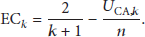
If there are k small disconnecting holes, the LSN will be divided into two kinds of expected percentages: expected connected area $({\text{CA}}_k)$ and expected disconnecting area $({\text{DA}}_k)$ . The connected area contains the connected parts on both ends of the LSN, while the disconnected area is the disconnecting part that contains all disconnecting holes and the segments of the network between those holes. We have

$$\begin{array}{cc}& {\text{CA}}_k+{\text{DA}}_k=\mathrm{1}.\end{array}$$

(4)

To find the values of ${\text{CA}}_k$ and ${\text{DA}}_k$ , we use (3) which provides expected coverage percentage and also represents the percentage of the expected connected area as follows:

$$\begin{array}{cc}& {\text{CA}}_k=\frac{\mathrm{2}}{k+\mathrm{1}},\end{array}$$

(5)

$$\begin{array}{cc}& {\text{DA}}_k=\mathrm{1}-\frac{\mathrm{2}}{k+\mathrm{1}}=\frac{k-\mathrm{1}}{k+\mathrm{1}}.\end{array}$$

(6)

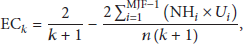
Now, (3) does not include uncovered subareas due to holes that are not disconnecting holes (holes) in the connected area. Although these will not have high impact on the coverage, we can include them for better estimation. All holes with sizes 1 to 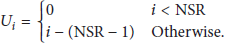$\text{MJF}-1$ are holes. Let ${\text{NH}}_i$ be the number of holes of size i in the whole LSN. Based on (5), if we have k disconnecting holes, the expected connected area percentage will be ${\text{CA}}_k$ . This means that the number of holes with sizes i in the connected area is ${\text{NH}}_i·{\text{CA}}_k$ . From (1), the uncovered area $U_i$ from a hole with size i is

$$\begin{array}{cc}& U_i=\{\begin{array}{cc}\mathrm{0}\hfill & i<\text{NSR}\hfill \\ i-\left(\text{NSR}-\mathrm{1}\right)\hfill & \text{Otherwise}.\hfill \end{array}\end{array}$$

(7)

Now, the expected total of uncovered area from all holes with sizes i that are located in the connected area is ${\text{NH}}_i·{\text{CA}}_k·U_i$ . From this equation, we can find the expected total of all holes located in the connected area, $U_{\text{CA},k}$ , as follows:

$$\begin{array}{cc}& U_{\text{CA},k}={\displaystyle \sum }_{i=\mathrm{1}}^{\text{MJF}-{\mathrm{1}}^{\prime }}\left({\text{NH}}_i\times {\text{CA}}_k\times U_i\right).\end{array}$$

(8)

We can use this equation to adjust (3) to include uncovered areas not only due to the disconnecting holes but also due to holes located in the connected area as follows:

$$\begin{array}{cc}& {\text{EC}}_k=\frac{\mathrm{2}}{k+\mathrm{1}}-\frac{U_{\text{CA},k}}{n}.\end{array}$$

(9)

We replace $U_{\text{CA},k}$ with (8); we get

$$\begin{array}{cc}& {\text{EC}}_k=\frac{\mathrm{2}}{k+\mathrm{1}}-\frac{{\sum }_{i=\mathrm{1}}^{\text{MJF}-\mathrm{1}}\left({\text{NH}}_i\times {\text{CA}}_k\times U_i\right)}{n}.\end{array}$$

(10)

We replace ${\text{CA}}_k$ with (5); we get

$$\begin{array}{cc}& {\text{EC}}_k=\frac{\mathrm{2}}{k+\mathrm{1}}-\frac{\mathrm{2}{\sum }_{i=\mathrm{1}}^{\text{MJF}-\mathrm{1}}\left({\text{NH}}_i\times U_i\right)}{n\left(k+\mathrm{1}\right)},\end{array}$$

(11)

$$\begin{array}{cc}& {\text{EC}}_k=\frac{\mathrm{2}}{k+\mathrm{1}}\left(\mathrm{1}-\frac{{\sum }_{i=\mathrm{1}}^{\text{MJF}-\mathrm{1}}\left({\text{NH}}_i\times U_i\right)}{n}\right).\end{array}$$

(12)

Equations (3) and (12) show direct links between the number of disconnecting holes and the expected coverage. In this section, we will also find the expected number of holes. Given a LSN with n uniformly distributed nodes and a specific MJF, each node has a chance to independently fail with probability f within a certain period T. T can be the time to a periodic full maintenance or the time that the LSN is needed to live. There is a need to find the expected number of holes that will occur and their sizes within the time T. Let us first find the probability equation when a healthy node in the LSN has a hole directly in front of it with exactly size i. We name this equation $W_{f,i}$ :

$$\begin{array}{cc}& W_{f,i}={\left(\mathrm{1}-f\right)}^2\times f^i.\end{array}$$

(13)

Here, as f increases, the chance to have a healthy node with a hole in front of it with size i also increases. As there are n nodes in the LSN and all nodes other than the last i node, which has no chance to have a hole in front of it, have the same chance to have a hole in front of them, then the number of holes in the LSN with size i is

$$\begin{array}{cc}& {\text{NH}}_i=W_{f,i}\times \left(n-i\right).\end{array}$$

(14)

We have

$$\begin{array}{cc}& {\text{NH}}_i={\left(\mathrm{1}-f\right)}^2\times f^i\times \left(n-i\right).\end{array}$$

(15)

Here, as the LSN size increases, the chance to have more holes in the LSN also increases.

A realistic value of f is generally very low as the probability to have holes with sizes larger than a certain number in a LSN is very small. For example, if there are 1000 nodes with 20% node fault probabilities, based on (15), the expected number of holes with size 11 is very small: 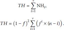$1.31\times {10}^{-5}$ . Therefore, we can consider that we have a variable v that represents the maximum size of possible holes. The total expected number of holes in the network is

$$\begin{array}{cc}& TH={{\displaystyle \sum }}_{i=\mathrm{1}}^v{\text{NH}}_i,\\ TH={\left(\mathrm{1}-f\right)}^{\mathrm{2}}{{\displaystyle \sum }}_{i=\mathrm{1}}^v\left(f^i\times \left(n-i\right)\right).\end{array}$$

(16)

The total expected number of disconnecting holes is

$$\begin{array}{cc}& k={{\displaystyle \sum }}_{i=\text{MJF}}^v{\text{NH}}_i,\end{array}$$

(17)

$$\begin{array}{cc}& k={\left(\mathrm{1}-f\right)}^{\mathrm{2}}{{\displaystyle \sum }}_{i=\text{MJF}}^v\left(f^i\times \left(n-i\right)\right).\end{array}$$

(18)

Generally, the value of variable v is enough to be 10 for most cases. However, this number can be increased for more accurate results. As the majority of holes will be small, we can use ${\text{NH}}_i$ from (15) and k from (18) in (12) to find the expected coverage percentage with the presence of faults as

$$\begin{array}{cc}& \text{EC}=\frac{\mathrm{2}}{k+\mathrm{1}}\left(\mathrm{1}-\frac{{\left(\mathrm{1}-f\right)}^{\mathrm{2}}{\sum }_{i=\mathrm{1}}^{\text{MJF}-\mathrm{1}}\left(f^i\times \left(n-i\right)\times U_i\right)}{n}\right),\end{array}$$

(19)

where we can get k from (18) and $U_i$ from (7). Equation (19) is valid if k is equal to or larger than 1. Otherwise, if k is less than 1, this means there is no hole and the coverage stays at high level.

6. Validations

A set of simulation experiments was conducted to validate the analytical model developed in the previous section. The experiments compare the calculated and simulated coverages of LSNs. Each LSN will be initially deployed to provide full coverage. However, after some time, some faults will occur in some nodes, thus reducing the coverage in the LSN. In this case, the LSN needs maintenance to regain full coverage again. The simulations were developed using Java, where experimental situations were created with 10,000 LSNs that were generated randomly to have different types of faults for each situation. The results are the averages measured from all these faulty LSNs.

The first experiment validates the expected coverage result of LSN with two disconnecting holes; a simulation experiment was conducted for different LSN sizes to allow us to compare the calculated and simulated results. The simulation was developed using 10,000 faulty LSNs, each with two disconnecting holes at randomly generated locations. The size of both disconnecting holes was 2, while MJF was also 2. The results were the averages measured from all these faulty LSNs. The results of both calculated and simulated coverages are shown in Figure 10. As we can see, the results are matched for all LSN sizes. This also shows that the expected coverage percentage is reduced to around 66.7% of the full coverage.

Figure 10

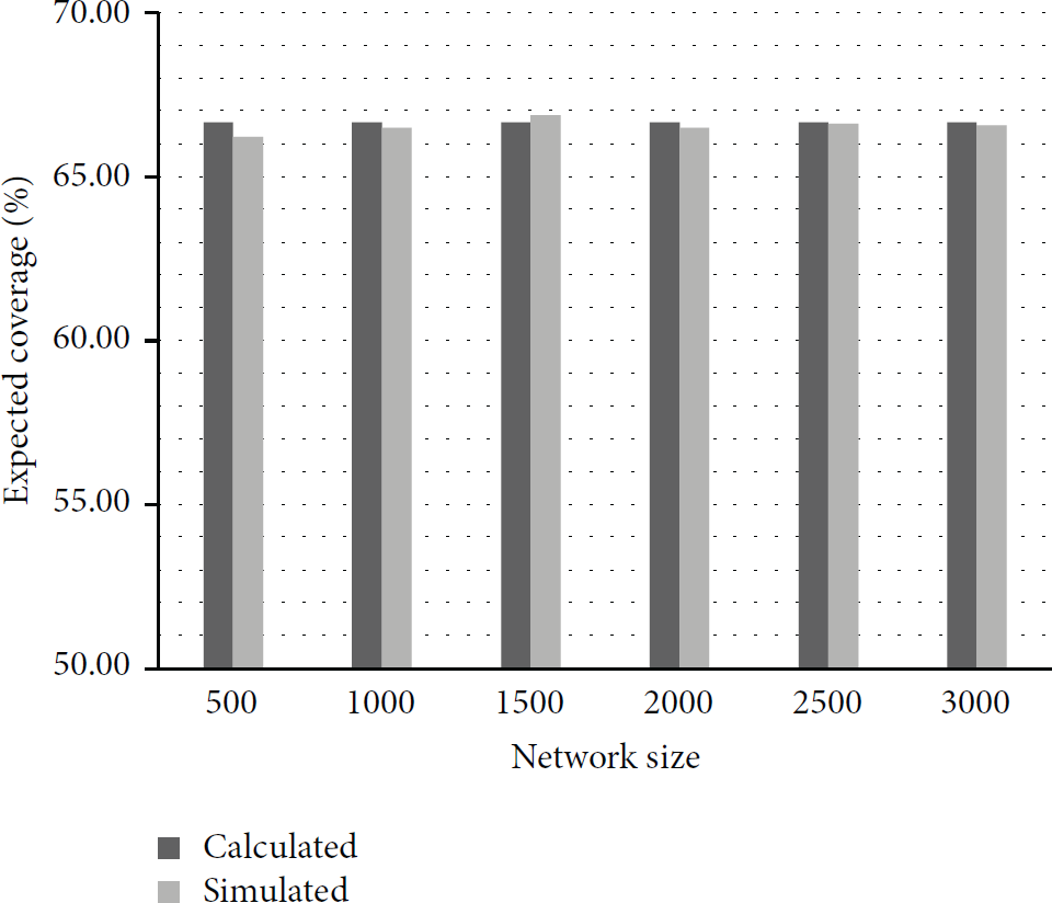
Expected coverage percentage for different sizes of LSNs with two disconnecting holes.

To validate (3) for the expected coverage with k disconnected holes, simulation experiments were conducted to compare the calculated and simulated results. The first experiment was conducted for different LSN sizes with 4 disconnecting holes. The experimental situations were created with 10,000 faulty LSNs, each with four disconnecting holes at randomly generated locations. The size of the disconnecting holes was 2, while MJF was also 2. The results were the averages measured from all these faulty LSNs. The results of both calculated and simulated coverages are shown in Figure 11. As we can see, the results are matched for all LSN sizes. This also shows that the expected coverage percentage is reduced to around 40% of the full coverage.

Figure 11

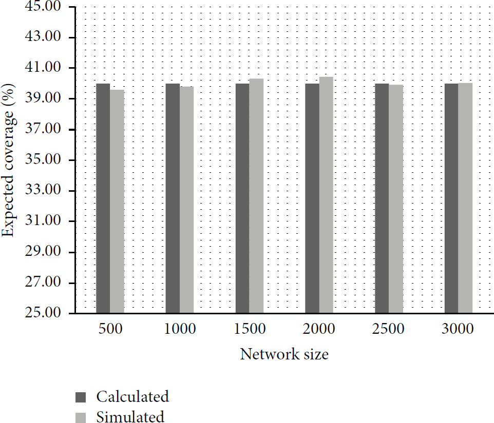
Expected coverage percentage for different sizes of LSNs with four disconnecting holes.

The second experiment was conducted to find the expected coverage percentage for a LSN with 1000 nodes under different numbers of disconnecting holes. The results are shown in Figure 12, where we have the simulated results and the calculated results calculated in (3). As we can see, both simulated and calculated results are very similar, which validates (3). The results also show that as the number of disconnecting holes increases the expected coverage of the LSN decreases.

Figure 12

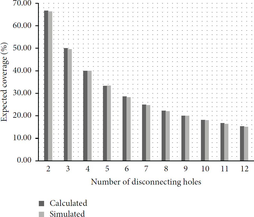
Expected coverage percentage for 1000-node LSN.

The third experiment was conducted to validate the number of holes (15). Here, as the LSN size increases, the chance to have more holes in the LSN also increases. Figure 13 shows the calculated and simulated numbers of holes in a 1000-node LSN with a node fault probability of 20%. As we can see, the holes sizes are small even with high node fault probabilities. In this example, all holes are mostly of sizes less than 5 nodes.

Figure 13

Number of calculated and simulated holes in 1000-node LSN with 20% node fault probability.

To verify the developed expected coverage (19), a set of four experiments was conducted. These experiments were developed to compare the results of the equation with the simulation results. The first experiment compares the coverage under different node fault probabilities. The network size used is 5000 nodes, MJF is 2, and NSR is 2. Both calculated and simulated cases were conducted for different node fault probabilities starting from 5% to 20%. This large range was selected to ensure some occurrence of disconnecting holes. The results are shown in Figure 14.

Figure 14

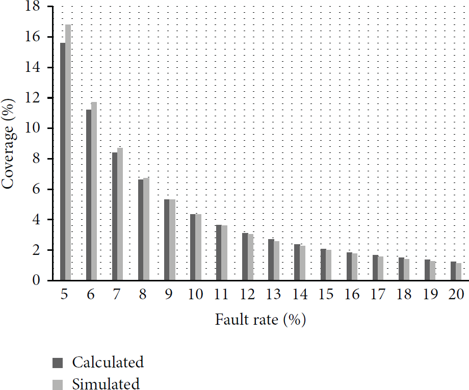
Coverage under different node fault probabilities. Number of nodes = 5000, $\text{MJF}=2$ , and $\text{NSR}=2$ .

The second experiment compares the coverage under different MJF values. Here, networks with sizes 5000 nodes were used with the node fault probabilities at 30%. These high fault probabilities were selected to make sure several disconnecting holes will occur. The experiment was conducted for MJF values from 2 to 5, while NSR was kept as 2. Both calculated and simulated results are very similar as shown in Figure 15. As we can notice, as MJF increases, the reliability and the coverage are significantly enhanced. The coverage is enhanced more than 3 times by increasing MJF from 4 to 5.

Figure 15

Coverage under different $\text{MJF}$ values. Nodes = 5000, $\text{NSR}=2$ , and fault probability = 30%.

The third experiment compares the coverage under different NSR values of 1 through 4. Here, networks of size 5000 were also used. The MJF was 4, while the node fault probability was 30%. Both calculated and simulated results are very similar and are shown in Figure 16. It is noticeable that the coverage increases with the increase of NSR. However, there is no significant increase when we have NSR greater than or equal to MJF. The main reason of this is that, as we have NSR greater than or equal to MJF, there will be more areas that are covered by multiple sensors and as a result the total coverage will not be enhanced.

Figure 16

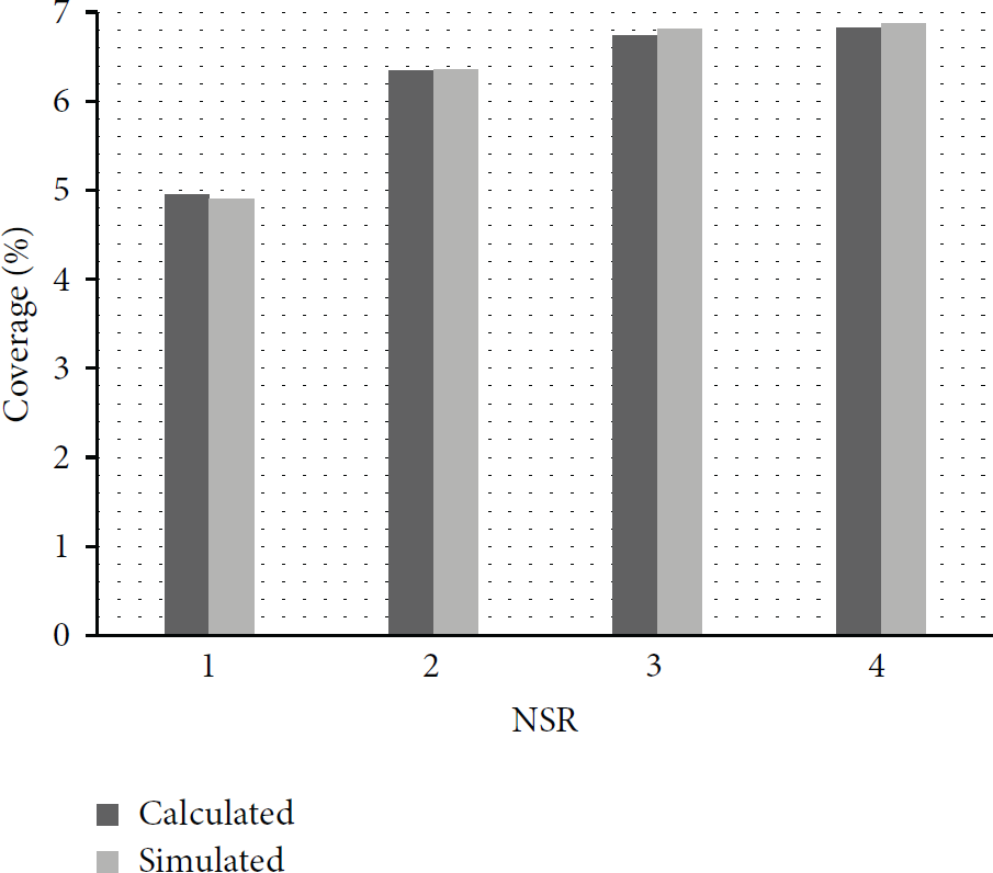
Coverage under different $\text{NSR}$ values. Nodes = 5000, $\text{MJF}=4$ , and fault probability = 30%.

The fourth experiment compares the coverage under different network sizes, from 500 nodes to 5000 nodes. For all these sizes, MJF was 2, NSR was 2, and node fault probability was 15%. Both calculated and simulated results are very similar as shown in Figure 17. The results show that, as we increase the network size, the coverage will be reduced since the overall failure possibility across all nodes becomes higher.

Figure 17

Coverage under different network sizes. $\text{MJF}=2$ , $\text{NSR}=2$ , and node fault probability = 15%.

7. Applications

The developed analytical model can be used in a number of applications. In this section, we will discuss three possible applications. The first is to estimate a periodic maintenance schedule for existing LSNs. The second is to use the model to create new reliable LSN designs. The third is to use the model to design a reliable LSN with multiple sinks.

7.1. Periodic Maintenance Schedule

Each LSN has specific parameters such as the number of nodes, MJF, and NSR. In addition, the percentage of monthly fault probabilities for the nodes is also known. Accordingly, we could estimate the best intervals for the periodic maintenance for the LSN such that it will always provide a high percentage of coverage. Let us assume that, during the periodic maintenance, all faulty nodes will be replaced with new nodes. This type of schedule is very important for critical applications such as long underwater pipelines where a periodic maintenance is required to ensure the safety of the pipeline [8, 9]. At the same time, it is really very difficult and costly to do instant maintenance for any incident after its occurrence.

Let us consider two LSNs: Network₁ and Network₂, generated from (19). Network₁ has 1000 nodes, MJF of 1, NSR of 2, and monthly fault probability of 1%. Network₂ has 2000 nodes, MJF of 3, NSR of 2, and monthly fault probability of 2%. Here, we assume that the fault probability will increase linearly with each passing month without maintenance. We use this particular fault model to demonstrate the problem; however, other realistic fault models can be used. As shown in Figure 18, the coverage of Network₁ starts declining after three months. Thus, it is good to schedule the regular periodic maintenance to replace faulty nodes every three months. On the other hand, the coverage of Network₂ starts declining after four months. As a result, it is good to schedule the periodic maintenance every four months.

Figure 18

Two LSN coverages without any maintenance.

7.2. LSN Design

Another application for the developed analytical model is LSN design. Assume that a linear structure of 25,000 meters long requires monitoring with a LSN for a period of four years. There are two types of sensor nodes available for this kind of monitoring. Both nodes use solar-energy to provide self-power for their operations. Both nodes were designed to have a maximum wireless range (MWR) of 200 meters and a maximum sensing coverage (MSC) of 100 meters. The first node type is a high quality model with fault probability of 5% during four years of operations, while the second type is of a lower quality with a high fault probability of 19% during four years. The price of first type is double the price of the second type. Which of the node types should be selected for the LSN that should provide more than 97% coverage during the four-year period? How many nodes should be used to meet the 97% coverage?

To select the best sensor node type and the number of nodes needed, we need to compare the different designs. Before we start, let us derive the formulas for NSR and MJF. We have here

$$\begin{array}{cc}& \text{MJF}=\frac{\text{MWR}}{\mathrm{2}\times \text{Total}\mathrm{\hspace{0.17em}\hspace{0.17em}}\text{Distance}/n},\\ \text{NSR}=\frac{\text{MSC}}{\text{Total}\mathrm{\hspace{0.17em}\hspace{0.17em}}\text{Distance}/n}.\end{array}$$

(20)

We need NSR to be at least equal to 1 for full coverage; thus, we need to use at least 250 nodes. If we use 250 nodes of the first type, then we have to use double this number of the second type (500 nodes) resulting in equal costs. Here, we will have MJF of 1 with first type and MJF of 2 with the second type as we doubled the number of nodes. An alternative design is to use 500 nodes of the first type to get NSR of 2 and MJF of 2. The total price of this design is similar to using 1000 nodes of the second type. In this case, we will have NSR of 4 and MJF of 4. Table 2 provides coverage results of different designs generated from (19). In each row, we have two equal-cost designs, one for the first node type and another for the second type. As we can see, the best suitable design is to use 1000 nodes of the second type. In this case, we will have an expected coverage of 97.5% during the specified period. This meets the LSN requirement specification. Although we can further increase the number of nodes to provide better coverage, this will increase the total cost, while there is no need to have such high coverage requirement.

Table 2

Different possible designs.

Number	Sensor node type 1				Sensor node type 2
	n	MJF	NSR	EC	n	MJF	NSR	EC
1	250	1	1	15.6%	500	2	2	12.9%
2	500	2	2	91.6%	1000	4	4	97.5%
3	750	3	3	100%	1500	6	6	100%

7.3. Reliable Design with Multiple Sinks

Multiple sinks can be used within a LSN to enhance the connectivity reliability of long LSNs. The sinks can be distributed at different distances among a long LSN to collect information from the close sensor nodes as shown in Figure 19. In this type of LSN, the network is divided into multiple small segments and, at the ends of each segment, there are two sinks to collect the sensed information from the sensor nodes. The main advantage of this network is that the sensed information does not need to pass through a long path to reach the main station. In addition, the overall reliability of the network can be enhanced as the reliability of a small LSN is better than a large LSN as shown in Section 6. A LSN with n nodes can be divided into h small segments. In this case, there are g nodes in each segment and $(h+1)$ sinks. We have g is equal to $n/h$ .

Figure 19

LSN with multiple sinks.

Given a specific LSN and specific sensor node characteristics, it is important to know how many sinks are needed to maintain high connectivity reliability and sensing coverage. Let us assume that we have a LSN with n nodes and each node has a specific MJF, NSR, and fault probability $(f)$ within a specific period T. The question here is how many sinks need to be embedded in the LSN to maintain high coverage within the period T. To solve this design question, we need to uniformly distribute the sinks such that there is a low probability of forming disconnecting holes between any two consecutive sinks within the period T. We can consider (18) but we replace n with g as each segment will have g nodes:

$$\begin{array}{cc}& k={\left(\mathrm{1}-f\right)}^{\mathrm{2}}{{\displaystyle \sum }}_{i=\text{MJF}}^v\left(f^i\times \left(g-i\right)\right).\end{array}$$

(21)

We need to have at most one disconnecting hole in each segment to have reasonable coverage as mentioned in Section 4; thus, we need k to be at most one.

We have

$$\begin{array}{cc}& k={\left(\mathrm{1}-f\right)}^{\mathrm{2}}·\left[g{{\displaystyle \sum }}_{i=\text{MJF}}^v{f}^i-{{\displaystyle \sum }}_{i=\text{MJF}}^{v}i·f^i\right],\\ \mathrm{1}={\left(\mathrm{1}-f\right)}^{\mathrm{2}}·g{{\displaystyle \sum }}_{i=\text{MJF}}^v{f}^i-{\left(\mathrm{1}-f\right)}^2·{{\displaystyle \sum }}_{i=\text{MJF}}^{v}i·f^i.\end{array}$$

(22)

We have

$$\begin{array}{cc}& {\left(\mathrm{1}-f\right)}^{\mathrm{2}}·g{{\displaystyle \sum }}_{i=\text{MJF}}^v{f}^i=k+{\left(\mathrm{1}-f\right)}^2·{{\displaystyle \sum }}_{i=\text{MJF}}^{v}i·f^i.\end{array}$$

(23)

We can find g by

$$\begin{array}{cc}& g=\frac{k+{(\mathrm{1}-f)}^{\mathrm{2}}{\sum }_{i=\text{MJF}}^{v}i·f^i}{{(\mathrm{1}-f)}^{\mathrm{2}}·{\sum }_{i=\text{MJF}}^v{f}^i}.\end{array}$$

(24)

The value of k can be defined as the expected number of holes in each segment. It can be defined between 0.1 and 1.0. It can be 0.1 for highly reliable coverage in LSN and 1.0 for reasonably reliable coverage in LSN. The number of needed sinks, Sinks, can be found by

$$\begin{array}{cc}& \text{Sinks}=\lceil \frac{n}{g}\rceil +\mathrm{1}.\end{array}$$

(25)

For LSN with 1000 nodes with each node's fault probability $(f)$ being 0.15 and MJF of 3, we can find the number of nodes needed in each segment, g, from (24) and the number of needed sinks from (25). The value of k can be considered as a design parameter in which it can be determined to define the level of reliability and coverage needed. Table 3 shows the values of g, Sinks, and simulated expected coverage, EC, for different k values. The total cost can be increased as more sinks are used; the LSN designer can select the level of reliability needed with the number of sinks that can be afforded.

Table 3

LSN with multiple sinks design.

k	g (24)	Sinks (25)	Simulated EC
0.2	73	15	97.0%
0.4	143	8	95.8%
0.6	212	6	93.3%
0.8	282	5	90.6%
1.0	352	4	87.6%

8. Conclusion and Future Work

We studied the different types of faults in uniformly deployed LSNs and their impact on the sensing coverage. Some types of faults may significantly reduce the sensing coverage, while some have very limited effects. We developed an analytical model that can provide estimations for the expected coverage in the presence of multiple node faults. This model helps to evaluate LSN coverage, estimate maintenance periods, and design new LSNs based on given specifications. The model was validated with a number of simulation experiments that have shown clear correspondence between the theoretical model and the experimental results. The developed model was utilized to design new reliable LSNs and to plan maintenance schedules for existing LSNs used for monitoring critical linear infrastructures. In the future, we are planning to develop the analytical model to include more parameters as well as other topologies. This includes LSNs with randomly deployed nodes and LSNs with heterogeneous nodes. In addition, we are looking at the possibility of verifying the developed model with actual engineering applications.