Sage Journals: Discover world-class research

Abstract

Numerical simulations were conducted to investigate the fluid resonance in partially filled rectangular tank based on the OpenFOAM package of viscous fluid model. The numerical model was validated by the available theoretical, numerical, and experimental data. The study was mainly focused on the large amplitude sloshing motion and the corresponding impact force around the resonant condition. It was found that, for the 2D situation, the double pressure peaks happened near to the side walls around the still water level. And they were corresponding to the local free surface rising up and set-down, respectively. The impulsive loads on the tank corner with extreme magnitudes were observed as the free surface impacted the ceiling. The 3D numerical results showed that the free surface amplitudes along the side walls varied diversely, depending on the direction and frequency of the external excitation. The characteristics of the pressure around the still water level and tank ceiling were also presented. According to the computational results, it was found that the 2D numerical model can predict the impact loads near the still water level as accurately as 3D model. However, the impulsive pressure near the tank ceiling corner was remarkably underestimated.

1. Introduction

A partially filled tank in a ship can experience violent oscillation and large impact pressure under external excitations with the frequencies close to the natural frequencies of the fluid volume. This is a matter of great concern in the safety of sea transport of oil and liquefied natural gas. Therefore, many numerical models were established to investigate the sloshing problem. The early investigations are mainly based on the potential flow theory. Faltinsen [1] developed the boundary element method (BEM) model. Nakayama and Washizu [2] adopted the same method to study the sloshing response in a rectangular tank subjected to forced surge, heave, and pitch motions. Gedikli and Ergüven [3] investigated the influence of rigid baffles on sloshing natural frequencies by BEM. On the other hand, Nakayama and Washizu [4] analyzed the 2D nonlinear liquid sloshing under pitch excitation using the finite element method (FEM). This work was followed and extended to large amplitude sloshing motion by Cho and Lee [5]. Wang and Khoo [6] investigated the nonlinear sloshing response under random excitations employing fully nonlinear model. Celebi and Akyildiz [7] utilized the nonlinear model to simulate the sloshing problem in a moving 2D rectangular tank. Wu et al. [8] conducted a series of 3D simulations for liquid sloshing and the 3D results are compared with 2D situations. However, due to the limitation of potential flow model, the complex free surface in violent sloshing motion can not be considered well.

With the development of computational technique, numerical models by solving Navier-Stokes equations became popular for sloshing problem. Armenio and Rocca [9] adopted the finite difference method (FDM) to solve the Reynolds averaged Navier-Stokes equations. Chen [10] and Chen and Nokes [11] employed the coordinate transformation method to investigate the 2D liquid sloshing phenomenon. Kim [12] and Kim et al. [13] analyzed the 3D liquid sloshing problem by SOLA scheme, whereas the height functions were employed in their models which are not applicable to simulate the broken free surface and impulsive loads. Liu and Lin [14] adopted the volume of fluid (VOF) method to study the 3D liquid sloshing involving free surface breaking. However, the impact pressure was not investigated.

In this work, the two-phase viscous fluid flow model based on OpenFOAM package is employed to investigate the 2D and 3D sloshing problem under resonant excitations. The violent free surface motions such as breaking, overturning, and splashing and the hydrodynamic impulsive behavior of local pressure are examined. The comparisons of the impact pressure results between 2D and 3D models were discussed.

2. Numerical Models

The governing equations for incompressible, viscous, and Newtonian fluids under space-fixed coordinate system can be described by the Navier-Stokes equations in ALE reference system,

\begin{matrix} \frac{\partial ρ u_{i}}{\partial x_{i}} = 0, \\ \frac{\partial ρ u_{i}}{\partial t} + \frac{\partial ρ (u_{j} - u_{j}^{m}) u_{i}}{\partial x_{j}} = ρ f_{i} - \frac{\partial p}{\partial x_{i}} + μ \frac{\partial}{\partial x_{j}} (\frac{\partial u_{i}}{\partial x_{j}} + \frac{\partial u_{j}}{\partial x_{i}}), \end{matrix}

(1)

where u_i is velocity component in the ith direction and p, ρ, and μ denote the pressure, fluid density, and dynamic viscosity, respectively. u_i^m is the velocity of mesh motion and f_i is the gravitational acceleration, that is, −9.81 m/s².

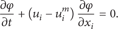
In order to simulate the free surface, the fractional function of fluid volume φ is introduced,

φ = {\begin{cases} φ = 0, & in air \\ 0 < φ < 1, & in free surface \\ φ = 1, & in water \end{cases}

(2)

which follows the advection equation as follows:

\frac{\partial φ}{\partial t} + (u_{i} - u_{i}^{m}) \frac{\partial φ}{\partial x_{i}} = 0 .

(3)

In this work, the contour φ = 0.5 is used to describe the free surface. In the computations, the averaging density and viscosity are used,

ρ = φ ρ_{w} + (1 - φ) ρ_{a}, μ = φ μ_{w} + (1 - φ) μ_{a},

(4)

where the subscripts w and a represent the water and air phases, respectively, and ρ_w = 1.0 × 10³ kg/m³, μ_w = 1.0 × 10⁻³ kg/m s, ρ_a = 1.0 kg/m³, and μ_a = 1.48 × 10⁻⁵ kg/m s.

The governing equation (1) and free surface equation (3) are solved by the finite volume method (FVM) and pressure implicit with splitting of operators (PISO) algorithm [15]. The Euler method is used to discretize the time-dependent term. The convection term and diffusion term are discretized by the Gauss limited linear method and the Gauss linear corrected method, respectively. The lumped-mass strategy is adopted to solve the linear system associated with the velocity unknowns while the BI-CGSTAB iteration is employed for the Poisson-type pressure equation.

The time step is automatically determined according to the CFL condition; that is,

Δ t < Cr \times \min {\frac{\sqrt{S_{e}}}{| u_{e} |}},

(5)

where Cr can be interpreted as the Courant number and S_e and u_e are the cell area and velocity, respectively. Some numerical tests show that Cr = 0.5 can guarantee the numerical stability and produce good accuracy. However, in order to simulate the transient impulsive pressure well, the much smaller time steps with Cr = 0.1 and Δt_max = 0.001 s are employed.

On the tank wall, the nonslip velocity boundary condition and the Neumann pressure boundary condition are imposed,

\begin{matrix} u_{i} = U_{i}, \\ \frac{\partial p}{\partial n} = 0, \end{matrix}

(6)

where U_i is velocity of tank wall due to external excitations. It should be noted that a zero referencing pressure is forced at the center of the tank ceiling.

3. Numerical Results

3.1. Two-Dimensional Results

A partially filled rectangular tank (Figure 1) with length B = 0.57 m, height H = 0.30 m, and liquid depth h = 0.15 m is considered. The lowest natural frequency is ω₁ = 6.0578 rad/s. The pressure probe P2 is situated at the still water level on the left wall and P4 is located at the left-up corner of the tank. The other four probes are placed close to P2 and P4 with a distance of 0.01 m. The tank is subjected to a forced sinusoidal horizontal excitation,

x (t) = x_{0} \sin ω t,

(7)

where the amplitude x₀ = 0.005 m and angular frequency ω = ω₁ are used. Three meshes Tabulated in table 1 are employed for mesh convergence test. As shown in Figure 2, convergent results can be obtained for Mesh 2 and Mesh 3. In present work, the Mesh 2 is used for simulation.

Table 1:

Mesh schemes for convergence test.

Mesh 1	Mesh 2	Mesh 3

9120	17984	26430

Figure 1:

Geometry setup of liquid sloshing in a rectangular tank.

Figure 2:

Mesh convergence test for free surface evolutions along the left wall of the tank with B = 0.57 m, H = 0.30 m, h = 0.15 m, x₀ = 0.005 m, and ω = 1.0ω₁.

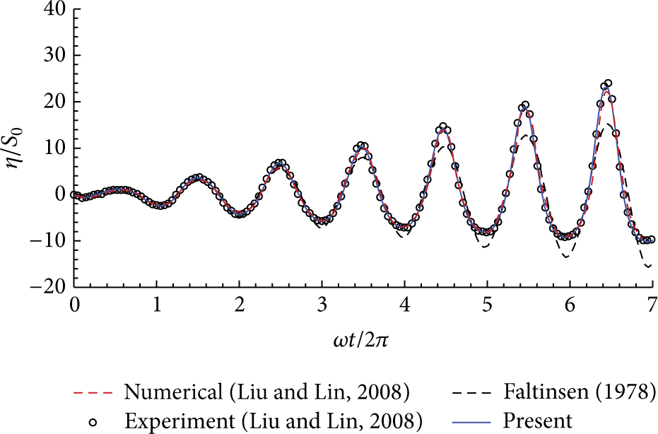
The present results of free surface elevation along the left wall are compared with the linear analytical solution by Faltinsen [1]; numerical and experimental results of Liu and Lin [14] are presented in Figure 3. The asymmetrical evolution of free surface elevation with time can be observed. This is due to the strong nonlinear effect under resonant excitation. At t = 7.2 s, the free surface runs up to the tank ceiling and the wave-breaking happens, which gives rise to the local irregular oscillation of free surface at wave trough. It can be seen from Figure 3 that the present numerical results agree well with the numerical and experimental results of Liu and Lin [14], indicating the good accuracy of the present model.

Figure 3:

Free surface evolutions along the left wall of the tank with B = 0.57 m, H = 0.30 m, h = 0.15 m, x₀ = 0.005 m, and ω = 1.0ω₁.

The evolutions of pressure at P1, P2, and P3 under the present resonant excitation are explained in Figure 4. The double-peak variations of pressure with time can be observed clearly from t = 5 s. With the elapse of time, the impulsive loads become more evident, especially at the first pressure peaks. The impulsive phenomenon near still water level is due to the hydraulic jump during the fluid oscillation [16]. The pressure signals reveal clear periodic impact pattern, but each impact pattern has different peak values. At P3, the maximum impulsive load is 1.103 kPa, more than 11.26 times of the local static pressure (0.098 kPa). At P1 and P2, the maximal values of impulsive pressure are 0.991 kPa and 1.044 kPa, respectively.

Figure 4:

Pressure signals at P1, P2, and P3 in the tank with B = 0.57 m, H = 0.30 m, h = 0.15 m, x₀ = 0.005 m, and ω = 1.0ω₁.

The dependence on the free surface variation of the impact pressure is explained in Figure 5, in which the nondimensional pressure p/p_max at the typical sampling point P2 and the free surface elevation η/η_max along the left wall are considered. The parameters p_max and η_max are 1.044 kPa and 0.15 m, respectively. As shown in Figure 5(a), the overall variation of the pressure at P2 is consistent well with the water level along the left wall. It means that the impact pressure is related closely to the free surface oscillation. If the wave amplitude is less than H − h (t < 7.2 s), for example, in Figure 5(b), the first and second pressure peaks correspond to the rising and falling stages of the free surface along the left wall, respectively. The minimum pressure at P2 is observed to happen at the instance with the highest water level. For t > 7.2 s, namely, the liquid runs up to tank ceiling and the first pressure peak appears before the free surface impacts the tank ceiling, as in Figure 5(c). And then, the pressure decreases and reaches minimum as the free surface attacks the tank ceiling. When the water level along the left wall sets down, the pressure at P2 rises up again, giving rise to the second peak value.

Figure 5:

Comparison of evolutions between pressure at P2 and free surface along left wall of the tank with B = 0.57 m, H = 0.30 m, h = 0.15 m, x₀ = 0.005 m, and ω = 1.0ω₁.

The time-series of pressure signals at P4, P5, and P6 under the resonant excitation are illustrated in Figure 6. The numerical results also show the impulsive phenomenon. By comparing the time-series of pressure, it seems that the impact processes at P4, P5, and P6 have the similar behavior. During the total period of 60 s, there are 7 impulsive loads greater than 1.2 kPa and one impulsive load greater than 1.8 kPa for both P5 and P6. The maximal impulsive loads are 2.14 kPa at P5 and 1.86 kPa at P6, respectively, happening at the same time of instant t = 58.08 s. However, the impact pressure at P4 is observed to be much larger than those of P5 and P6. There are 16 and 8 impulsive loads greater than 1.2 kPa and 1.8 kPa, respectively. The maximal impulsive pressure of P4 is 2.58 kPa at t = 11.33 s. These comparisons indicate that the tank ceiling corner is subjected to much more dangerous impact load under the resonant situation than its neighboring positions even with a small distance of 1 cm.

Figure 6:

Pressure signals at P4, P5, and P6 of the tank with B = 0.57 m, H = 0.30 m, h = 0.15 m, x₀ = 0.005 m, and ω = 1.0ω₁.

3.2. Three-Dimensional Results

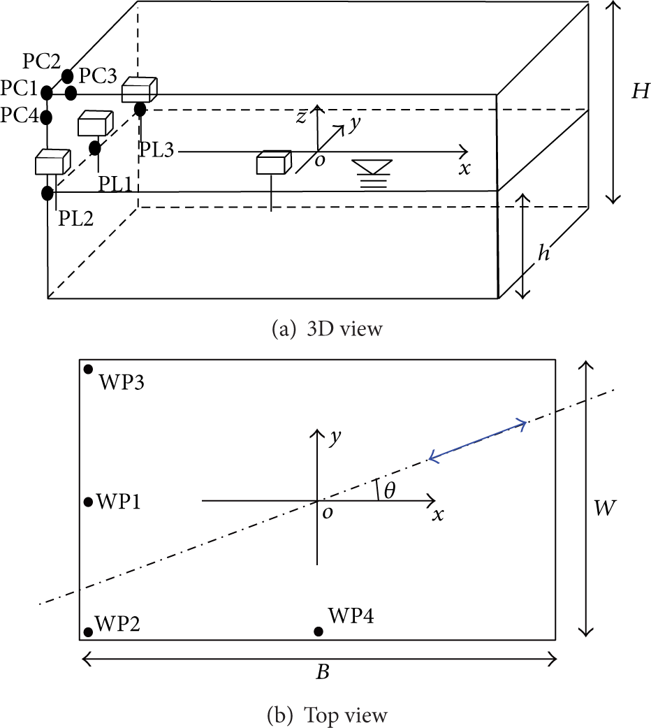
In Figure 7, the 3D rectangular tank with length B = 0.57 m, width W = 0.31 m, height H = 0.30 m, and liquid depth h = 0.15 m is considered. The lowest sloshing natural frequencies are ω₁₀ = 6.0578 rad/s (x-direction) and ω₀₁ = 9.5048 rad/s (y-direction). The sampling points of wave probes WP1 (−0.285, 0), WP2 (−0.285, −0.155), WP3 (−0.285, 0.155), and WP4 (0, −0.155) and pressure probes PL1, PL2, PL3, PC1, PC2, PC3, and PC4 are shown in Figure 7. The coordinates of the pressure probes are listed in Table 2.

Table 2:

Coordinates of pressure probes.

Probe	x (m)	y (m)	z (m)

PL1	−0.285	0	0
PL2	−0.285	−0.155	0
PL3	−0.285	0.155	0
PC1	−0.285	−0.155	0.150
PC2	−0.275	−0.155	0.150
PC3	−0.285	−0.145	0.150
PC4	−0.285	−0.155	0.140

Figure 7:

Geometric set-up of 3D sloshing.

The external excitation is assumed to follow a sinusoidal oscillation in horizontal plane, but with an angle θ with respect to the x-axis, referring to Figure 6(b). The components of the excitation in x- and y-axis are

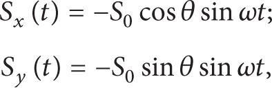
\begin{matrix} S_{x} (t) = - S_{0} \cos θ \sin ω t; \\ S_{y} (t) = - S_{0} \sin θ \sin ω t, \end{matrix}

(8)

where S₀ = 0.005 m, ω = 0.985ω₁₀ = 0.628ω₀₁ = 5.967 rad/s, and θ = 30°. The normalized free surface elevations at WP1 by the present numerical model and previous available data are compared in Figure 8. With the development of 3D sloshing, the difference between the present result and the linear solution by Faltinsen [1] can be identified. This is because the analytical solution cannot consider well the nonlinear effects involved in the near-resonant 3D sloshing. The accuracy of the present numerical results is confirmed by the good agreement with the numerical and experimental data of Liu and Lin [14].

Figure 8:

Comparisons of free surface elevations at WP1 for 3D tank with B = 0.57 m, W = 0.31 m, H = 0.30 m, h = 0.15 m, S₀ = 0.005 m, ω = 0.985ω₁₀, and θ = 30°.

The evolutions of free surface at three typical sampling points are compared in Figure 9. It can be seen that the sloshing amplitude at WP1 increases rapidly under the sustaining external excitation, accounting for the fact that the present exciting frequency is close to the natural frequency ω₁₀ for x-direction. The similar phenomenon can be observed also at WP2. Moreover, the much lower trough level at WP2 is observed in comparison with WP1. It implies that the more violent fluid resonance may appear at the tank corners due to the sharp configuration and the 3D effects. The wave amplitude at WP4, however, is rather limited.

Figure 9:

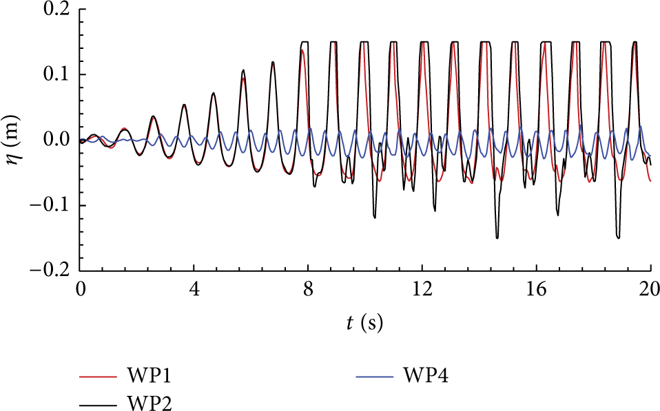
Free surface evolutions at WP1, WP2, and WP4 with B = 0.57 m, W = 0.31 m, H = 0.30 m, h = 0.15 m, S₀ = 0.005 m, ω = 0.985ω₁₀, and θ = 30°.

The time-series of pressure signals at the four probes of PC1, PC2, PC3, and PC4 are examined in Figure 10. And the corresponding statistical data are listed in Table 3. It can be seen from the figure that the fluid impact almost takes place at the same time for the four different sampling points. According to the data in Table 3, the smallest impulsive loads are observed at PC4. The peak values of PC2 and PC3 are close to each other. The largest impulsive pressure occurs at PC1, the corner of the tank ceiling.

Table 3:

Statistical analysis of pressure at PC1, PC2, PC3, and PC4 in the rectangular tank with B = 0.57 m, W = 0.31 m, H = 0.30 m, h = 0.15 m, S₀ = 0.005 m, ω = 0.985ω₁₀, and θ = 30°.

Probe	≥ 1.5 kPa	≥ 3.0 kPa	≥ 4.5 kPa	Maximal impulsive pressure (kPa)

PC1	19	8	1	5.28
PC2	18	7	0	4.01
PC3	18	5	0	3.57
PC4	16	0	0	2.67

Figure 10:

Pressure signals at PC1, PC2, PC3, and PC4 for the tank with B = 0.57 m, W = 0.31 m, H = 0.30 m, h = 0.15 m, S₀ = 0.005 m, ω = 0.985ω₁₀, and θ = 30°.

Considering again the above 3D tank but with θ = 0° for the external excitation oscillating, this allows the sloshing in the 3D tank to degrade to the 2D problem. The free surface elevations at WP1, WP2, and WP3 are compared in Figure 11. Similar phenomena such as the rapid increase and large amplitude of free surface oscillations can be observed with the 2D tank as in Figure 3. As the wave amplitude is less than H − h, not attacking the tank ceiling, the time histories of free surface logged by the three probes are in complete superposition. When the water runs up to the tank ceiling the noticeable difference between them can be observed; that is, the trough levels at WP2 and WP3 are much lower than that of WP1. It indicates that the more violent fluid motion happens at the tank corners due to the 3D effects of local sharp configuration. In addition, the free surface evolution still has evidence of discrepancy at WP2 and WP3, especially during the wave trough.

Figure 11:

Free surface evolution at WP1, WP2, and WP3 with B = 0.57 m, W = 0.31 m, H = 0.30 m, h = 0.15 m, S₀ = 0.005 m, ω = 0.985ω₁₀, and θ = 0°.

The evolutions of impact pressure at PL1, PL2, and PL3 are shown in Figure 13. The double-peak impulsive load can be observed. The overall variation of pressure is consistent well with the free surface oscillation in Figure 10, indicating that there is a close relationship between the impact pressure and local free surface elevation. Due to the 3D effect and nonlinearity, the pressure signals at the three probes are different from each other. The maximal impulsive loads are 0.917 kPa, 0.925 kPa, and 0.863 kPa during the process of 15 s at PL1, PL2, and PL3, respectively. They are close to that of the 2D tank in Figure 4 (1.044 kPa at P2). This indicates that the 2D model can work well in terms of the impact pressure near still water level as θ = 0°.

The time-series of pressure signals at PC1, PC2, PC3, and PC4 under the present near-resonant excitation are explained in Figure 12 and the statistical data are shown in Table 4. Because the four points are close to each other, the fluid impact almost takes place at the same instance as shown in Figure 12. From Table 4, the impact pressure at PC1 and PC3 is evidently larger than those of PC2 and PC4. Compared with the results in Table 3, the maximum impulsive pressure at PC1 for θ = 0° is slightly smaller than that of θ = 30°. Moreover, the impulsive load of probe P4 at the corner of 2D tank in Figure 5 is evidently smaller than that of the probe PC1 in the 3D tank. The maximum pressure at P4 is 2.58 kPa, while it is 4.51 kPa and 5.28 kPa at PC1 for θ = 0° and θ = 30°, respectively. This indicates that the 2D model may underestimate the impulsive pressure at the corner of tank ceiling comparing with 3D numerical model.

Table 4:

Statistical pressure at PC1, PC2, PC3, and PC4 in the rectangular tank with B = 0.57 m, W = 0.31 m, H = 0.30 m, h = 0.15 m, S₀ = 0.005 m, ω = 0.985ω₁₀, and θ = 0°.

Probe	≥ 1.5 kPa	≥ 3.0 kPa	≥ 4.5 kPa	Maximal impulsive pressure (kPa)

PC1	21	6	1	4.51
PC2	13	4	0	3.95
PC3	21	6	1	4.48
PC4	11	1	0	3.13

Figure 12:

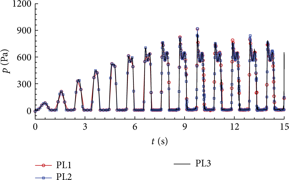
Pressure signals at PL1, PL2, and PL3 for the case with B = 0.57 m, W = 0.31 m, H = 0.30 m, h = 0.15 m, S₀ = 0.005 m, ω = 0.985ω₁₀, and θ = 0°.

Figure 13:

Pressure signals at PC1, PC2, PC3, and PC4 for the case with B = 0.57 m, W = 0.31 m, H = 0.30 m, h = 0.15 m, S₀ = 0.005 m, ω = 0.985ω₁₀, and θ = 0°.

4. Conclusion

The two- and three-dimensional liquid sloshing problem around the resonant condition is simulated by using the viscous fluid model OpenFOAM. The numerical validations show that the present numerical model works well in predicting the fluid motion under resonant excitation. Good agreements with available theoretical, numerical, and experimental results are obtained.

The numerical results in both 2D and 3D tank confirmed that the impulsive load, characterized by the local pressure around the still water level along the sidewall, consists of two peak values. The first peak value is observed as the free surface runs up toward the tank ceiling while the second appears as the free surface sets down. The relatively small pressure happens as the free surface attacks the tank ceiling.

The 3D numerical results show that the violent free surface motion and extremely large impact loads take place at the sharp corners. The 2D numerical model can produce accurate results in terms of the impact pressure near the still water level as the 3D tank undergoes 2D excitation with θ = 0°. Otherwise, it may remarkably underestimate the impulsive load comparing with 3D model, especially for the tank ceiling corners.

Conflict of Interests

The authors declare that there is no conflict of interests regarding the publication of this paper.

Footnotes

Acknowledgments

This work is supported by the National Natural Science Foundation of China (NSFC) with Grant no. 51109187 and the Zhejiang “Climbing Program” (pd2013217).

References

Faltinsen

O. M.

, “A numerical nonlinear method of sloshing in tanks with two-dimensional flow,” Journal of Ship Research, vol. 22, no. 3, pp. 193–202, 1978.

Nakayama

and Washizu

, “The boundary element method applied to the analysis of two-dimensional nonlinear sloshing problems,” International Journal for Numerical Methods in Engineering, vol. 17, no. 11, pp. 1631–1646, 1981.

Gedikli

and Ergüven

M. E.

, “Evaluation of sloshing problem by variational boundary element method,” Engineering Analysis with Boundary Elements, vol. 27, no. 9, pp. 935–943, 2003.

Nakayama

and Washizu

, “Nonlinear analysis of liquid motion in a container subjected to forced pitching oscillation,” International Journal for Numerical Methods in Engineering, vol. 15, no. 8, pp. 1207–1220, 1980.

Cho

J. R.

and Lee

H. W.

, “Non-linear finite element analysis of large amplitute sloshing flow in two-dimensional tank,” International Journal for Numerical Methods in Engineering, vol. 61, no. 4, pp. 514–531, 2004.

Wang

C. Z.

and Khoo

B. C.

, “Finite element analysis of two-dimensional nonlinear sloshing problems in random excitations,” Ocean Engineering, vol. 32, no. 2, pp. 107–133, 2005.

Celebi

M. S.

and Akyildiz

, “Nonlinear modeling of liquid sloshing in a moving rectangular tank,” Ocean Engineering, vol. 29, no. 12, pp. 1527–1553, 2002.

G. X.

Q. W.

, and Eatock Taylor

, “Numerical simulation of sloshing waves in a 3D tank based on a finite element method,” Applied Ocean Research, vol. 20, no. 6, pp. 337–355, 1998.

Armenio

and La Rocca

, “On the analysis of sloshing of water in rectangular containers: numerical study and experimental validation,” Ocean Engineering, vol. 23, no. 8, pp. 705–739, 1996.

10.

Chen

B.-F.

, “Viscous fluid in tank under coupled surge, heave, and pitch motions,” Journal of Waterway, Port, Coastal and Ocean Engineering, vol. 131, no. 5, pp. 239–256, 2005.

11.

Chen

B.-F.

and Nokes

, “Time-independent finite difference analysis of fully non-linear and viscous fluid sloshing in a rectangular tank,” Journal of Computational Physics, vol. 209, pp. 47–81, 2005.

12.

Kim

, “Numerical simulation of sloshing flows with impact load,” Applied Ocean Research, vol. 23, no. 1, pp. 53–62, 2001.

13.

Kim

Shin

Y.-S.

, and Lee

K. H.

, “Numerical study on slosh-induced impact pressures on three-dimensional prismatic tanks,” Applied Ocean Research, vol. 26, no. 5, pp. 213–226, 2004.

14.

Liu

D. M.

and Lin

P. Z.

, “A numerical study of three-dimensional liquid sloshing in tanks,” Journal of Computational Physics, vol. 227, no. 8, pp. 3921–3939, 2008.

15.

Issa

R. I.

, “Solution of the implicitly discretised fluid flow equations by operator-splitting,” Journal of Computational Physics, vol. 62, no. 1, pp. 40–65, 1986.

16.

Abramson

R. L.

Bass