
Abstract
A lot of mechanical parts are subject to failure due to the deterioration. Usually the preventive maintenance is taken to ensure the safety and reliability. Therefore, it is very important to study the gradual reliability design of the mechanical part for improving the gradual reliability of the mechanical system under the condition of considering the preventive maintenance. Beta distribution is employed to describe the randomness of the mechanical part state after the preventive maintenance. The deterioration process of the mechanical part is modeled using the nonstationary Gamma process. The gradual reliability model before the first preventive maintenance is proposed according to the gradual failure principle and using the initial state distribution and the properties of Gamma process. Then, the gradual reliability model between any two times of preventive maintenance is also derived. Subsequently, the sensitivity equations of the proposed gradual reliability model to each parameter are given. The application process and practicality of the proposed approach are described by a numerical example. This work solved the problem where the maintenance has not been well considered in the reliability design of the mechanical part and contributed to the theory and method of improving the safety and reliability operation of the mechanical system.
1. Introduction
Usually, most failures of mechanical equipment occur because some parameters deteriorate to a certain threshold. The deterioration factors mainly include wear, corrosion, fatigue, and creep. According to incomplete statistics, 80% of the mechanical part's failures are caused by wear [1]. Therefore, it is very important to protect the mechanical equipment from the type of failure for the safety production, cost reduction, availability improvement, and so on. It is objective of the gradual reliability analysis. Gradual reliability deals with the probability that the gradual failure of a device due to deterioration will not occur during a specified period of time under stated conditions.
Nowadays, the reliability calculation method is the focus of the reported literatures on gradual reliability. It might be classified into two types. One is the first crossing method where the times of the generalized stress crossing the generalized strength are stochastic and usually follow Poisson distribution. It has been applied to many engineering examples, such as [2–7]. The another one is to transform the gradual reliability into static one where there are only random variables and there is no stochastic process. The considered time t is discretized into t0 = 0, t1, t2,…, t N = t. The generalized stress X(t) and strength S(t) which are stochastic processes are dispersed by the same time interval. X i and S i which are the discrete generalized stress and strength between ti − 1 and t i are assumed as random variables. Then the gradual reliability could be calculated by a lot of static reliability calculation methods. The method has been discussed by many researchers, such as [8–12]. The gradual reliability estimation, where the strength was constant and the mechanical part was suffered from n random stresses following the same distribution during a period of time, has been discussed in [13–16]. n random stresses were replaced by an equivalent stochastic variable and n was assumed to be Possion process. Then, the gradual reliability was estimated by the static reliability calculation method. The another especial gradual reliability was solved by the static method. Here, the state function was a monotone decreasing function and the static reliability at t time was equal to the corresponding gradual reliability [17]. Moreover, the gradual reliability calculation method based on Gamma process has been presented by the author and applied to the cutting tool reliability design of CNC machine tools in [18, 19].
The gradual reliability considering the preventive maintenance action has been discussed by some literatures, such as [20, 21], where the preventive maintenance action was supposed to renew the mechanical part. In this work, the imperfect preventive maintenance is discussed in the gradual reliability sensitivity analysis. The remainder is organized as follows: the gradual reliability model considering a preventive maintenance action and its sensitivity analysis are derived in Sections 2 and 3; the numerical examples are given in Section 4; and the conclusions are drawn finally.
2. Gradual Reliability Model considering Preventive Maintenance
2.1. Preventive Maintenance and Mechanical Part Deterioration Model
The imperfect preventive maintenance has been formulated by many documents. The achievements were reviewed in [22, 23]. Two models are well-known. One is virtual age model proposed by Kijima. The lift span of mechanical part was decreased after a preventive maintenance action [24]. Another One is Brown-Proschan model. After a preventive maintenance, the probability of refreshing the mechanical part state to the new one is p (0⩽p⩽1) and 1 − p is the probability of the mechanical part keeping the state before the maintenance. In this work, the preventive maintenance is described by the model which was proposed in [25] and extended Brown-Proschan model. The mechanical part state is stochastic and follows Beta distribution after the mechanical part is maintained; that is,

where
The main deterioration factors of the mechanical part are composed of wear, corrosion, fatigue and creep, and so forth in general. The deterioration process is a continuous-time and continuous-state stochastic process. Moreover, it is also a monotone increasing or decreasing stochastic process. Therefore, the Gamma process is employed to describe the mechanical part deterioration. A Gamma process is a stochastic process with the independent, nonnegative increment having a Gamma distribution with an identical scale parameter. It is a continuous-time and continuous-state stochastic process. Let {X1(t), t ≥ 0} be a Gamma process with the following properties [26]:
X1(0) = 0 with probability one,
X1(τ) − X1(t)~G(x ∣ v(τ) − v(t),u), ∀τ > t ≥ 0,
X1(t) has independent increments,
where G(·) is the Gamma distribution and its probability density function is

v(t) is the shape function which is a non-decreasing, right-continuous, real-valued function for t ≥ 0 with v(0)≡0, and u > 0 is the scale parameter. Empirical studies show that the expected deterioration at time t is often proportional to a power law [26], that is E(X1(t) − X1(0)) = ct b /u = at b ∝t b , where a > 0 (or c > 0) and b > 0.
2.2. Gradual Reliability Model considering Preventive Maintenance
DF is defined as the gradual failure threshold of the mechanical part and is determined by the design requirement or engineer. According to the principle that the mechanical part state is not more than DF, the gradual state function of the mechanical part with considering the preventive maintenance is
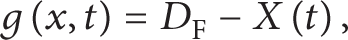
where X(t) = X0(0) + ΔX1(t). X0(0) is the initial random state variable and is

and h0 is the determinate design value. h is the random actual one. It follows the normal distribution generally. X1(t) is the random deterioration variable at t time. According to the definition of Gamma process, ΔX1(t)≡X1(t) − X1(0). Then, X(t) = X0(0) + (X1(t) − X1(0)), where X1(t) − X1(0) follows Gamma distribution.
To clarify the gradual state function, the length deterioration failure of a rod due to wear is introduced. The determinate design length is h0. The actual length h is generally a random variable with the mean h0 because the machining processes are affected by a lot of stochastic factors, such as manufacturing accuracy of machine tool, ambient temperature, random fluctuating of motor speed, and material uniformity. Then, X0(0) is a random variable with the mean 0. At time 0, the wear X1(0) = 0 with probability one. The wear length is zero and the gradual reliability is equal to the probability of the wear threshold DF which is not less than X0(0). At time t, the wear length is X1(t) and the probability of DF⩾X0(0) + ΔX1(t) is the gradual reliability of the rod.
t1 is defined as the time when the first preventive maintenance action is triggered. When t⩽t1, the gradual reliability could be calculated by

where X0(0) and X1(t) are considered to be independent and
t1+ and t2 are assumed to be the end time of the first preventive maintenance and the time of triggering the second preventive maintenance action, respectively. When t1+⩽t⩽t2, the mechanical part state is determined by both the initial random variable X0(t1+) and the deterioration increment X1(t1′) − X1(t1). Here, t1′ = t − T1 and T1 = t1+ − t1. T1 are the period for implementing the first preventive maintenance action. Then, the mechanical part state is

The gradual reliability (t1+⩽t⩽t2) is

where DPM is the preventive maintenance threshold and X0(t1+) and X1(t1′) − X1(t1) are also assumed to be independent.
In the same way, the mechanical part state (t i +⩽t⩽ti + 1) is

where t i + and ti + 1 are the end time of the ith preventive maintenance and the starting time of the (i + 1) th preventive maintenance action and t i ′ = t − ∑j = 1 i T j . T j is the period for implementing the ith preventive maintenance. The corresponding gradual reliability is obtained by substituting (8) into (7).
3. Gradual Reliability Sensitivity Analysis
In order that the effect of each parameter on the gradual reliability of mechanical part can be distinguished and more sensitive parameters can be controlled strictly in the design, the gradual reliability sensitivity is analyzed in this section. Using the derivation theorem, the sensitivity of the gradual reliability R1(t) to the gradual failure threshold DF and deterioration process parameters c, b, and u, respectively, are

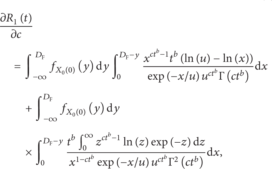


where
The sensitivity of Ri + 1(t) to the parameters c, b, and u could be computed by (10), (11), and (12), respectively. The respective sensitivity of Ri + 1(t) to DF, DPM, α i , and β i are

where
4. Numerical Analysis
How to apply the presented gradual reliability sensitivity method to improve the mechanical part reliability should be shown by the numerical example in the section. Here the Gamma process parameters are c = 1.5, b = 2.0, and u = 3. The initial random state variable X0(0) follows the normal distribution in which the mean and variance are zero and 0.03. The gradual failure threshold DF = 5.0. The preventive maintenance threshold DPM= 4.5. The number of the preventive maintenance is supposed to be 3 and the parameters of the preventive maintenance model are α1 = 2, β1 = 2, α2 = 3, β2 = 2, α3 = 5, and β3 = 2.
The gradual reliability curve is shown in Figure 1. When the preventive maintenance is not operated, the reliability R1(t) curve is the left one in Figure 1. It could be seen that the gradual reliability of the considered mechanical part could be improved by the preventive maintenance greatly and its decreasing velocity is faster and faster with the increasing number of the preventive maintenance actions as in Figure 1.

Gradual reliability curve considering preventive maintenance of mechanical part.
The sensitivity curve of the gradual reliability of the numerical example to the Gamma process parameters b, c, and u, the gradual failure threshold DF, the parameters of the preventive maintenance model α and β, and the preventive maintenance threshold DPM are shown in Figures 2, 3, 4, 5, 6, 7, and 8, respectively. According to Figures 2–8, it is shown that the sensitivity to b, c, u, α, and DPM almost is equal or less than zero and that to DF and β is more than zero. Therefore, the gradual reliability of the mechanical part in the numerical example could be improved by decreasing the parameters b, c, u, α, and DPM and increasing DF and β. It means to slow the wear, reduce the preventive maintenance threshold, increase the gradual failure threshold, and improve the maintenance quality.

Sensitivity curve of gradual reliability R(t) to Gamma process parameter b.

Sensitivity curve of gradual reliability R(t) to Gamma process parameter c.

Sensitivity curve of gradual reliability R(t) to Gamma process parameter u.

Sensitivity curve of gradual reliability R(t) to gradual failure threshold DF.

Sensitivity curve of gradual reliability R(t) to preventive maintenance model parameter β.

Sensitivity curve of gradual reliability R(t) to preventive maintenance model parameter α.

Sensitivity curve of gradual reliability R(t) to preventive maintenance threshold DPM.
5. Conclusion
The gradual reliability model of the mechanical part considering preventive maintenance was formulated and its sensitivity was given. The numerical example was analyzed to illustrate how to improve the gradual reliability of the mechanical part suffered from the preventive maintenance by the proposed method.
Conflict of Interests
The authors declare that there is no conflict of interests regarding the publication of this paper.
Footnotes
Acknowledgments
The work is supported by Chinese National Natural Science Foundation (Grant no. 51135003), Major State Basic Research Development Program of China (973 program) (Grant no. 2014CB046303), and New Century Excellent Talents Support Plan of China Ministry of Education (Grant no. NCET-12-0105).