Application of Modal Parameter Estimation Methods for Continuous Wavelet Transform-Based Damage Detection for Beam-Like Structures

Abstract

This paper presents a hybrid damage detection method based on continuous wavelet transform (CWT) and modal parameter identification techniques for beam-like structures. First, two kinds of mode shape estimation methods, herein referred to as the quadrature peaks picking (QPP) and rational fraction polynomial (RFP) methods, are used to identify the first four mode shapes of an intact beam-like structure based on the hammer/accelerometer modal experiment. The results are compared and validated using a numerical simulation with ABAQUS software. In order to determine the damage detection effectiveness between the QPP-based method and the RFP-based method when applying the CWT technique, the first two mode shapes calculated by the QPP and RFP methods are analyzed using CWT. The experiment, performed on different damage scenarios involving beam-like structures, shows that, due to the outstanding advantage of the denoising characteristic of the RFP-based (RFP-CWT) technique, the RFP-CWT method gives a clearer indication of the damage location than the conventionally used QPP-based (QPP-CWT) method. Finally, an overall evaluation of the damage detection is outlined, as the identification results suggest that the newly proposed RFP-CWT method is accurate and reliable in terms of detection of damage locations on beam-like structures.

1. Introduction

Cracks within a structure due to the material fatigue result in serious threats to property security. Therefore, early crack detection is important and necessary. An effective and reliable crack detection technique has been sought by corporations that utilize no-destructive testing (NDT) or structural healthy monitoring (SHM), and such a detection technique has been the subject of research in various related fields [1]. The related literature over the past two decades has introduced extensive methods for damage detection, focusing on crack or damage detection based on changes in the modal parameters [2–4].

Modal analysis is a strong and reliable vibration analysis tool used in modern engineering. Any crack or damage that exists will induce mode changes; for example, the natural frequency will decrease, damping will be added, and mode shapes will be altered. Owolabi et al. [5] successfully used the changes in the natural frequencies and amplitudes of the frequency response function (FRF) to detect cracks in beams. Different detection methods based on natural frequencies were also reviewed by Salawu [6]. However, crack detection methods using frequencies can only provide a global judgment, as they lack local information. Currently, due to the spatial property of mode shape, mode shape is more often used in damage detection. The advantage of mode shape and its derivative is that they are less influenced by their environment and are more sensitive to local damage [7]. To identify the damage in a beam, Ratcliffe [8] applied the finite difference Laplacian function to the mode shapes of damaged beams. Further postprocessing of the Laplacian function enables the identification of less severe damage, even for damage less than 0.5%. A postdoctoral program sponsored by NASA [9] proposed a mode-shape-based fault detection methodology for cantilever structures, such as the wing of an airplane. Elshafey and his partners [10] considered the normalized difference between the intact and damaged mode shapes as a virtual displacement at each node and added them to the coordinates of the original undeformed structure, thereby identifying the damaged location using the virtually deformed shape.

The wavelet transform (WT) is a relatively new technology that has, over the past two decades, developed quite rapidly. It has been widely utilized in many different kinds of fields [11, 12]. Due to its outstanding sensitivity to the singularities in signals, WT can identify abrupt changes occurring in mode shapes, which typically indicates damage to or cracks in a structure. Rucka [13] applied the CWT to the first eight mode shapes to check the effect of higher modes on damage to a cantilever beam. They claimed that high modes were able to more easily recognize the damage. Fan and Qiao [14] proposed a 2D CWT-based algorithm to identify the damage on plate structures. This method was applied to the numerical vibration mode shapes in a modal experiment, which proved the robustness of the algorithm. Zhong and Oyadiji [15] performed a CWT on two sets of mode shapes difference, which were derived from the reconstructed modal data of a cracked simply supported beam. Even though the results that were finally obtained were accurate, some modes were easily affected by experimental noise, making it difficult to confirm the correct crack position; therefore, a threshold for the wavelet coefficients had to be set to filter out the noise effect. Rucka and Wilde [16] applied the “Gaussian” wavelet and reverse “biorthogonal” wavelet to one-dimensional (1D) and two-dimensional (2D) structures, respectively. In their research, an integral damage detection method using the raw hammer/vibration data, based on the QPP method, was provided for a cantilever beam. Due to the interference of experimental noise, however, the identified error rate was up to 9.1%. In order to reduce the noise effect, a stationary wavelet transform (SWT) denoise procedure with a soft-thresholding was performed by Zhong and Oyadiji [17] on the modal data to remove the noise. Ovanesova and Suárez [18] applied the discrete wavelet transform (DWT) and CWT to the deflection responses occurring from dynamic and static loads, respectively. Their numerical results showed that the damage could be identified; however, the results were confused by the boundary conditions, especially for the CWT. They concluded that subsequent experimental tests needed to be performed, as a real-world application could not be estimated only depending on numerical simulation.

As seen from previous researches, current CWT-based techniques for crack or damage detection methodology are effective and reliable. Furthermore, tangible experiments are indispensable in terms of their applications. In addition, the experimental noise should be given a significant amount of consideration, as it can affect the identification results. Furthermore, for the experimental noise effect, most of the previous studies focused on the postprocess of the mode shape or the coefficients of wavelet transform, with only a few studies emphasizing the methods of the mode shape estimation itself. However, any kinds of denoising approach on mode shape or wavelet coefficients, such as smoothing and threshold, will easily change the nature of signal, therefore, how to remove the noise fundamentally becoming extraordinarily important.

In this paper, a more reliable damage detection approach (RFP-CWT) is proposed. Our method is based on mode shape using a CWT technique. Due to the significant denoising ability of the improved version of RFP technique, the proposed hybrid damage detection method exhibited a better performance than the usually used QPP-based method. In view of application, the RFP-CWT can be directly used in the damage detection of beam-like structure in engineering.

2. Basic Theory

2.1. Frequency Response Function (FRF) and Mass-Normalized Mode Shape

According to the second law of Newton's or Lagrange's theory, a linear mechanical system for a multidegree of freedom (MDOF) can be expressed by

$\left[M\right]\left\{\ddot{x}\right\}+\left[C\right]\left\{\dot{x}\right\}+\left[K\right]\left\{x\right\}=\left\{f\left(t\right)\right\},$

(1)

where [M] is the inertia mass matrix, [C] is the damping coefficient matrix, [K] is the stiffness matrix, and f(t) is the external force. In the Laplace domain, (1) can be represented by

$\left(\left[M\right]s^{\mathrm{2}}+\left[c\right]s+\left[K\right]\right)\left\{X\left(s\right)\right\}=\left\{F\left(s\right)\right\}.$

(2)

Here, s = jω is the Laplace factor. Therefore the system transfer function can be inferred as

$\left[H\left(s\right)\right]=\frac{\mathrm{1}}{\left[M\right]s^{\mathrm{2}}+\left[c\right]s+\left[K\right]}=\frac{\left\{X\left(s\right)\right\}}{\left\{F\left(s\right)\right\}}.$

(3)

In the frequency domain, the transfer function is known as FRF given by

$\left[H\left(\omega \right)\right]=\frac{\left\{x\left(\omega \right)\right\}}{\left\{F\left(\omega \right)\right\}}.$

(4)

Mode shapes of a system are unique in terms of their shapes, but not in terms of their values, as multiples of them can be equally valid. Mass-normalized mode shapes are unique presentations of the mode shapes. A mass-normalized mode shape comes from the normalization of a mode shape using the modal mass. Based on the relationship {Φ} _r ^T [M]{Φ} _r = m _r (r = 1,2, 3, …, n), the mode shape {Φ} _r can be normalized by

${\left\{\phi \right\}}_r=\frac{\mathrm{1}}{\sqrt{m_r}}{\left\{\Phi \right\}}_r\hspace{1em}\left(r=\mathrm{1},\mathrm{2},\mathrm{3},\dots ,n\right),$

(5)

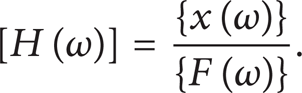
where {ϕ} _r is the rth mass-normalized mode shape of the system, which is unique to a multidegree of freedom (MDoF) system. The most important thing is that the FRF of an MDoF system can be described by a mass-normalized mode shape and natural frequencies; therefore, through a modal analysis, the mass-normalized mode shape is obtainable. A single FRF can be defined as [19]

$H_{jk}\left(w\right)=\left\{A_{jk}^r\right\}\left\{\frac{\mathrm{1}}{{\lambda }_r^{\mathrm{2}}-w^{\mathrm{2}}}\right\},$

(6)

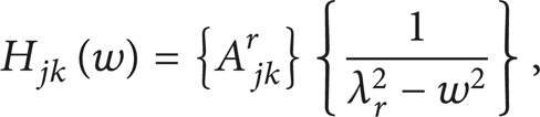
where A _jk ^r = ϕ _jr ϕ _kr is the modal constant of the FRF between the response point j and excitation point k. The lth row of FRF-matrix can be written as

${\left[H\left(w\right)\right]}_l=\left[\begin{array}{cccc}{\alpha \left(w\right)}_{l\mathrm{1}}& {\alpha \left(w\right)}_{l\mathrm{2}}& \cdots & {\alpha \left(w\right)}_{ln}\end{array}\right]=\left[A_l\right]\left\{\frac{\mathrm{1}}{{\lambda }_r^{\mathrm{2}}-w^{\mathrm{2}}}\right\},$

(7)

where

$\left[A_l\right]=\left[\begin{array}{cccc}{A}_{l\mathrm{1}}^{\mathrm{1}}& A_{l\mathrm{2}}^{\mathrm{1}}& \cdots & A_{ln}^{\mathrm{1}}\\ A_{l\mathrm{2}}^{\mathrm{2}}& A_{l\mathrm{2}}^{\mathrm{2}}& \cdots & A_{ln}^{\mathrm{2}}\\ \cdots & \cdots & \cdots & \cdots \\ A_{ln}^r& A_{ln}^r& \cdots & A_{ln}^r\end{array}\right]=\left[\begin{array}{cccc}{\phi }_{l\mathrm{1}}^{\mathrm{1}}{\phi }_{\mathrm{11}}^{\mathrm{1}}& {\phi }_{l\mathrm{1}}^{\mathrm{1}}{\phi }_{\mathrm{21}}^{\mathrm{1}}& \cdots & {\phi }_{l\mathrm{1}}^{\mathrm{1}}{\phi }_{n\mathrm{1}}^{\mathrm{1}}\\ {\phi }_{l\mathrm{2}}^{\mathrm{2}}{\phi }_{\mathrm{12}}^{\mathrm{2}}& {\phi }_{l\mathrm{2}}^{\mathrm{2}}{\phi }_{\mathrm{22}}^{\mathrm{2}}& \cdots & {\phi }_{l\mathrm{2}}^{\mathrm{2}}{\phi }_{n\mathrm{2}}^{\mathrm{2}}\\ \cdots & \cdots & \cdots & \cdots \\ {\phi }_{ln}^r{\phi }_{\mathrm{1}n}^r& {\phi }_{ln}^r{\phi }_{\mathrm{2}n}^r& \cdots & {\phi }_{ln}^r{\phi }_{nn}^r\end{array}\right],$

(8)

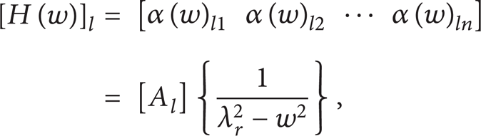
where r is number of spectrum lines, n is the number of DOFs of the structure, and matrix [A _l ] is the modal constant matrix for the lth rows of the FRF matrix, which is different from the residue. Based on the interrelationship between modal constant and mass-normalized mode shape, that is, A _jk ^r = ϕ _jr ϕ _kr , particularly, when j = k, the following equation can be determined:

$A_{jj}^r={\phi }_{jr}{\phi }_{jr}.$

(9)

This equation is known as the driving point measurement (DPM) method for the extraction of a mass-normalized mode shape. The driving point modal constants can be obtained by curve fitting of the corresponding FRF measurement. Moreover, when the driving point FRF is impossible to access or difficult to measure, the off-diagonal measurement can be used as an alternative. Further details can be found in [20].

2.2. Wavelet Transform

Over the past twenty years, the WT technique has become an extremely attractive signal processing tool and has been applied in various subfields, such as mathematics, science, and engineering. Through the scaling and translating of one original wavelet, known as the mother wavelet or basic wavelet, each subsequent wavelet, called the daughter wavelet, is produced. As such, a technique superior to the short time Fourier transform (STFT), which involves multiscale analysis of a signal, can be performed using a WT in the time and frequency domain (time-frequency domain). Consequently, the wavelet transform is more suitable for the analysis of nonstationary signals. Recently, the WT technique has been used successfully in machine fault diagnostics due to its analytical capabilities for nonstationary signals, among other reasons.

The function ψ(x) performs the operations of translation and dilatation to create a family of wavelets, ψ_{u, a}(x), formulated as

${\psi }_{u,a}\left(x\right)=\frac{\mathrm{1}}{\sqrt{a}}\psi \left(\frac{x-u}{a}\right),$

(10)

where the parameters u and a denote the translation and scale factors, respectively. In the time-frequency domain, parameter u shows the time variable, parameter a represents the shrinking or stretching of the wavelet function, and 1/a plays an equivalent role to Fourier frequency ω. Due to the outstanding adaptability of a wavelet, it provides a high time resolution for higher frequencies and a high-frequency resolution for lower frequencies.

Based on the idea of associating a given wavelet of scale a with a purely periodic signal of frequency ω, the relationship between scale factor a and pseudofrequency can be obtained by the following equation [21]:

$F_a=\frac{F_c}{a·\Delta },$

(11)

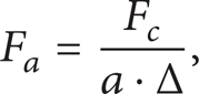
where F _a is the pseudofrequency corresponding to scale a, Δ represents the sampling period, and F _c is the center frequency of a wavelet.

The CWT of a function f(x) is the inner product of the signal function with the complex conjugate functions of a wavelet and is defined as follows [22]:

$W_f\left(a,u\right)=\frac{\mathrm{1}}{\sqrt{a}}{{\displaystyle \int }}_{-\infty }^{+\infty }f\left(x\right){\psi }^{*}\left(\frac{x-u}{a}\right)dx,$

(12)

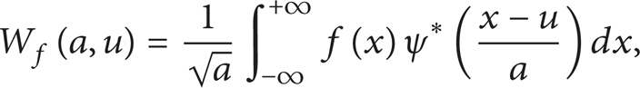
where a is the scale factor and u is the translation factor. ψ^* indicates the complex conjugate of the wavelet function, known as the wavelet coefficients. The CWT measures the similarity or correlation of the wavelet and the signal to be analyzed. If there is a higher similarity or correlation among them, the wavelet coefficients are bigger. Normally, the wavelet function ψ is an oscillatory function and a real or complex-valued function with a zero average and a finite length; that is, compact support:

${{\displaystyle \int }}_{-\infty }^{+\infty }\psi \left(x\right)dx=\mathrm{0}.$

(13)

Due to the characteristics of multiscale, scale-space attributes, and redundancy coefficients, CWT has the ability to detect subtle changes or singularities, like breakdown points or discontinuities in a signal, which also explains why CWT is usually superior to DWT in NDT [23]. An important property of a wavelet function is its vanishing moments. If a wavelet has n vanishing moments, it should be satisfied by the following condition:

${{\displaystyle \int }}_{-\infty }^{+\infty }{x}^k\psi \left(x\right)dx=\mathrm{0},\hspace{1em}k=\mathrm{0},\mathrm{1},\mathrm{2},\dots ,n-\mathrm{1}.$

(14)

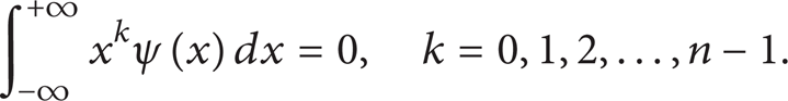
The proper selection of wavelet type and the chosen number of the vanishing moments will determine the sensitivity of changes induced by damage. The wavelet with an n vanishing moment indicates that the wavelet coefficients are zero for polynomials of a degree that is, at most, n − 1. In theory, more vanishing moments mean that the scaling function can represent more complex signals accurately. Conversely, the more vanishing moments there are, the worse the localized ability becomes, as Daubechies proved [24], indicating that the compromise between the number of vanishing moments and support length should be considered. Empirically, the number of vanishing moments is chosen as 2 or 4 [15, 16]. In this paper, after several pretests using various kinds of wavelets, like the Morlet wavelet, Symlets wavelet, and the Gaussian wavelet [21, 22], the Gaussian wavelet (gaus4), which has four vanishing moments, was finally selected as the best candidate for this study.

3. Experimental Procedure

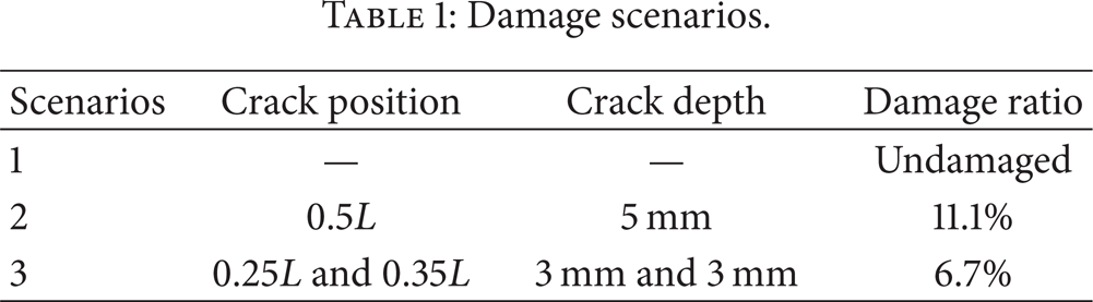
For application purposes, the component of a beam-like pin with light damping, which is commonly used in the subtrain, was selected as the test sample in this work. The experimental specimens consisted of three beams representing different damage level scenarios (Table 1). A free-free boundary condition was simulated by placing the pin on a porous foam pad, which guarantees the self-vibration frequency of the porous foam pad within ten percent of the lowest natural frequency of the tested beam. The diameter of the right-end cylinder of the beam (φ₂) was 45 mm and its length (L₂) was 325 mm. The diameter (φ₁) of the left-end disk-like component of the beam was 73 mm and its thickness (L₁) was 15 mm. The total length of the beam (L = L₁ + L₂) was 340 mm and the geometry shape for the intact one is shown in Figure 1. The elastic modulus of the beam (E) was 230 GPa, the density (ρ) was 6730 kg/m³, and Poisson's ratio was σ = 0.3.

Table 1:

Damage scenarios.

Scenarios	Crack position	Crack depth	Damage ratio
1	—	—	Undamaged
2	0.5L	5 mm	11.1%
3	0.25L and 0.35L	3 mm and 3 mm	6.7%

Figure 1:

Geometry of the intact beam-like pin.

An impact hammer, which is a fast and convenient way used in modal analysis to find the modes in a machine or structure, was employed to excite the components. In this study, by way of hand-tapping, 34 measurement points were selected with a sampling distance of 10 mm along the beam from the left-end of the cylinder. The used PCB 086C03 hammer with a sensitivity of 10 mV/lbf can provide a broad band excitation force to the structure while the vibration acceleration signals are measured at specified point. One accelerometer of the PCB model 353B14 piezoelectric with a frequency range of 0.7–18000 Hz and a sensitivity of 5 mV/g was arranged to capture the response signal by fixing one reference point. The reference point for the accelerometer was carefully selected. In principle, it should not be the nodal point and should be positioned such that all modes contribute to the point. Here, several pretests were performed to ensure the proper selection of the reference point. The impacts were repeated six times per measurement point to obtain the average values using a roving hammer, thus decreasing the disturbance of experimental noise. The experimental setup is shown in Figure 2.

Figure 2:

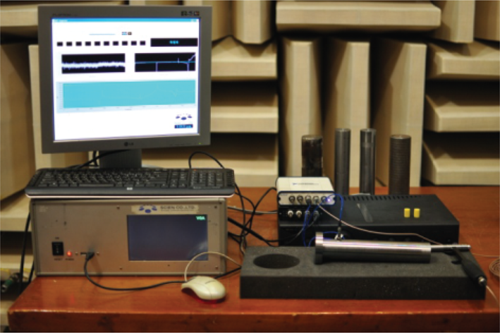
Experimental setup for modal analysis in the laboratory.

Based on the pretest and consideration of our frequency of interest, the maximum analytical frequency of the vibration response signal was determined to be approximately 6000 Hz. Therefore, the sampling rate of the data acquisition system was 16000 Hz, which satisfies the Nyquist-Shannon sampling theorem. The maximum number of samples was 16384 for a convenient calculation of the fast Fourier transform (FFT) providing an enough resolution. A Butterworth IIR low-pass filter was employed for both of the responses and the input (force) signal in order to avoid any aliasing induced by unwanted high-frequency components. The exponential and force windows were applied to acceleration response and force of the signal in order to prevent energy leakage before the FFT.

4. Mode Shape Estimation and Comparison

Curve fitting is the process of estimating the modal parameters using a mathematical approach to match the experimental measurements as accurately as possible. There are several classical curve fitting methods found in previous research [25], which can be classified into two types: that is, time domain and frequency domain. The most popular time domain method is the least-squares complex exponential (LSCE) [26, 27], which uses the Prony algorithm to curve-fit the impulse response. Unfortunately, this method causes time domain leakage or wrap around errors when taking the inverse Fourier transform from a set of FRF measurements. In the frequency domain, the easiest and fastest method is the QPP [28, 29], which takes the imaginary part peaks of the measured FRF as the mode shape factor to identify the mode shape. Another effective frequency domain curve fitting procedure is the RFP method. Compared to other frequency domain methods, the RFP method can be applied over any frequency range of data, especially in the vicinity of a resonance frequency [30]. Moreover, the RFP can provide accurate results, even if the measurements suffer from experimental noise. The second part of this chapter provides specific details concerning the RFP technique.

4.1. Mode Shape Determination by QPP Method

The mode shape factor is directly related to the mode shape, which is proportional to the modal coefficient and can be determined from the imaginary part of the FRF measurement. Figure 3 shows an example of the imaginary part of the FRF for a measure point (6, 12), which was obtained by measuring the response at Point 6 and the exciting force at Point 12 along a beam from the left-hand side. As Figure 3 illustrates, the imaginary part of the FRF reached a peak value at the natural frequency position. The mode shape factor can be taken as the value of the imaginary part of FRF at the position of resonance frequency, with the sign being in accordance with the peak lying along the imaginary axis. Accordingly, estimating the mode shape mathematically can be formulated as (15), where ϕ _i (i = 1, 2, …, n) represents the ith mode shape vector, H is the FRF vector, m is the mth response point, n is the nth impact point, ${\left\{H_{m,n}\right\}}^{\mathrm{1}\text{th}}$ represents the first mode that corresponds to the mth response point at the nth impact point, and the operator of “Amp” and “im” represents the amplitude and imaginary part of FRF, respectively. The mode shape at each resonance frequency can be illustrated by the mode shape factors for each measurement point along the beam. For brevity, only the first four mode shapes are given in Figure 5, shown as the blue circle-dash line:

$\left[\begin{array}{c}\begin{array}{c}{\mathit{\phi }}_{\mathrm{1}}\\ {\mathit{\phi }}_{\mathrm{2}}\\ ⋮\end{array}\\ {\mathit{\phi }}_n\end{array}\right]=\text{Amp}\left[\begin{array}{ccccc}\text{im}{\left\{H_{m,\mathrm{1}}\right\}}^{\mathrm{1}\text{th}}& \cdots & \text{im}{\left\{H_{m,k}\right\}}^{\mathrm{1}\text{th}}& \cdots & \text{im}{\left\{H_{m,n}\right\}}^{\mathrm{1}\text{th}}\\ \text{im}{\left\{H_{m,\mathrm{1}}\right\}}^{\mathrm{2}\text{th}}& \cdots & \text{im}{\left\{H_{m,k}\right\}}^{\mathrm{2}\text{th}}& \cdots & \text{im}{\left\{H_{m,n}\right\}}^{\mathrm{2}\text{th}}\\ ⋮& ⋮& ⋮& ⋮& ⋮\\ \text{im}{\left\{H_{m,\mathrm{1}}\right\}}^{n\text{th}}& \cdots & \text{im}{\left\{H_{m,k}\right\}}^{n\text{th}}& \cdots & \text{im}{\left\{H_{m,n}\right\}}^{n\text{th}}\end{array}\right].$

(15)

Figure 3:

Imaginary part of the FRF (H_6,12(ω)) matrix for the undamaged beam of Scenario 1.

4.2. Mode Shape Determination by RFP Method

The RFP method curve fits the FRF measurements to determine the coefficients of both the numerator and denominator polynomials, since the measurement FRFs can be represented by rational polynomials, as illustrated in the following equation, thereby identifying the system's characteristics:

$H\left(\omega \right)=\frac{{\sum }_{k=\mathrm{0}}^{\mathrm{2}N-\mathrm{1}}{a}_k{s}^k}{{\sum }_{k=\mathrm{0}}^{\mathrm{2}N}{b}_k{s}^k},\hspace{1em}s=j\omega ,$

(16)

where H(ω) is FRF, ω is the angular frequency, and a _k and b _k are the numerator and denominator of a rational fraction polynomial. To curve-fit the measured FRF, the error function for the ith single frequency bin can be written as

$e_i=\frac{{\sum }_{k=\mathrm{0}}^{\mathrm{2}N-\mathrm{1}}{a}_k{\left(j{\omega }_i\right)}^k}{{\sum }_{k=\mathrm{0}}^{\mathrm{2}N}{b}_k{\left(j{\omega }_i\right)}^k}-H_e\left({\omega }_i\right),$

(17)

where H _e (ω _i ) is the experiment FRF of the ith frequency bin. The error function can be linearized using a modified error function:

$e_i^{\prime }=e_i{\displaystyle \sum }_{k=\mathrm{0}}^{\mathrm{2}N}{b}_k{\left(j{\omega }_i\right)}^k.$

(18)

By setting b_2N = 1, (18) can be rewritten as the following equation, as b_2N can be divided by each polynomial coefficient:

$e_i^{\prime }={\displaystyle \sum }_{k=\mathrm{0}}^{\mathrm{2}N-\mathrm{1}}{a}_k{\left(j{\omega }_i\right)}^k-H_e\left({\omega }_i\right)\left[{\displaystyle \sum }_{k=\mathrm{0}}^{\mathrm{2}N-\mathrm{1}}{b}_k{\left(j{\omega }_i\right)}^k+{\left(j{\omega }_i\right)}^{\mathrm{2}N}\right].$

(19)

An error vector is defined for all of the L measured frequencies:

$\left\{E\right\}=\left\{\begin{array}{c}\begin{array}{c}{e}_{\mathrm{1}}^{\prime }\\ e_{\mathrm{2}}^{\prime }\\ ⋮\end{array}\\ e_L^{\prime }\end{array}\right\}.$

(20)

The matrix form of (20) can be expressed as

$\left\{E\right\}=\left[P\right]\left\{A\right\}-\left\{T\right\}\left\{B\right\}-\left\{W\right\},$

(21)

$\begin{array}{c}\left[P\right]=\left[\begin{array}{ccccc}1& j{\omega }_1& {\left(j{\omega }_1\right)}^2& \cdots & {\left(j{\omega }_1\right)}^{2N-1}\\ 1& j{\omega }_2& {\left(j{\omega }_2\right)}^2& \cdots & {\left(j{\omega }_2\right)}^{2N-1}\\ ⋮& ⋮& ⋮& \ddots & ⋮\\ 1& j{\omega }_L& {\left(j{\omega }_L\right)}^2& \cdots & {\left(j{\omega }_L\right)}^{2N-1}\end{array}\right]\hspace{1em}(L\times 2N),\\ \left[T\right]=\left[\begin{array}{cccc}{H}_e\left({\omega }_1\right)& H_e\left({\omega }_1\right)\left(j{\omega }_1\right)& \cdots & H_e\left({\omega }_1\right){\left(j{\omega }_1\right)}^{2N-1}\\ H_e\left({\omega }_2\right)& H_e\left({\omega }_2\right)\left(j{\omega }_2\right)& \cdots & {H_e\left({\omega }_2\right)\left(j{\omega }_2\right)}^{2N-1}\\ ⋮& ⋮& \ddots & ⋮\\ H_e\left({\omega }_L\right)& H_e\left({\omega }_L\right)\left(j{\omega }_{L1}\right)& \cdots & H_e\left({\omega }_{L1}\right){\left(j{\omega }_L\right)}^{2N-1}\end{array}\right]\phantom{\text{hhhhhhhhhhhhhhhhhhhhhhhhhhhhh}}\hspace{1em}(L\times 2N),\\ \left\{A\right\}=\left\{\begin{array}{c}\begin{array}{c}{a}_0\\ a_1\\ ⋮\end{array}\\ a_{2N-1}\end{array}\right\},\hspace{1em}\hspace{1em}\left\{B\right\}=\left\{\begin{array}{c}\begin{array}{c}{b}_0\\ b_1\\ ⋮\end{array}\\ b_{2N-1}\end{array}\right\},\\ \left\{W\right\}=\left\{\begin{array}{c}\begin{array}{c}{H}_e\left({\omega }_1\right){\left(j{\omega }_1\right)}^{2N-1}\\ H_e\left({\omega }_2\right){\left(j{\omega }_2\right)}^{2N-1}\\ ⋮\end{array}\\ H_e\left({\omega }_L\right){\left(j{\omega }_L\right)}^{2N-1}\end{array}\right\}.\end{array}$

(22)

A squared error function J is formed by

$J={\left\{E^{*}\right\}}^T\left\{E\right\},$

(23)

where * indicates the complex conjugate. To obtain the value of the vectors {A} and {B}, we can minimize the value of function J. By incorporating (21) into (23), we obtain

$J\left(A,B\right)={\left\{A\right\}}^t{\left[P^{*}\right]}^t\left[P\right]\left\{A\right\}+{\left\{B\right\}}^t{\left[T^{*}\right]}^t\left[T\right]\left\{B\right\}+{\left\{W^{*}\right\}}^t\left\{W\right\}-\mathrm{2}\mathrm{Re}\left({\left\{A\right\}}^t{\left[P^{*}\right]}^t\left[T\right]\left\{B\right\}\right)\mathrm{\hspace{0.17em}\hspace{0.17em}}-\mathrm{2}\mathrm{Re}\left({\left\{A\right\}}^t\left[P^{*}\right]\left\{W\right\}\right)-\mathrm{2}\mathrm{Re}\left({\left\{B\right\}}^t{\left[T^{*}\right]}^t\left\{W\right\}\right),$

(24)

where t denotes the transpose and Re denotes the operator taking real part in a complex matrix. In order to determine the minimum point of function J, we take the derivatives with respect to {A} and {B}. Setting them to zero generates the following equation:

$\begin{array}{c}\frac{\partial J}{\partial A}={\left[P^{*}\right]}^t\left[P\right]\left\{A\right\}-\mathrm{Re}\left(\left[P^{*}\right]\left[T\right]\left\{B\right\}\right)-\mathrm{Re}\left({\left[P^{*}\right]}^t\left\{W\right\}\right)=\left\{\mathrm{0}\right\},\\ \frac{\partial J}{\partial B}={\left[T^{*}\right]}^t\left[T\right]\left\{B\right\}-\mathrm{Re}\left(\left[T^{*}\right]\left[P\right]\left\{A\right\}\right)-\mathrm{Re}\left({\left[T^{*}\right]}^t\left\{W\right\}\right)=\left\{0\right\}.\end{array}$

(25)

Equations (25) are written in partitioned form, as given in

$\left[\begin{array}{cc}\left[Y\right]& \left[X\right]\\ {\left[X\right]}^t& \left[Z\right]\end{array}\right]\left\{\begin{array}{c}\left\{A\right\}\\ \left\{B\right\}\end{array}\right\}=\left\{\begin{array}{c}\left\{G\right\}\\ \left\{F\right\}\end{array}\right\},$

(26)

$\begin{array}{c}\left[Y\right]=\mathrm{Re}\left({\left[P^{*}\right]}^t\left[P\right]\right),\\ \left[X\right]=-\mathrm{Re}\left({\left[P^{*}\right]}^t\left[T\right]\right),\\ \left[Z\right]=\mathrm{Re}\left({\left[T^{*}\right]}^t\left[T\right]\right),\\ \left\{G\right\}=\mathrm{Re}\left({\left[P^{*}\right]}^t\left[W\right]\right),\\ \left\{F\right\}=-\mathrm{Re}\left({\left[T^{*}\right]}^t\left[W\right]\right).\end{array}$

(27)

Normally, the least-squares method will be employed to solve (26); however, the equation includes ill-conditioned matrices, making it difficult to find solutions. Consequently, we have to turn to other methods.

To simplify the solution equations, Richardson and Formenti [31] deduced a reformulation of solution equations based on orthogonal polynomials, which greatly reduced the complexity of the calculations. They rewrote the rational fraction form of an FRF as the following equation in terms of two sets of orthogonal polynomials:

$H\left({\omega }_i\right)=\frac{{\sum }_{k=\mathrm{0}}^{\mathrm{2}N-\mathrm{1}}{c}_k{\varnothing }_{i,k}^{+}}{{\sum }_{k=\mathrm{0}}^{\mathrm{2}N}{d}_k{\theta }_{i,k}^{+}},\hspace{1em}i=1,\dots ,L.$

(28)

Error vector equation (17) can thus be rewritten as

$\begin{array}{c}\left\{E\right\}=\left[P\right]\left\{C\right\}-\left\{T\right\}\left\{D\right\}-\left\{W\right\}\\ \left[P\right]=\left[\begin{array}{cccc}{\varnothing }_{\mathrm{1,0}}^{+}& {\varnothing }_{\mathrm{1,1}}^{+}& \cdots & {\varnothing }_{\mathrm{1,2}N-1}^{+}\\ {\varnothing }_{\mathrm{2,0}}^{+}& {\varnothing }_{\mathrm{2,1}}^{+}& \cdots & {\varnothing }_{\mathrm{2,2}N-1}^{+}\\ ⋮& ⋮& \ddots & ⋮\\ {\varnothing }_{L,0}^{+}& {\varnothing }_{L,1}^{+}& \cdots & {\varnothing }_{L,2N-1}^{+}\end{array}\right]\hspace{1em}(L\times 2N),\\ \left[T\right]=\left[\begin{array}{cccc}{H}_e\left({\omega }_1\right){\theta }_{\mathrm{1,0}}^{+}& H_e\left({\omega }_1\right){\theta }_{\mathrm{1,1}}^{+}& \cdots & H_e\left({\omega }_1\right){\theta }_{\mathrm{1,2}N-1}^{+}\\ H_e\left({\omega }_2\right){\theta }_{\mathrm{2,0}}^{+}& H_e\left({\omega }_2\right){\theta }_{\mathrm{2,1}}^{+}& \cdots & H_e\left({\omega }_2\right){\theta }_{\mathrm{1,2}N-1}^{+}\\ ⋮& ⋮& \ddots & ⋮\\ H_e\left({\omega }_L\right){\theta }_{L,0}^{+}& H_e\left({\omega }_L\right){\theta }_{L,1}^{+}& \cdots & H_e\left({\omega }_L\right){\theta }_{L,2N-1}^{+}\end{array}\right]\phantom{hhhhhhhhhhhhhhhhhhhhhhhhhhhh}\hspace{1em}(L\times 2N),\\ \left\{C\right\}=\left\{\begin{array}{c}\begin{array}{c}{c}_0\\ c_1\\ ⋮\end{array}\\ c_{2N-1}\end{array}\right\},\hspace{1em}\hspace{1em}\left\{D\right\}=\left\{\begin{array}{c}\begin{array}{c}{d}_0\\ d_1\\ ⋮\end{array}\\ d_{2N-1}\end{array}\right\},\\ \left\{W\right\}=\left\{\begin{array}{c}\begin{array}{c}{H}_e\left({\omega }_1\right){\theta }_{\mathrm{1,2}N-1}^{+}\\ H_e\left({\omega }_2\right){\theta }_{\mathrm{2,2}N-1}^{+}\\ ⋮\end{array}\\ H_e\left({\omega }_L\right){\theta }_{L,2N-1}^{+}\end{array}\right\}.\end{array}$

(29)

Through orthogonal equations

$\begin{array}{c}{\displaystyle \sum }_{i=\mathrm{1}}^L{\left({\varnothing }_{i,k}^{+}\right)}^{*}{\varnothing }_{i,j}^{+}=\left\{\begin{array}{cc}\mathrm{0},\mathrm{\hspace{0.17em}\hspace{0.17em}}\hfill & k\ne j\hfill \\ \mathrm{0.5},\hfill & k=j\hfill \end{array}\right.\\ {\displaystyle \sum }_{i=1}^L{\left({\theta }_{i,k}^{+}\right)}^{*}{\left|H_e\left({\omega }_i\right)\right|}^2{\theta }_{i,j}^{+}=\left\{\begin{array}{cc}\mathrm{0},\mathrm{\hspace{0.17em}\hspace{0.17em}}\hfill & k\ne j\hfill \\ \mathrm{0.5},\hfill & k=j\hfill \end{array}\right.\end{array}$

(30)

Equation (26) can be rewritten as

$\begin{array}{c}\left[\begin{array}{cc}\left[I_{\mathrm{1}}\right]& \left[X\right]\\ {\left[X\right]}^t& \left[I_{\mathrm{2}}\right]\end{array}\right]\left\{\begin{array}{c}\left\{C\right\}\\ \left\{D\right\}\end{array}\right\}=\left\{\begin{array}{c}\left\{H\right\}\\ \left\{\mathrm{0}\right\}\end{array}\right\},\\ \left[X\right]=-\mathrm{Re}\left({\left[P^{*}\right]}^t\left[T\right]\right),\\ \left\{H\right\}=\mathrm{Re}\left({\left[P^{*}\right]}^t\left[W\right]\right),\\ \left\{I_1\right\}=\text{Identity}\mathrm{\hspace{0.17em}\hspace{0.17em}}\text{matrix},\\ \left\{I_2\right\}=\text{Identity}\mathrm{\hspace{0.17em}\hspace{0.17em}}\text{matrix},\\ \left\{\mathrm{0}\right\}=\text{Zero}\mathrm{\hspace{0.17em}\hspace{0.17em}}\text{vector}.\end{array}$

(31)

Thereby, the variables of {D} and {C} can be derived as the following equations, respectively:

$\left\{D\right\}=-{\left(I-{\left[X\right]}^t\left[X\right]\right)\left[X\right]}^t\left\{H\right\},$

(32)

$\left\{C\right\}=\left\{H\right\}-\left[X\right]\left\{D\right\}.$

(33)

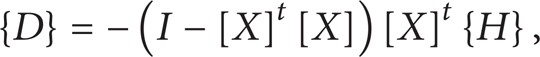
In order to obtain a numerical solution for (32) and (33), the Forsythe method [32] was employed. Curve fitting can be accomplished once {C} and {D} have been successfully estimated by using the least-squares error (LSE) method. Nevertheless, the polynomial coefficients {A} and {B} are the actual expected results for the modal parameter identification; therefore, {A} and {B} should be recovered from {C} and {D}. After utilizing the formulas illustrated in [31, 32], {A} and {B} can be obtained. For the sake of the FRF, measurements can also be represented by a partial fraction form, shown in (6) (for single mode) or the following equation (for multimodes):

$H\left(\omega \right)={\displaystyle \sum }_{k=\mathrm{1}}^{\text{modes}}\left(\frac{R_k}{j\omega -{\sigma }_k-{j\omega }_k}+\frac{R_k^{*}}{j\omega -{\sigma }_k+{j\omega }_k}\right),$

(34)

where R _k is the residue matrix, ω _k is the damped natural frequency, σ _k is the damping coefficient, and * denotes the complex conjugate.

Finally, the mode shape can be identified using (9). The extracted first four mode shapes are given in Figures 5(a)–5(d), shown as a red circle-dash line. It should be noted that one of the superior advantages of the RFP technique, other than the curve fitter, results from the modal parameters, which can be identified even though the measurements are mixed with additive white noise. Regarding the denoising ability of the RFP technique, the measured FRF and calculated FRF by the RFP method at point (6, 4) along the beam are shown in Figure 4. Our comparison results show that the RFP-based curve fitting method can greatly decrease the noise interference.

Figure 4:

Comparison of the measured and the estimated FRF using the RFP method.

Figure 5:

Comparison of the first four mode shapes of an intact beam using the QPP method (blue circle-dash line), RFP method (red circle-dash line), and numerical simulation by ABAQUS (black solid line): (a) Mode Shape 1, (b) Mode Shape 2, (c) Mode Shape 3, and (d) Mode Shape 4.

4.3. Comparison and Discussion

To verify the extracted mode shapes from the aforementioned experiment, we used the commercial FEM software ABAQUS to conduct the numerical computation. The numerical model of the beam for Scenario 1 was established by using a finite element model with 3D “brick” elements in the ABAQUS software. The properties were fed to the beam model, and a free-free boundary condition was used. The Lanczos solver was used to analyze the numerical model. There were three direction results for each mode in ABAQUS; however, only the z direction is of significance. We selected the first 30 eigenvalues as the upper limit of our analysis to guarantee the expected results.

Since the numerical results of mode shapes calculated by ABAQUS are automatically normalized for unity, we normalized the experimental mode shapes vector with respect to its maximum amplitudes. A comparison between the numerical and experimental points of the first four mode shapes is given in Figures 5(a) to 5(d), where the blue circle-dash line represents the experimental mode shape calculated by the QPP method, the red circle-dash line represents the experimental mode shape calculated using the RFP method, and the black line represents the numerical results of the mode shape simulated by ABAQUS software.

The comparison results show that the experimental mode shapes extracted using the RFP method were in agreement with the numerical results, proving to be accurate, whereas the mode shapes calculated by the QPP method were not scaled well, showing some deviation and unsmooth curves compared to the numerical results, especially for the fourth mode shape. The reason for the failure of the QPP method can probably be attributed to the fact that there is a large fluctuation of the FRF imaginary peak values during conditions of uncontrollable impact forces and experimental noise, as in the real-world test. Superior to the QPP, the RFP method makes use of the least-squares error (LSE) to estimate the coefficients of the FRF polynomial. The process of LSE greatly reduces the noise, allowing for the modal parameters (natural frequency, mode shape, and damping) to be obtained by classical theory (as shown in (34)), thus identifying the modal parameters accurately, despite the noise. Moreover, in terms of the applicable conditions, the QPP method is limited to the well-separated modes and lightly damped structure [29]. Conversely, the RFP method can differentiate between closed modes by adding extra terms to the numerator polynomial in order to compensate for the effects of out-of-band modes [31]. To compare the damage detection results using QPP-CWT and RFP-CWT, the rest of the two damaged beams' mode shapes for Scenario 2 and Scenario 3 were also estimated using the two modal parameter identification methods (QPP and RFP).

5. Crack Detection Using CWT Technique

5.1. Edge Effect Phenomenon

For an analysis of the CWT, more data equates to obtainment of better characteristic coefficients. Therefore, a cubic spline interpolation technique was employed to increase the block of the experimental mode shapes. The spline interpolation was applied to each set of 34 measured data points and with a 1 mm interpolation step. Finally, 331 points were derived from the original data. According to the definition described by (12), the CWT is an integration of an analyzed signal and wavelet within an infinite interval. When it is applied to a mode shape with a finite length, distortion phenomenon will appear at the beginning and end of the CWT scalogram, thereby resulting in a misunderstanding when cracks do not exist in the beginning or end of the tested sample. This singular behavior is called the edge effect, and it is the key drawback of the CWT technique when it is applied to space-based damage detection. To solve this problem, Rucka and Wilde extended the original signal by four neighboring points using the cubic spline extrapolation method [16]. In this paper, to avoid any distortion at the boundaries, an extension of the original mode shape was made (Figure 6). The original mode shape was extended by the symmetric mode shape at the two ends about the vertical axis on the horizontal coordinate plane, and then the two symmetric signals were rotated towards the vertical directions. The smooth connection between the original signal and the added signal can remove the distortion caused by the CWT, and the final result shows only those related to the original mode shape.

Figure 6:

Extension of the normalized second mode shape of a tested undamaged beam in Scenario 1.

5.2. Experiment Results and Discussion

The first two mode shapes of the beams obtained for Scenarios 2 and 3 were initially extended and used for CWT analysis. Figure 7 shows the absolute CWT coefficients of the first two extended mode shapes for Scenario 2. In order to compare the two methods, the CWT coefficients were normalized to unity with respect to their maximum absolute values. As seen in Figures 7(a1) and 7(b1), the place where the absolute CWT coefficients' value increased with scale can be explained as an indication of damage at that position [15, 33]. Even though the two methods can identify the crack position using the first mode, there are more irregularities that exist (Figure 7(a1)) when using the QPP-CWT method, which can be attributed to the fact that there exists some external interference, such as noises resulting from a poorly scaled mode shape. This is classified as disturbance. Compared to QPP-CWT, the proposed RFP-CWT method shows clearer results (Figure 7(b1)). Due to the damage located at the node point along the beam, the second mode was not sensitive to the crack and neither of the two methods was able to detect the damage. The higher values of the CWT coefficients for the second mode were produced by the intrinsic mode shape that was not damaged.

Figure 7:

Absolute CWT coefficients of normalized extended mode shapes for Scenario 2 by using the QPP-based method (a1, a2) and the RFP-based method (b1, b2): (a1, b1) for Mode Shape 1 and (a2, b2) for Mode Shape 2.

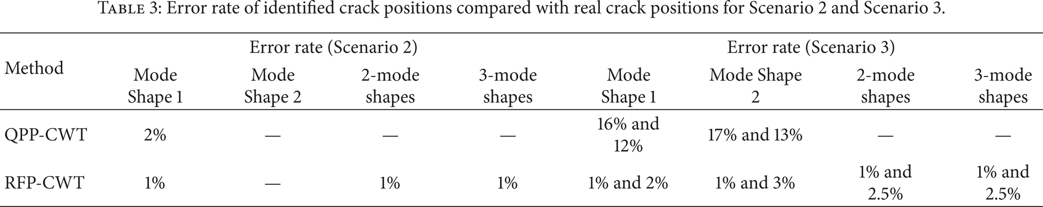
In order to verify the effectiveness of the two methods for multicrack cases, we used Scenario 3. Two cracks were located at 0.25 L and 0.35 L along the beam from the left-hand side. Figure 8 shows the results of the CWT analysis using the first two extended mode shapes for Scenario 3. As previously mentioned, the colored ribbons consisting of the maximum values of the CWT coefficients for each scale are an indication of the effect of the damage. As seen in Figure 8(a1), the first two colored stripes, with higher energy, were considered to be the damaged positions. However, compared with the actual damaged positions, the first colored stripe failed to locate the initial damage due to the experimental noise. The real damage indication was masked by the noise effect located at 0.18 L. Consequently, this method identified the damaged locations as occurring at 0.18 L and 0.23 L. The error rate compared with the real damaged positions was 7% and 12%, respectively (Table 3). A similar occurrence happened to the second mode when using the QPP-CWT method. However, as seen in Figures 8(b1) and 8(b2), more accurate identification resulted when using the proposed RFP-CWT method. Even though there was a smaller noise effect, the damage effect was evident and easily recognizable.

Figure 8:

Absolute CWT coefficients of normalized extended mode shapes for Scenario 3 by using the QPP-based method (a1, a2) and the RFP-based method (b1, b2): (a1, b1) for Mode shape 1 and (a2, b2) for Mode Shape 2.

Comparison of the results from the aforementioned two methods demonstrated that the proposed RFP-CWT method is more accurate and reliable than the conventionally used QPP-CWT method [18] in terms of damage detection. In order to give an overall evaluation of damage detection, we used the summation of the difference in the mode shapes between the damaged beam and the intact beam for our CWT analysis. The equation is

${\text{CWT}}_{\text{comb}}\left(a,u\right)=\text{CWT}\left[{\displaystyle \sum }_{i=\mathrm{1}}^N\left({\phi }_{d,\text{ext}}^i-{\phi }_{u,\text{ext}}^i\right)\right].$

(35)

The normalized CWT expression is given as

${\text{CWT}}_{\text{comb},\text{nor}}\left(a,u\right)=\frac{{\text{CWT}}_{\text{comb}}(a,u)}{\max \left[{\text{CWT}}_{\text{comb}}\left(a,u\right)\right]}.$

(36)

The advantage of the combined mode shape wavelet transform analysis illustrated in (35) is that it not only can solve the problem of a crack that exists at a certain node point, but also causes an accumulation for the damage effect and reduces the inference from the modes that are not sensitive to the damage (e.g., node point mode shape), using a subtracting operation for the mode shapes of the damaged and intact beams (Figure 9). The locations of the damaged positions were accurately identified with little noise effect, particularly for the case of Scenario 3. To investigate further, the first three mode shapes were combined and used for a wavelet analysis. The results of the CWT analysis (Figure 10) showed almost identical results, as the sum of the first two modes was adequate to locate the damaged position for the beam analyzed in this research. In addition, the identified positions and error rates for Scenarios 2 and 3 using the aforementioned crack identification methods are shown in Tables 2 and 3, respectively.

Table 2:

Identified crack position using the methods of QPP-CWT and RFP-CWT for Scenario 2 and Scenario 3.

Method	Scenario 2					Scenario 3
	Mode Shape 1	Mode Shape 2	2-mode shapes	3-mode shapes	Real position	Mode Shape 1	Mode Shape 2	2-mode shapes	3-mode shapes	Real position
QPP-CW	163.2	—	—	—	170	30.6 and 78.2	27.2 and 74.8	—	—	85 and 119
RFP-CW	166.6	—	166.6	166.6	170	81.6 and 125.8	81.6and 129.2	81.6 and 127.5	81.6 and 127.5	85 and 119

Unit: mm.

Table 3:

Error rate of identified crack positions compared with real crack positions for Scenario 2 and Scenario 3.

Method	Error rate (Scenario 2)				Error rate (Scenario 3)
	Mode Shape 1	Mode Shape 2	2-mode shapes	3-mode shapes	Mode Shape 1	Mode Shape 2	2-mode shapes	3-mode shapes
QPP-CWT	2%	—	—	—	16% and 12%	17% and 13%	—	—
RFP-CWT	1%	—	1%	1%	1% and 2%	1% and 3%	1% and 2.5%	1% and 2.5%

Figure 9:

Absolute CWT coefficients of the first two combined mode shape differences: (a) Scenario 2 and (b) Scenario 3.

Figure 10:

Absolute CWT coefficients of the first three combined mode shape differences: (a) Scenario 2 and (b) Scenario 3.

6. Conclusion

This paper presents a novel combination of damage detection methodology, the so-called RFP-CWT approach, for beam-like structures. The first four mode shapes of an intact beam were extracted using the quadrature peaks picking (QPP) method and the rational fraction polynomial (RFP) method in the frequency domain. Validation and comparison were then performed using numerical computations. Our comparison results show that the RFP method was able to more accurately identify the mode shape than the QPP method, especially in light of the unstable input force and experimental noise interference. Furthermore, the damage detection method of QPP-based QPP-CWT and the proposed RFP-based RFP-CWT algorithm using CWT techniques were implemented to identify the damaged positions based on two different scenarios involving damaged beams. Our experimental comparison results suggest that the RFP-CWT method is effective and can accurately locate the damaged position, even for multicracks, whereas the conventionally used QPP-CWT was not able to determine the locations of damage. Finally, an overall evaluation using the sum of the mode shape differences, based on the proposed method, was applied to the damaged structure and was proven to be able to clearly locate the damaged positions.

Conflict of Interests

The authors declare that there is no conflict of interests regarding the publication of this paper.