Sage Journals: Discover world-class research

Abstract

Direct numerical simulations of turbulent viscoelastic fluid flows in a channel with wall-mounted plates were performed to investigate the influence of viscoelasticity on turbulent structures and the mean flow around the plate. The constitutive equation follows the Giesekus model, valid for polymer or surfactant solutions, which are generally capable of reducing the turbulent frictional drag in a smooth channel. We found that turbulent eddies just behind the plates in viscoelastic fluid decreased in number and in magnitude, but their size increased. Three pairs of organized longitudinal vortices were observed downstream of the plates in both Newtonian and viscoelastic fluids: two vortex pairs were behind the plates and the other one with the longest length was in a plate-free area. In the viscoelastic fluid, the latter vortex pair in the plate-free area was maintained and reached the downstream rib, but its swirling strength was weakened and the local skin-friction drag near the vortex was much weaker than those in the Newtonian flow. The mean flow and small spanwise eddies were influenced by the additional fluid force due to the viscoelasticity and, moreover, the spanwise component of the fluid elastic force may also play a role in the suppression of fluid vortical motions behind the plates.

1. Introduction

It is common knowledge that a surfactant or polymer additive can suppress turbulence and significantly reduce turbulent frictional drag when added to a liquid in a turbulent pipe flow [1, 2]. In general, the solution used as a working fluid for such a drag-reducing fluid exhibits viscoelasticity giving rise to significant modulations of fluid motions in turbulent flows as well as in laminar ones. From the practical viewpoint, the understanding of the turbulence characteristics in viscoelastic fluids is important, since it is believed that this can help in improving performance and fluid controls in relevant engineering situations. For instance, the drag-reducing surfactant solution liquid has been applied as an energy-saving transport medium in residential heating devices and is currently being tested for further practical applications [3]. In flows accompanied by temperature and concentration gradients, the convective heat or mass transfer also appears to be decreased due to the damped momentum exchange. In other words, the suppression of turbulence reduces pumping energy and also pipe heat loss. The reduction of wall heat transfer is not always an advantage if one considers that more effort is needed in heat exchanger performance. Therefore, it is of practical value to develop an effective method to locally enhance the heat transfer. Our interest in this work focuses on viscoelastic fluid flows past a bluff body that may trigger a flow separation and reattachment and that generates longitudinal (streamwise-oriented) vortex pairs, which may locally enhance the heat and momentum transfer.

In the following, let us briefly review the numerical and experimental works relating to the present research. Fundamental studies by means of direct numerical simulation (DNS) have been increasingly performed to investigate modulated flow structures and the mechanism of drag reduction in viscoelastic turbulent flows. In those studies, most of the earlier DNS with several viscoelastic fluid models was limited, especially in the smooth pipe, plane channel, and boundary layer. Sureshkumar et al. [4] adopted the finitely extensible, nonlinear elastic-Peterlin (FENE-P) model and demonstrated the first DNS on viscoelastic turbulent channel flow. Min et al. [5] employed a different constitutive equation model, the Oldroyd-B model, and Yu et al. [6, 7] used the Giesekus model and compared their results with experiments on surfactant solutions. Tamano et al. [8, 9] performed DNS on the zero-pressure-gradient drag-reduced turbulent boundary layer in viscoelastic fluids using all of these models. With the aid of these DNS approaches, substantial new knowledge on the relation between the drag reduction and rheological properties of viscoelastic solutions, for example, the relaxation time and the elongational viscosity, has been gained during this decade. In terms of the relation between the turbulence structures and the additional stress due to the additive, many researchers have demonstrated the interactions between the near-wall coherent structures and the fluid viscoelasticity [10 –13]. In particular, Kim et al. [12, 13] reported a dependency of the vortex-strength threshold for the autogeneration of new hairpin vortices in the buffer layer on viscoelasticity. In their simulations of drag-reducing channel flows, a moderate Weissenberg number of Wi_τ = 50, defined as the ratio of the polymer relaxation time to the wall time scale, was found to inhibit the generation of new vortices by polymer-induced countertorques, generating fewer vortices in the buffer layer. This implies that the viscoelastic-force torque would retard the vortical motion and the Reynolds-stress production. By the way, longitudinal (streamwise-oriented) vortices have enormous utility for flow control and are capable of producing beneficial effects in transport enhancement. They are utilized because they have great practical importance. Experimental investigations by Fiebig et al. [14] revealed the enhancement of heat transfer in the presence of longitudinal vortices, which were triggered by vortex generators (VG). Liou et al. [15] measured detailed local Nusselt number distributions with twelve different-shaped longitudinal VG. As for the viscoelastic fluid, Eschenbacher et al. [16, 17] experimentally investigated the effect of longitudinal vortices on the wall heat transfer using a single wing-type VG in drag-reducing surfactant solution flows. They observed that the longitudinal vortex behind the VG played an important role in heat transfer enhancements and might recover the reduced wall heat transfer coefficient of the surfactant solution up to the maximum value of pure water. Similar conclusions were drawn by other researchers in different experiments [18, 19]. Moreover, it was shown that the longitudinal vortex remained far downstream of the VG due the dumped momentum exchange in a drag-reduced flow and thereby enhanced the heat transfer in the wake of the VG [16]. This experimental fact may be in contradiction to the numerically observed viscoelastic behavior, namely, the countertorque against vortical motions mentioned above. In our previous works [20 –23], we investigated the viscoelastic turbulent flow behind a two-dimensional rectangular rib and demonstrated that the quasistreamwise turbulent eddies survived far downstream, while the spanwise eddies were suppressed. However, we have currently not elucidated the counteracting characteristics of the viscoelastic force against the large-scale longitudinal vortices generated in the (time-averaged) mean flow behind a finite plate.

As already mentioned, it is known that, on a smooth wall, the intensity of the near-wall turbulent eddies is reduced and their sizes are increased mostly in the buffer layer. This provides evidence for the drag-reduction mechanism based on modulations of near-wall eddies, which facilitate significant amounts of turbulence production. On the other hand, with a bluff body like a rib, the eddies are decreased in number, but quasistreamwise vortices remain. In that sense, the behavior and effect of the longitudinal vortex behind a plate in a viscoelastic flow are still unclear, since there are very few DNSs of viscoelastic turbulent flows in complex geometries. In the present study, we performed a DNS of viscoelastic-fluid flows in a channel with wall-mounted plates in order to analyze the turbulence and the effect of an obstacle that triggers longitudinal vortices.

2. Computational Approach

The computational domain we employed here is shown in Figure 1. Periodically repeating spatial units of three-dimensional solid plates are simulated with the periodic boundary conditions in the streamwise (x) and spanwise (z) directions. While the computational domain is 12.8δ × 2δ × 6.4δ, the dimensions of the plate are 0.1δ × 0.5δ × 3.2δ in x, y, and z, respectively. Two plates are installed at the coordinate origin (x, z) = (0, 0) on each wall surface, but the front face of each plate is set at x = 0. The nonslip and nonpenetrative boundary condition is applied to the whole solid wall, including the plate surface. The nondimensional governing equations are the equation of incompressible continuity

\nabla \cdot u = 0,

(1)

the Navier-Stokes equation

\partial_{t^{*}} u^{+} + (u^{+} \cdot \nabla) u^{+} = - \nabla p^{+} + f + e + f_{i m},

(2)

where

f = \frac{β}{R e_{τ 0}} \frac{\partial^{2} u_{i}^{+}}{\partial {x_{j}^{*}}^{2}},

(3)

e = \frac{1 - β}{W i_{τ 0}} \frac{\partial c_{i j}}{\partial x_{j}^{*}},

(4)

and the constitutive equation based on the Giesekus model

\frac{\partial c_{i j}}{\partial t^{*}} + u_{k}^{+} \frac{\partial c_{i j}}{\partial x_{k}^{*}} - \frac{\partial u_{i}^{+}}{\partial x_{k}^{*}} c_{k j} - c_{i k} \frac{\partial u_{j}^{+}}{\partial x_{k}^{*}} + \frac{R e_{τ 0}}{W i_{τ 0}} [c_{i j} - δ_{i j} + α (c_{i k} - δ_{i k}) (c_{k j} - δ_{k j})] + κ \frac{\partial^{2} c_{i k}}{\partial x_{k}^{* 2}} = 0 .

(5)

In the above equations, u = u_i = (u₁,u₂,u₃)≡(u, v, w), p, t, and c_ij denote the velocity vector, the pressure, the time, and the conformation tensor. The quantities with superscript (⁺) indicate that they are normalized by the friction velocity u_τ0, which is derived from the mean pressure gradient through the computational volume, in the case of a smooth channel without any obstruction:

u_{τ 0} = \sqrt{- \frac{δ}{ρ} \cdot \frac{Δ p}{L_{x}}} .

(6)

Here, ρ is the fluid density. As for t* and x*, they are normalized by δ/u_τ0 and δ, respectively. In (2), β = η_s/η₀ means a ratio of the solvent viscosity η_s to the total zero-shear-rate solution viscosity η₀, and the last term of f_i in the right-hand side represents the body force vector per unit volume for the immersed boundary method [24]. The nondimensional value α in (5) is the mobility factor, which determines the extensional viscosity of a fluid. The friction Reynolds number, the bulk mean Reynolds number, and the Weissenberg number are defined, respectively, as Re_τ0 = ρu_τ0δ/η₀, Re_m = 2ρU_mδ/η₀ (U_m, the bulk mean velocity, as defined later), and Wi_τ0 = ρλu_τ0²/η₀ (λ, the relaxation time). The specific control-parameter values we tested here are summarized in Table 1. In the present study, we compared the flow fields at different Weissenberg numbers (including the Newtonian fluid with Wi_τ0 = 0), while the friction Reynolds number corresponding to the pressure difference between the inlet and outlet of the domain of interest was fixed at a constant.

Table 1:

Fluid and mean-flow parameters.

Fluid	Wi_τ0	α	β	Re _τ0	Re _m	U _m ⁺

Newtonian	—	—	1.0	100	1224	6.12
Viscoelastic	12	0.001	0.9	100	1276	6.38
Viscoelastic	20	0.001	0.9	100	1288	6.44

Figure 1:

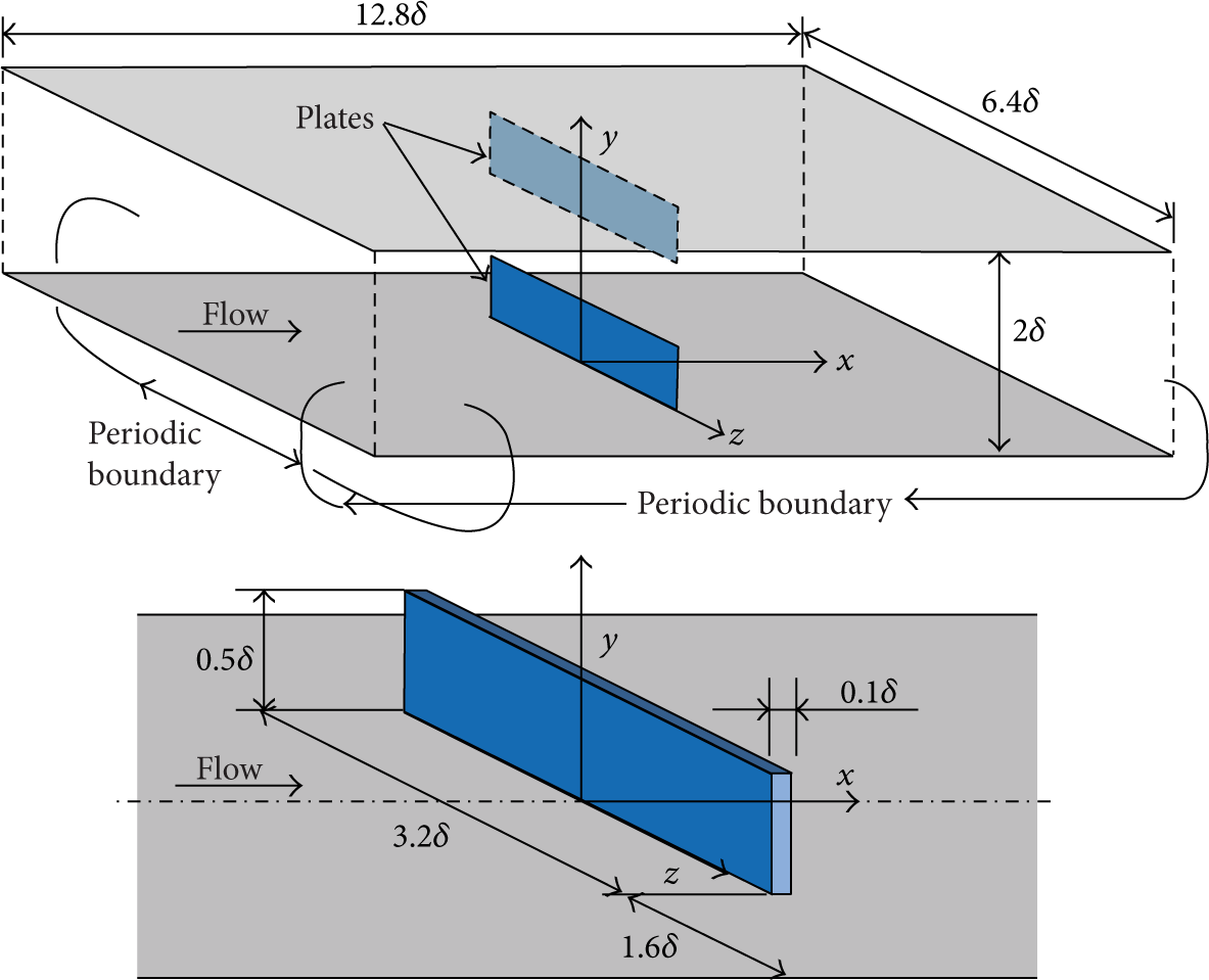
Configuration of flow channel and detail of a wall-mounted finite plate.

For spatial discretization, the finite different method was used. A central scheme with fourth-order accuracy was applied in the x and z directions and the second-order accuracy was in the y direction. Time advancement was done using the third-order Runge-Kutta method, but the second-order Crank-Nicolson method was used for the viscous terms in the y direction. For numerical stability, we employed a flux-limiter scheme (MINMOD) to discretize the convective term in (5) and also introduced an artificial diffusion term as described in the last term in the left-hand side of the equation, where κ* means a numerical diffusivity. The present calculations were stable under the condition of κ* = 2 × 10⁻⁴. Figure 2 shows the shape of the grids we applied. The minimum grid spacing Δy_min⁡⁺ = 0.31 to resolve steep velocity gradients is ensured near the plate edge and the channel wall, while the uniform meshes were used in the horizontal directions with Δx⁺ = 10 and Δz⁺ = 5. The complete grid size was 128 × 96 × 128.

Figure 2:

Computational grids with emphasis on the plate, viewed from the spanwise direction.

3. Results and Discussion

3.1. Suppression of Turbulence

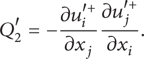
Figure 3 presents an instantaneous snapshot of eddies and streamwise velocity fluctuations near the bottom wall in each of the Newtonian and viscoelastic flows. Note that all the flows presented in this paper were obtained under the same pressure loss of Re_τ0 = 100, but the bulk Reynolds number varied between 1224 and 1288, as given in Table 1. Thick black lines in the x-z contour represent the isoline of u = 0, and thus the inside blue area corresponds to a reverse flow. Here, eddies are visualized by the second invariant of the fluctuating velocity-gradient tensor:

Q_{2}^{'} = - \frac{\partial u_{i}^{' +}}{\partial x_{j}} \frac{\partial u_{j}^{' +}}{\partial x_{i}} .

(7)

As shown in Figure 3(a), we categorize two regions where the flow was either directly or not directly obstructed by the upstream/downstream plate as the “upstream/downstream plate” or “plate-free region.” Hereafter, they are called “area A” and “area B,” respectively. The demarcations between them are located at z* = z/δ = ±1.6, as indicated by broken lines in the visualization figures.

Figure 3:

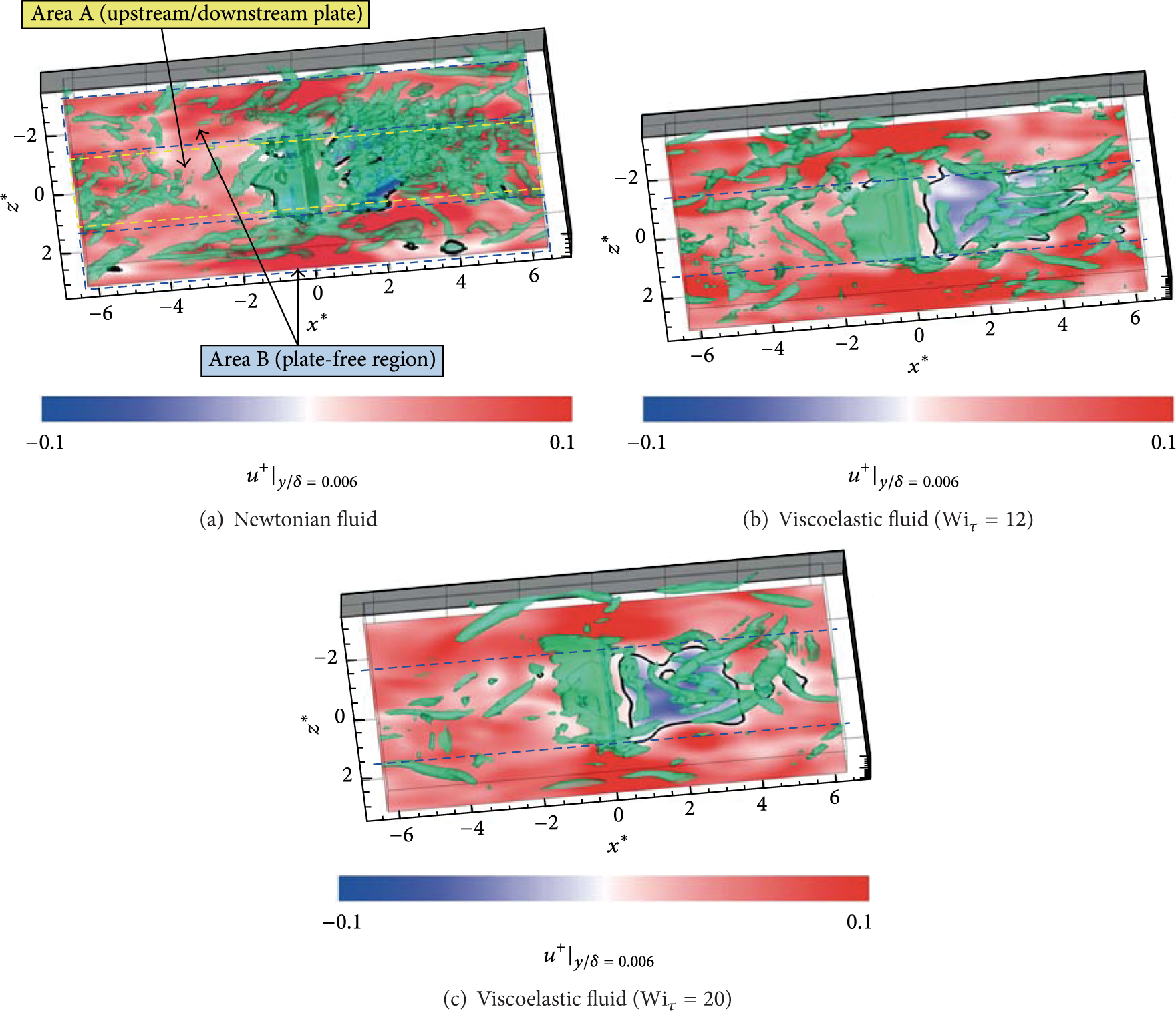
Streamwise velocity in the vicinity of the wall (contour) and visualization of instantaneous vortex structures (isosurface) in the bottom half of the channel: isosurfaces of the second invariant of the deformation tensor, Q₂′ = − 0.01. The main flow moves from left to right. Two areas labelled as either “A” or “B” are defined explicitly in (a), and only their demarcations are presented in (b) and (c).

In Figure 3(a), a number of small-scale eddies can be observed to occur just behind the plate (in area A) and they propagate far downstream. Then, they seem to approach the next downstream plate due to the periodicity of the computational domain, but most of them decay or break rapidly before reaching the plate. This is because the bulk Reynolds number is too low to produce and sustain turbulence in a smooth channel compared to high viscous dissipation. In addition, strongly curved streamlines and local acceleration of the flow in front of the plate may also be attributed to the rapid decay of eddies. From Figures 3(b) and 3(c), it is found that the eddies in the viscoelastic fluids are generally larger in size but smaller in number than those observed in the Newtonian fluid. The quasistreamwise eddies are further elongated along the streamwise (x) direction in the viscoelastic fluid, especially for Wi_τ0 = 20. In the area far downstream (or upstream) of the plate, there remain only eddies that are relatively large and elongated in the streamwise direction. Spanwise eddies are observed locally just behind the plate and then they disappear a short distance from it, while many longitudinal eddies dominantly occur near the reattachment point. This character of the turbulent eddies behind a bluff body is consistent with that observed in the orifice flow [20, 22], which demonstrates that the spanwise eddies induced by the Kelvin-Helmholtz instability would be suppressed significantly in viscoelastic flows at high Weissenberg numbers. In area B, relatively larger eddies compared to those in area A are observed, especially in the Newtonian fluid. The number of eddies is smaller but the scale of the eddies increases and longitudinal eddies appear dominantly, mostly originating from plate-induced eddies in area A. Housiadas and Beris [25] showed the energy spectra of a viscoelastic turbulent flow through a smooth channel and reported that, in the viscoelastic flow, low wave number contributions increase in intensity, whereas those with a high wave number decrease in proportion to the Weissenberg number. The same phenomenon is probably occurring in the present case. Relatively small eddies seen in the Newtonian flow are suppressed in the viscoelastic flows and large-scale eddies with highly turbulent energy survive. In the viscoelastic flow at Wi_τ0 = 20, the number of vortices is decreased compared with the case for Wi_τ0 = 12, especially, in the plate upstream of area A and the whole region of area B.

In order to extract the Kelvin-Helmholtz (K-H) eddies and examine the associated fluid forces on the eddies, the flow and force fields just behind the plate are visualized in Figures 4 and 5. Here, the downstream of the plate mounted on the bottom channel wall and at z = 0 is in focus. Figure 4 shows contours of the swirling strength λ_ci,z, by which underlying spanwise eddies can be extracted by excluding the contributions of shearing motions [26]. We computed λ_ci,i at each grid point as an imaginary part of the complex eigenvalues of the two-dimensional velocity-gradient tensor ∂u_j/∂x_k (here, both j and k are perpendicular to the i direction): a vortical motion is easily identified by plotting isoregions of λ_ci,i > 0. Rotation direction is defined with the sign of local vorticity ω_z. The plate is located at x* = 0.0–0.1. In the region shown in Figure 4, there is a high-speed core area of the contraction flow past the two plates and also a low-speed area corresponding to the recirculation zone behind the plate. The velocity gradient between these areas (at around y* = 0.5) is large, so the K-H vortices (characterized by blue contour in Figure 4) are sequentially induced. In Figure 4(a), the large λ_ci,z represents the existence of K-H vortices in the Newtonian fluid. The scale of each eddy is smaller than 0.5δ but many strong eddies are visible in x = 1–3. On the other hand, in the viscoelastic fluid, relatively large-scale but few eddies appear and they are weaker than those in the Newtonian fluid.

Figure 4:

Contour of swirling strength λ_ci,zω_z/|ω_z| in the separated shear layer just behind the plate edge in the plane of z = 0: positive, counterclockwise rotation and negative, clockwise rotation. The main flow direction is from left to right.

Figure 5:

Velocity vectors of a spanwise vortex in the separated shear layer, which is highlighted with a red frame in Figure 4(b), and the viscous and elastic forces acting on the vortex. The contour in (a) shows the swirling strength and that in (b) and (c) represents the inner product of the velocity vector and the vector of either the viscous force or the elastic force.

Figure 5(a) shows one of the K-H eddies in the viscoelastic flow. In Figures 5(b) and 5(c), vector fields corresponding to the viscous and elastic forces acting on the eddy or the surrounding flow motion are presented, and each contour shows the alignment degree between the flow vector and individual force in order to examine the relationship between the vortical motion and associated individual force. Specifically, the vector alignment is quantified by an inner product of two vectors:

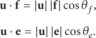
\begin{matrix} u \cdot f = | u | | f | \cos θ_{f}, \\ u \cdot e = | u | | e | \cos θ_{e} . \end{matrix}

(8)

The vectors f and e are the viscous and elastic forces calculated with (3) and (4), respectively; θ_f and θ_e represents the angle between the local velocity vector and either the viscous or elastic force. From Figure 5(b), we can confirm that the viscous force works in the opposite direction to the vortical motion. It should be noted that the local minimum position of λ_ci,zω_z/|ω_z| is marked in Figure 5, in addition to the rotation center in terms of the instantaneous streamlines. As for the elastic force given in Figure 5(c), the inner product appears positive near the vortex center, but this is the case only for the upper side of the vortex. In the lower side, the inner product appears to be negative. The same tendency has also been confirmed in Wi_τ0 = 20, although not shown in the figure. Therefore, it can be concluded that the spanwise primary K-H eddies would be damped by both the viscosity and elasticity, which would result in the suppression of turbulence behind the plate in area A.

3.2. Influence on Time-Averaged Vortex Structures

Figure 6 shows the organized vortex structures in the mean flow and the contour of the skin-friction coefficient calculated with time-averaged data. The vortices are visualized by the second invariant of the time-averaged velocity-gradient tensor:

\bar{Q_{2}} = - \frac{\partial U_{i}^{+}}{\partial x_{j}} \frac{\partial U_{j}^{+}}{\partial x_{i}} .

(9)

Note that $\bar{Q_{2}}$ is based on the time-averaged velocity, U_i(x,y,z) = ∫‍u(x,y,z,t)dt/ΔT. The time-averaged skin-friction coefficient C_f is determined by

C_{f} (x, z) = \frac{τ_{w} (x, z)}{1 / 2 ρ U_{m}^{2} S} = \frac{2}{U_{m}^{+ 2}} {[\frac{β}{R e_{τ 0}} \frac{\partial U^{+}}{\partial y^{*}} + \frac{1 - β}{W i_{τ 0}} C_{12}]}_{y = 0},

(10)

where τ_w(x,z) is the local wall shear stress and U_m is the bulk mean velocity given by

U_{m} = \frac{\int_{0}^{L_{z}} ‍ \int_{0}^{2 δ} ‍ U (x, y, z) d y d z}{\int_{0}^{L_{z}} ‍ \int_{0}^{2 δ} ‍ d y d z}

(11)

at arbitrary x (since U_m does not depend on x according to the mass conservation law).

Figure 6:

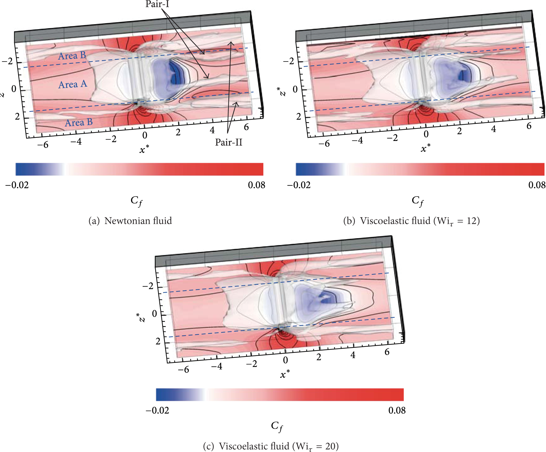
Contour of time-averaged local skin-friction coefficient and time-averaged vortex structures in the bottom-half channel: isosurfaces of the second invariant of the deformation tensor, $\bar{Q_{2}} = - 5.0 \times 10^{- 5}$ . The main flow moves from left to right. The blue broken lines represent the demarcations of areas A and B.

The highest frictional drag clearly appears near the spanwise plate edges (in area B) because of a contracted high-speed flow between spanwise neighboring plates (Figure 6). Behind the plate, it is clearly observed that four tails (corresponding to four vortices) extend from the plate edges to far downstream; that is, large-scale longitudinal vortices appear as secondary flows. According to reflection symmetry with respect to z = 0, two pairs of longitudinal vortices may be detected from the Figure. One of the pairs originates from a horseshoe vortex occurring in front of the plate and located slightly outside area A: this vortex pair is labelled as “pair-I vortex”; see Figure 6(a). The other vortex pair, to be called the “pair-II vortex,” appears in area A and emerges near the top corners of the plate. These two pairs are observed in all of the flows, but the vortices, especially pair-II, become obviously weaker and shorter as the Weissenberg number increases. In any case, relatively large frictional drag occurs on the wall surface near the vortices.

The direction of vortical motion is not taken into account in the vortex visualization using $\bar{Q_{2}}$ as in Figure 6. The vortices can be divided into components by means of mean-flow swirling strength (Λ_ci,i based on ∂U_j/∂x_k), which allows us to extract only longitudinal (streamwise-oriented) vortices, as given in Figure 7(a). In this Figure, there are six longitudinal vortices or three vortex pairs. The wall-normal vortices are also shown in Figure 7(b) and they occur in the form of twin vortices due to separation just behind the plate, which is reported in many studies dealing with fluid flow around rectangular obstacles [27, 28]. The pair-II vortices may have their roots in this wall-normal vortex pair. As for the streamwise vortices in Figure 7(a), another pair of small longitudinal vortices (named the “pair-III vortex”) that could not be visualized in Figure 6 is found near the central plane at z = 0. Since the vortices seem not to be derived from the plate and occur around the mean-flow reattachment zone, they may be induced by the pair-II vortices. The pair-III vortices shift downstream as the Weissenberg number increases (figure not shown): the region where the swirling strength is over 2 appears in x* = 1.2–4.9 in the Newtonian fluid, x* = 1.6–5.4 for Wi_τ0 = 12, and x* = 2.2–5.9 for Wi_τ0 = 20. This downstream shift accords well with that observed in the mean-flow reattachment region, which moves further from the plate with increasing Weissenberg number; see also Figure 6. Hence, the pair-III vortex may be closely related to the flow reattachment. If so, the vortex would induce enhancement of heat transfer in this area.

Figure 7:

Isosurfaces of streamwise and wall-normal components of swirling strength in the Newtonian fluid flow with emphasis on the area downstream of the plate. The main flow moves from top left to bottom right. The broken square indicates the plate location. The mean-flow swirling strength Λ_ci,i is defined as an imaginary part of the complex eigenvalues of the mean velocity-gradient tensor ∂U_j/∂x_k.

Figure 8 shows the mean streamlines in the cross-section at x* = 5.0 with a background contour of λ_ci,x showing the strength of the longitudinal vortices. A comparison between the Newtonian flow and the viscoelastic flow at Wi_τ0 = 20 implies the robustness of the longitudinal vortices but reveals a large variation in the streamlines, especially, behind the plate. The pair-I vortices are weaker in the viscoelastic flow. The strength of the pair-II vortices is almost unchanged, while their shape is unclear in the viscoelastic flow from the viewpoint of cross-section streamlines. The pair-III vortices located at z* = ±0.2 seem to be enhanced in the viscoelastic flow, because their appearance is moved slightly downstream, as mentioned above. The large variation of the streamlines behind the plate may be due to elasticity of the fluid. In the following section, we focus on the elastic force in the same cross-section to elucidate its relationships with the vortices and the mean flow.

Figure 8:

Mean-flow streamlines in the y-z plate at x* = 5.0 and contour of streamwise swirling strength Λ_ci,x.

3.3. Forces Acting on Longitudinal Vortices

The fluid forces exerted on the fluid itself are examined in Figure 9, focusing on the organized longitudinal vortices of pairs-I–III at the same streamwise location as Figure 8. According to reflective symmetry with respect to z = 0, only half of the cross-section in the spanwise direction is shown. Figure 9(a) presents the swirling strength distribution of Λ_ci,x, where three vortices are observed: the vector represents the mean velocity (V, W), and Figures 9(b) and 9(c) show, respectively, the mean viscous force ( F ) and the mean elastic force ( E ). The contours show the inner products between the mean-flow vector U and each time-averaged force, in order to examine the relationship between the vortex motion and individual force.

Figure 9:

Time-averaged flow and force fields around the longitudinal vortices at x* = 5.0 for the viscoelastic fluid (Wi_τ0 = 20). The green isolines indicate Λ_ci,x = 2.

In Figure 9(b), it can be seen that the viscous-force direction is almost opposite to the velocity in every location. The inner product between them is negative around the vortices. In other words, the viscous force and the flow direction are always in anticorrelation. Therefore, it can be said that the viscous force suppresses longitudinal vortices. As for the elastic force, its vector field does not reveal rotating behavior near the vortices, unlike the viscous force, as seen in Figure 9(c). The elastic force seems to force fluid to move globally from the bottom left to the top right in the figure, independently of the underlying vortices. However, in the vicinity of the wall, the force is opposite to the velocity direction. The inner product between the velocity and the elastic force around the longitudinal vortices exhibits both positive and negative values. Around the pair-I vortex, the absolute value of the positive inner product is lower than that of the negative. This implies that, regardless of the existence of a localized region where longitudinal vortices are promoted, the elastic force suppressed vortices, especially near the wall.

Figure 10 shows the contours of the wall-normal and spanwise components of the elastic force acting on the longitudinal vortices at x* = 5, where the largest magnitude of the wall-normal elastic force appears around the pair-III vortex for Wi_τo = 20. The green lines in the figure represent the longitudinal vortices, as also presented in Figure 9. As for the pair-I vortex, the spanwise force E_z works strongly in an opposite direction to the rotating direction in the near-wall region accompanied by strong shear. In the upper and lower sides of the pair-II and pair-III vortices, E_z reveals an inverse correlation with the fluid rotating motion. In the vicinity of the wall, a strong spanwise force is observed mainly in area A. On the other hand, in Figure 10(a), the wall-normal force E_y around the pair-I vortex is weaker than around other vortices. The force in area A is greater than that in area B, especially, in the region between pair-III vortices. Figure 11 shows the relationship between the maximum swirling strength relating to the pair-III vortices and the integrating value of E_y at z = 0. The latter value is given as ∫₀¹‍E_ydy*. The behaviors of Λ_ci,x|_max and ∫₀¹‍E_ydy* as a function of x are similar to each other and their local maxima are close to each other. It may be conjectured that there is a relationship between the pair-III vortex and the wall-normal elastic force. In summary, it can be said that the spanwise elastic force would suppress the longitudinal vortices in most areas, while the wall-normal force does not so affect longitudinal vortices except for the pair-III vortices.

Figure 10:

Wall-normal and spanwise elastic forces in the y-z plate at x* = 5.0 for the viscoelastic fluid (Wi_τ = 20). The green isolines indicate Λ_ci,x = 2 as similarly to Figure 9.

Figure 11:

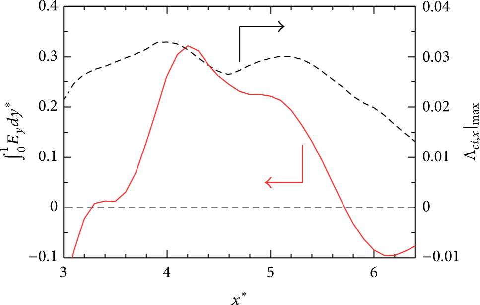
Comparison of integrated wall-normal elastic force at z = 0 and the maximum swirling strength at z* = 0.3 in the viscoelastic fluid flow for Wi_τ0 = 20.

3.4. Local Skin-Friction Drag and Net Drag Reduction

Figure 12 shows the distributions of the local C_f value along the spanwise axis at x* = 5.0 and 8.4 for each flow case. The highest frictional-drag area appears near each spanwise edge of the plate, or at the demarcation between area A and area B, and is also near the reattachment point of the pair-I vortex (see also the streamlines presented in Figure 8). The difference in C_f between the Newtonian and viscoelastic fluids is large in area A between the maximum C_f points, while the pair-I vortices are suppressed strongly in this area. However, at x* = 8.4, the suppression of the pair-I vortex is rather weak and hence the difference in C_f is small compared to that at x* = 5.

Figure 12:

Local skin-friction coefficient along the spanwise direction at different streamwise locations.

Figure 13 presents the drag-reduction percentage DR%, which is defined as

DR % (x, z) = 1 - \frac{{[C_{f} (x, z)]}_{viscoelastic}}{{[C_{f} (x, z)]}_{Newtonian}},

(12)

where Re_m for two corresponding fluids under the same Re_τ0 condition are compared. A negative DR% indicates an increase in the flow resistance for the relevant viscoelastic fluid flow.

Figure 13:

Local drag-reduction rate along the spanwise direction at different streamwise locations.

At x* = 5, the maximum drag reduction occurs around z* = ±0.6 (Figure 13), which is nearer to the center of area A compared to the location of the maximum skin friction that appears at z* ≈ ±1.5 (Figure 12). When focusing on the highest drag-reduced location, one may see that it is near the pair-II vortex, which is weakened strongly in the viscoelastic fluid. However, DR% at the center of area A is not so high and is almost the same level as that in area B at the further downstream region of x* = 8.4, where the pair-II vortex is weakened (or decayed) in both fluid cases. The suppression of turbulence originating from the K-H instability just behind the plate is also the main cause of the high DR% found at x* = 5. Since the turbulent fluctuation decays rapidly and almost settles down at x* = 8.4, the difference in C_f between the Newtonian and viscoelastic flows becomes relatively small in the far downstream region. Although the suppression of the pair-I vortex is significant, the highest drag reduction occurs in the region just beneath the pair-II vortex. In regard to the pair-III vortex, its swirling strength in the viscoelastic flow is greater than that in the Newtonian flow because this vortex is shifted in the streamwise direction. Therefore, the effect of the pair-III vortex on the frictional drag is weak, compared to the other vortex pairs. It seems that the suppression of the pair-II vortex affects frictional drag significantly. The skin-friction drag is lower than that in the Newtonian fluid in the whole area.

Figure 14 shows profiles of the spatially averaged drag-reduction percentage as a function of z as follows:

〈 DR % 〉 = \frac{1}{L_{x}} \int_{0}^{L_{x}} ‍ | DR % | d x .

(13)

The drag-reduction rate is not spatially uniform and is remarkably different between area A and area B. In area A, high drag reductions are obtained: 〈DR%〉 ≈ 30% at Wi_τ0 = 12 and 40% at Wi_τ0 = 20, while area B reveals relatively low drag reduction. The center of area B (z* = ±3.2), the furthest from the plate, exhibits small drag reductions of 〈DR%〉 = 12%–15%. The spanwise location at which the maximum drag reduction appears is found at z* = ±0.9. A reason for this is the influence of the vortex pairs; that is, the suppression of the pair-II vortex and the decrease in drag near the reattachment point might lead to the drag reduction. Other local peaks appear at z* = ±1.8 and they may be due to the suppression of the K-H instability at the spanwise edge of the plate.

Figure 14:

Spanwise distribution of streamwise-averaged drag-reduction rate, defined by (13).

Figure 15 shows distributions of the local skin-friction coefficient C_f defined by (10) at the centers of either area A (z = 0) or area B (z* = 3.2). Also shown is the distribution on the line of z* = 0.8, at which the maximum of 〈DR%〉 appears. At z = 0, a significant reduction occurs to some extent behind the plate, because of the suppression of the K-H and turbulent eddies, similar to the case of the rib-mounted channel flow [21]. At z* = 0.8, the difference in C_f between the two fluid cases is large in the downstream of the recirculation area (x* = 3.6–6.4), where the pair-II vortex is observed in the Newtonian flow. On the other hand, moving downstream of the area, the difference becomes small. This implies that the suppression of the pair-II vortex induces a decrease in the momentum transport in x* = 3.6–6.4. At z* = 3.2, the differences in the frictional drag are less significant and, hence, it can be said that contribution of longitudinal vortices in area B is very weak.

Figure 15:

Time-averaged local skin-friction coefficient at z* = 0 (plate center), 0.8, and 3.2.

4. Conclusion

The effects of fluid viscoelasticity, governed by the Giesekus model, on the evolution of longitudinal vortex behind finite plates in a channel flow were studied by means of direct numerical simulation. The following results are expected to contribute to our understanding of organized longitudinal vortices and of the characteristics of the viscoelastic turbulent flow in a complex geometry.

We observed that three pairs of large-scale vortices occurred behind the plates and they were weakened in the viscoelastic fluid. The suppression of longitudinal vortices was induced by the elastic force as well as the viscous force. The spanwise elastic force works opposite to longitudinal vortices, while the wall-normal component does not play a role in the longitudinal-vortex suppression. The suppressions of the longitudinal vortices and the turbulent fine-scale eddies from the Kelvin-Helmholtz instability caused a significant drag reduction to some extent behind the plates. In case of higher Reynolds numbers, a somewhat larger value for the drag-reduction rate would be obtained because of further suppression of near-wall turbulence.

Conflict of Interests

The authors declare that there is no conflict of interests regarding the publication of this paper.

Footnotes

Acknowledgments

This work was partially supported by Grants-in-Aid for Scientific Research (C) no. 25420131 from Japan Society for the Promotion of Science (JSPS). The present simulations were performed using the super supercomputing resources at Cyberscience Center, Tohoku University, and at Cybermedia Center, Osaka University.

References

Gyr

and Bewersdorff

H. W.

, Drag Reduction of Turbulent Flows by Additives, Kluwer Academic Publisher, Dordrecht, The Netherlands, 1995.

F. C.

Wei

J. J.

, and Kawaguchi

, Turbulent Drag Reduction by Surfactant Additives, John Wiely & Sons, Singapore, 2012.

Takeuchi

, “Demonstration test of energy conservation of central air conditioning system at the Sapporo City Office Building, reduction of pump power by flow drag reduction using surfactant,” Synthesiology, vol. 4, no. 3, pp. 132–139, 2011.

Sureshkumar

Beris

A. N.

, and Handler

R. A.

, “Direct numerical simulation of the turbulent channel flow of a polymer solution,” Physics of Fluids, vol. 9, no. 3, pp. 743–755, 1997.

Min

Yoo

J. Y.

Choi

, and Joseph

D. D.

, “Drag reduction by polymer additives in a turbulent channel flow,” Journal of Fluid Mechanics, no. 486, pp. 213–238, 2003.

and Kawaguchi

, “Direct numerical simulation of viscoelastic drag-reducing flow: a faithful finite difference method,” Journal of Non-Newtonian Fluid Mechanics, vol. 116, no. 2–3, pp. 431–466, 2004.

, and Kawaguchi

, “Numerical and experimental investigation of turbulent characteristics in a drag-reducing flow with surfactant additives,” International Journal of Heat and Fluid Flow, vol. 25, no. 6, pp. 961–974, 2004.

Tamano

Itoh

Hoshizaki

, and Yokota

, “Direct numerical simulation of the drag-reducing turbulent boundary layer of viscoelastic fluid,” Physics of Fluids, vol. 19, no. 7, Article ID 075106, 17 pages, 2007.

Tamano

Graham

M. D.

, and Morinishi

, “Streamwise variation of turbulent dynamics in boundary layer flow of drag-reducing fluid,” Journal of Fluid Mechanics, vol. 686, pp. 352–377, 2011.

10.

Dubief

White

C. M.

Terrapon

V. E.

Shaqfeh

E. S. G.

Moin

, and Lele

S. K.

, “On the coherent drag-reducing and turbulence-enhancing behaviour of polymers in wall flows,” Journal of Fluid Mechanics, vol. 514, pp. 271–280, 2004.

11.

Roy

Morozov

van Saarloos

, and Larson

R. G.

, “Mechanism of polymer drag reduction using a low-dimensional model,” Physical Review Letters, vol. 97, no. 23, Article ID 234501, 4 pages, 2006.

12.

Kim

Adrian

R. J.

Balachandar

, and Sureshkumar

, “Dynamics of hairpin vortices and polymer-induced turbulent drag reduction,” Physical Review Letters, vol. 100, no. 13, Article ID 134504, 4 pages, 2008.

13.

Kim

and Sureshkumar

, “Spatiotemporal evolution of hairpin eddies, Reynolds stress, and polymer torque in polymer drag-reduced turbulent channel flows,” Physical Review E: Statistical, Nonlinear, and Soft Matter Physics, vol. 87, no. 6, Article ID 063002, 11 pages, 2013.

14.

Fiebig

Kallweit

Mitra

, and Tiggelbeck

, “Heat transfer enhancement and drag by longitudinal vortex generators in channel flow,” Experimental Thermal and Fluid Science, vol. 4, no. 1, pp. 103–114, 1991.

15.

Liou

T. M.

Chen

C. C.

, and Tsai

T. W.

, “Surface roughness effects in turbulent boundary layers,” Journal of Heat Transfer, vol. 122, no. 2, pp. 327–335, 2000.

16.

Eschenbacher

J. F.

Joko

Nakabe

, and Suzuki

, “Heat transfer in the behind a longitudinal vortex generator immersed in drag-reducing channel flows,” Proceedings of the Symposium on Energy Engineering in the 21st Century (SEE '00), vol. 1, pp. 262–269, Begell House, 2000.

17.

Eschenbacher

J. F.

Nakabe

, and Suzuki

, “Flow visualization of a longitudinal vortex in drag-reducing surfactant flow,” Journal of Visualization, vol. 4, no. 4, pp. 331–339, 2001.

18.

Zhou

Leong

K. C.

, and Yeo

K. H.

, “Experimental study of heat transfer enhancement in a drag-reducing two-dimensional channel flow,” International Journal of Heat and Mass Transfer, vol. 49, no. 7–8, pp. 1462–1471, 2006.

19.

Shi

Wang

Fang

Huggins

J. T.

, and Huber

T. R.

, “Enhancing heat transfer of drag-reducing surfactant solution by an HEV static mixer with low pressure drop,” Advances in Mechanical Engineering, vol. 2011, Article ID 315943, 10 pages, 2011.

20.

Tsukahara

Kawase

, and Kawaguchi

, “DNS of viscoelastic turbulent channel flow with rectangular orifice at low Reynolds number,” International Journal of Heat and Fluid Flow, vol. 32, no. 3, pp. 529–538, 2011.

21.

Tsukahara

Kawase

, and Kawaguchi

, “DNS on turbulent heat transfer of viscoelastic fluid flow in a plane channel with transverse rectangular orifices,” Progress in Computational Fluid Dynamics, vol. 13, no. 3–4, pp. 212–223, 2013.

22.

Tsukahara

Motozawa

Tsurumi

, and Kawaguchi

, “PIV and DNS analyses of viscoelastic turbulent flows behind a rectangular orifice,” International Journal of Heat and Fluid Flow, vol. 41, pp. 66–79, 2013.

23.

Tsukahara

Kawase

, and Kawaguchi

, “Heat transfer in viscoelastic orifice flow at low to moderate Reynolds numbers,” Computational Thermal Sciences, vol. 6, no. 1, pp. 79–90, 2014.

24.

Fadlun

E. A.

Verzicco

Orlandi

, and Mohd-Yusof

, “Combined immersed-boundary finite-difference methods for three-dimensional complex flow simulations,” Journal of Computational Physics, vol. 161, no. 1, pp. 35–60, 2000.

25.

Housiadas

K. D.

and Beris

A. N.

, “Direct numerical simulations of viscoelastic turbulent channel flows at high drag reduction,” Korea Australia Rheology Journal, vol. 17, no. 3, pp. 131–140, 2005.

26.

Zhou

Adrian

R. J.

Balachandar

, and Kendall

T. M.

, “Mechanisms for generating coherent packets of hairpin vortices in channel flow,” Journal of Fluid Mechanics, vol. 387, pp. 353–396, 1999.

27.

Martinuzzi

and Tropea

, “The flow around surface-mounted, prismatic obstacles placed in a fully developed channel flow,” Journal of Fluids Engineering, vol. 115, no. 1, pp. 85–92, 1993.

28.

Yakhot

Liu

, and Nikitin

, “Turbulent flow around a wall-mounted cube: a direct numerical simulation,” International Journal of Heat and Fluid Flow, vol. 27, no. 6, pp. 994–1009, 2006.

Effect of Fluid Viscoelasticity on Turbulence and Large-Scale Vortices behind Wall-Mounted Plates

Abstract

1. Introduction

2. Computational Approach

3. Results and Discussion

3.1. Suppression of Turbulence

3.2. Influence on Time-Averaged Vortex Structures

3.3. Forces Acting on Longitudinal Vortices

3.4. Local Skin-Friction Drag and Net Drag Reduction

4. Conclusion

Conflict of Interests

Footnotes

Acknowledgments

References