Construction of Approximate Analytical Solutions to Strongly Nonlinear Coupled van der Pol Oscillators

Abstract

Using nonlinear theory to research vibration model of engineering system has important theoretical and practical significance. Multi-degree-of-freedom (MDOF) coupled van der Pol oscillator is a typical model in the nonlinear vibration; many complex dynamic problems in practical engineering can be simplified as this model to be solved in the end. This paper discusses a class of two-degrees-of-freedom (2-DOF) coupled van der Pol oscillator, which was divided into three parameters of different situations α₁≠α₂, β₁≠β₂, and γ₁≠γ₂ to discuss. Employing symbolic software such as Mathematica for those problems, the explicit analytical solutions of frequency ω and displacements x₁(t) and x₂(t) are well formulated. Results showed that the homotopy analysis method (HAM) can effectively deal with this kind of parameter of different coupled vibrators, just request the values of some parameters are not too big. Finally, we got four important theorems to simplify the solution of the nonlinear system.

1. Introduction

Most of practical engineering problems can be governed by multi-degree-of-freedom (MDOF) nonlinear systems. The significance of MDOF nonlinear dynamical systems is mainly due to its complex dynamics, global bifurcations, and chaotic motions; the intensive research subjects are thus at the forefront of nonlinear dynamics. Due to lack of analytical tools and methods to study MDOF nonlinear systems, it is extremely challenging to develop the theories of MDOF nonlinear systems and to give systematic applications to engineering problems.

Enlightened from the basic concepts of the homotopy in topology, Liao [1, 2] proposed an analytical method for solving a kind of nonlinear problems, namely, the homotopy analysis method (HAM). Unlike the classical perturbation techniques, the clear-cut feature of the HAM is independent of small parameters in the governing equations of motion. Inasmuch as the HAM can overcome the foregoing restrictions of conventional perturbation techniques, this method has been widely applied to solve a variety of nonlinear problems [3–7].

The studies of the limit cycles (LC) of the van der Pol oscillator have attracted a considerable number of authors [8, 9]. Odani obtained the LC of the van der Pol equation that is not algebraic in [10]. Wirkus and Rand [11] discussed the dynamics of two coupled van der Pol oscillators with delay coupling. Hirano and Rybicki [12] presented the existence of limit cycles for coupled van der Pol equations. Bi [13] studied the dynamical analysis of two coupled parametrically excited van der Pol oscillators. Rompala et al. [14] proposed the dynamics of three coupled van der Pol oscillators; they investigated the existence of the in-phase mode in which the first two oscillators have the same behavior. Recently, Chen and Liu [15, 16] studied the LC of van der Pol and van der Pol-Duffing equation for single degree of freedom (SDOF) by the HAM. Kuznetsov et al. [17] obtained the phase dynamics and structure of synchronization tongues of coupled van der Pol-Duffing oscillators. Kimiaeifar et al. [18] made use of HAM to give the analytical solution for van der Pol-Duffing oscillators for SDOF. Qian et al. [19] derived the highly convergent solutions for MDOF coupled van der Pol oscillators. Liao [20] elucidated some new definitions and theorems of the HAM. As a result of the existence of nonlinear terms, we must study different kinds of systems, no matter the physical significance and complication of calculation. With HAM as an analytical approximation method, we can verify its effectiveness through specific cases. In this paper we study a pair of van der Pol oscillators in which there are cubic couple terms. Because of its flexibility, the present techniques can also be further generalized to analyze more complicated nonlinear MDOF dynamical systems that can only be analyzed by numerical methods.

In this paper, the HAM is applied to study the accurate approximate analytical solutions for a class of coupled van der Pol oscillators. We discuss a 2-DOF coupled van der Pol system in three circumstances with different parameters α₁≠α₂, β₁≠β₂, and γ₁≠γ₂. The validity and accuracy of the HAM are also performed. The auxiliary parameter ℏ is firstly modified to ensure the convergence of solution series. Also, the relationship of the frequency, amplitudes, and parameters is investigated through figures. Then we acquire the approximate value of ω and expressions of x₁(t) and x₂(t). The comparison between approximate solutions and exact ones is conducted simultaneously. It is shown that the periodic solutions of the HAM are in excellent agreement with the numerical integration ones, even if time t progresses to a certain large domain. In what follows, Section 2 presents the HAM of the 2-DOF coupled van der Pol system. In Section 3, numerical comparisons are carried out to authenticate the correctness and accuracy of the present method. Moreover, we got four important theorems to simplify the solution of the nonlinear system in Section 4. Finally, the paper ends with concluding remarks in Section 5.

2. Homotopy Analysis Method

In this section, we consider the following types of the 2-DOF strongly nonlinear coupled van der Pol oscillators

${\ddot{x}}_{\mathrm{1}}+{\alpha }_{\mathrm{1}}(x_{\mathrm{1}}^{\mathrm{2}}-\mathrm{1}){\dot{x}}_{\mathrm{1}}+{\beta }_{\mathrm{1}}{x}_{\mathrm{1}}+{\delta }_{\mathrm{1}}{x}_{\mathrm{1}}^{\mathrm{3}}+{\gamma }_{\mathrm{1}}(x_{\mathrm{1}}^{\mathrm{3}}-x_{\mathrm{2}}^{\mathrm{3}})=\mathrm{0},$

(1a)

${\ddot{x}}_{\mathrm{2}}+{\alpha }_{\mathrm{2}}(x_{\mathrm{2}}^{\mathrm{2}}-\mathrm{1}){\dot{x}}_{\mathrm{2}}+{\beta }_{\mathrm{2}}{x}_{\mathrm{2}}+{\delta }_{\mathrm{2}}{x}_{\mathrm{2}}^{\mathrm{3}}+{\gamma }_{\mathrm{2}}(x_{\mathrm{2}}^{\mathrm{3}}-x_{\mathrm{1}}^{\mathrm{3}})=\mathrm{0},$

(1b)

where x₁(t) and x₂(t) are unknown functions, α _i , β _i , γ _i , and δ _i (i = 1, 2) are the known physical parameters, and x₁ and x₂ are mutual coupling.

Introduce a new variable τ = ωt and substitute it into the systems (1a) and (1b); we get

${\omega }^{\mathrm{2}}{x}_1^{\mathrm{\prime \prime }}+\omega {\alpha }_{\mathrm{1}}(x_{\mathrm{1}}^{\mathrm{2}}-\mathrm{1})x_1^{\prime }+{\beta }_{\mathrm{1}}{x}_{\mathrm{1}}+{\delta }_{\mathrm{1}}{x}_{\mathrm{1}}^{\mathrm{3}}+{\gamma }_{\mathrm{1}}(x_{\mathrm{1}}^{\mathrm{3}}-x_{\mathrm{2}}^{\mathrm{3}})=\mathrm{0},$

(2a)

${\omega }^{\mathrm{2}}{x}_2^{\mathrm{\prime \prime }}+\omega {\alpha }_{\mathrm{2}}(x_{\mathrm{2}}^{\mathrm{2}}-\mathrm{1})x_2^{\prime }+{\beta }_{\mathrm{2}}{x}_{\mathrm{2}}+{\delta }_{\mathrm{2}}{x}_{\mathrm{2}}^{\mathrm{3}}+{\gamma }_{\mathrm{2}}(x_{\mathrm{2}}^{\mathrm{3}}-x_{\mathrm{1}}^{\mathrm{3}})=\mathrm{0},$

(2b)

with the initial conditions

$x_{\mathrm{1}}\left(\mathrm{0}\right)=a,\hspace{1em}\hspace{1em}{x}_1^{\prime }\left(\mathrm{0}\right)=b,\hspace{1em}\hspace{1em}{x}_{\mathrm{2}}\left(\mathrm{0}\right)=c,\hspace{1em}\hspace{1em}{x}_2^{\prime }\left(\mathrm{0}\right)=0.$

(3)

Apostrophe is on behalf of the new variable's differential.

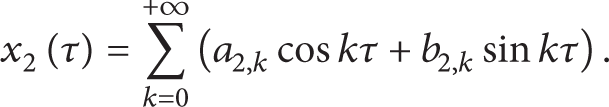
Assuming the periodic solution of systems (2a) and (2b) can be represented by the basis function {cos⁡(kτ), sin(kτ) ∣ k = 0, 1, 2, …}

$x_{\mathrm{1}}\left(\tau \right)={{\displaystyle \sum }}_{k=\mathrm{0}}^{+\infty }\left(a_{\mathrm{1},k}\cos k\tau +b_{\mathrm{1},k}\sin k\tau \right),$

(4a)

$x_{\mathrm{2}}\left(\tau \right)={{\displaystyle \sum }}_{k=\mathrm{0}}^{+\infty }\left(a_{\mathrm{2},k}\cos k\tau +b_{\mathrm{2},k}\sin k\tau \right).$

(4b)

For the initial guess solution, we set

$x_{\mathrm{1},\mathrm{0}}\left(\tau \right)=a_{\mathrm{0}}\cos \tau +b_{\mathrm{0}}\sin \tau ,\hspace{1em}\hspace{1em}{x}_{\mathrm{2},\mathrm{0}}\left(\tau \right)=c_{\mathrm{0}}\cos \tau ,$

(5)

and the auxiliary linear operator is expressed as

$L\left(\begin{array}{c}{\Phi }_{\mathrm{1}}\left(\tau ,q\right)\\ {\Phi }_{\mathrm{2}}\left(\tau ,q\right)\end{array}\right)={\omega }_{\mathrm{0}}^{\mathrm{2}}\left(\begin{array}{c}\frac{{\partial }^2{\Phi }_{\mathrm{1}}\left(\tau ,q\right)}{\partial {\tau }^{\mathrm{2}}}+{\Phi }_{\mathrm{1}}\left(\tau ,q\right)\\ \frac{{\partial }^2{\Phi }_{\mathrm{2}}\left(\tau ,q\right)}{\partial {\tau }^{\mathrm{2}}}+{\Phi }_{\mathrm{2}}\left(\tau ,q\right)\end{array}\right).$

(6)

According to the systems (2a) and (2b), nonlinear operator is defined as follows:

$N\left(\begin{array}{c}{\Phi }_{\mathrm{1}}\left(\tau ,q\right)\\ {\Phi }_{\mathrm{2}}\left(\tau ,q\right)\end{array}\right)=\left(\begin{array}{c}{\Omega }^{\mathrm{2}}\left(q\right)\frac{{\partial }^2{\Phi }_{\mathrm{1}}\left(\tau ,q\right)}{\partial {\tau }^{\mathrm{2}}}+\Omega \left(q\right){\alpha }_{\mathrm{1}}\left[{\Phi }_{\mathrm{1}}^{\mathrm{2}}\left(\tau ,q\right)-\mathrm{1}\right]\frac{\partial {\Phi }_{\mathrm{1}}\left(\tau ,q\right)}{\partial \tau }+{\beta }_{\mathrm{1}}{\Phi }_{\mathrm{1}}\left(\tau ,q\right)\\ \hspace{1em}+{\delta }_{\mathrm{1}}{\Phi }_{\mathrm{1}}^{\mathrm{3}}\left(\tau ,q\right)+{\gamma }_{\mathrm{1}}\left[{\Phi }_{\mathrm{1}}^{\mathrm{3}}\left(\tau ,q\right)-{\Phi }_{\mathrm{2}}^{\mathrm{3}}\left(\tau ,q\right)\right]\\ {\Omega }^{\mathrm{2}}\left(q\right)\frac{{\partial }^2{\Phi }_{\mathrm{2}}\left(\tau ,q\right)}{\partial {\tau }^{\mathrm{2}}}+\Omega \left(q\right){\alpha }_{\mathrm{2}}\left[{\Phi }_{\mathrm{2}}^{\mathrm{2}}\left(\tau ,q\right)-\mathrm{1}\right]\frac{\partial {\Phi }_{\mathrm{2}}\left(\tau ,q\right)}{\partial \tau }+{\beta }_{\mathrm{2}}{\Phi }_{\mathrm{2}}\left(\tau ,q\right)\\ \hspace{1em}+{\delta }_{\mathrm{2}}{\Phi }_{\mathrm{2}}^{\mathrm{3}}\left(\tau ,q\right)+{\gamma }_{\mathrm{2}}\left[{\Phi }_{\mathrm{2}}^{\mathrm{3}}\left(\tau ,q\right)-{\Phi }_{\mathrm{1}}^{\mathrm{3}}\left(\tau ,q\right)\right]\end{array}\right).$

(7)

Taking H(t) = 1, the zero-order deformation equation can be written as

$\left(\mathrm{1}-q\right)L\left(\begin{array}{c}{\Phi }_{\mathrm{1}}(\tau ,q)-x_{\mathrm{1},\mathrm{0}}\left(\tau \right)\\ {\Phi }_{\mathrm{2}}(\tau ,q)-x_{\mathrm{2},\mathrm{0}}\left(\tau \right)\end{array}\right)=q\hslash N\left(\begin{array}{c}{\Phi }_{\mathrm{1}}(\tau ,q)\\ {\Phi }_{\mathrm{2}}(\tau ,q)\end{array}\right),$

(8)

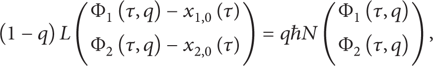
with the initial conditions

${\Phi }_{\mathrm{1}}(\mathrm{0},q)=a\left(q\right),\hspace{1em}\hspace{1em}{\frac{\partial {\Phi }_{\mathrm{1}}(\tau ,q)}{\partial \tau }|}_{\tau =\mathrm{0}}=b\left(q\right),$

(9a)

${\Phi }_{\mathrm{2}}(\mathrm{0},q)=c\left(q\right),\hspace{1em}\hspace{1em}{\frac{\partial {\Phi }_{\mathrm{2}}(\tau ,q)}{\partial \tau }|}_{\tau =\mathrm{0}}=\mathrm{0}.$

(9b)

When q = 0, (8), (9a), and (9b) have solutions

$\begin{array}{c}{\Phi }_{\mathrm{1}}\left(\tau ,\mathrm{0}\right)=x_{\mathrm{1},\mathrm{0}}\left(\tau \right),\hspace{1em}\hspace{1em}{\Phi }_{\mathrm{2}}\left(\tau ,\mathrm{0}\right)=x_{\mathrm{2},\mathrm{0}}\left(\tau \right),\\ \Omega \left(\mathrm{0}\right)={\omega }_{\mathrm{0}}.\end{array}$

(10)

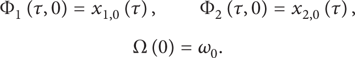
When q = 1, the zero-order deformation equations (8), (9a), and (9b) are equivalent to the original equations (2a), (2b), and (3), so

$\begin{array}{c}{\Phi }_{\mathrm{1}}\left(\tau ,\mathrm{1}\right)=x_{\mathrm{1}}\left(\tau \right),\hspace{1em}\hspace{1em}{\Phi }_{\mathrm{2}}\left(\tau ,\mathrm{1}\right)=x_{\mathrm{2}}\left(\tau \right),\\ \Omega \left(\mathrm{1}\right)=\omega .\end{array}$

(11)

When the embedded variable q increases from 0 to 1, Φ _i (τ,q) changes from the initial guess solution x_i,0(τ) to an unknown exact solution x _i (τ) (i = 1, 2). Likewise, Ω(q) changes from an initial guess frequency ω₀ to the physical frequency ω.

Using Taylor expansion theorem and (10), we get

${\Phi }_{\mathrm{1}}\left(\tau ,q\right)=x_{\mathrm{1},\mathrm{0}}\left(\tau \right)+{{\displaystyle \sum }}_{m=\mathrm{1}}^{+\infty }{x}_{\mathrm{1},m}\left(\tau \right)q^m,$

(12a)

${\Phi }_{\mathrm{2}}\left(\tau ,q\right)=x_{\mathrm{2},\mathrm{0}}\left(\tau \right)+{{\displaystyle \sum }}_{m=\mathrm{1}}^{+\infty }{x}_{\mathrm{2},m}\left(\tau \right)q^m,$

(12b)

$\Omega \left(q\right)={\omega }_{\mathrm{0}}+{{\displaystyle \sum }}_{m=\mathrm{1}}^{+\infty }{\omega }_m{q}^m,$

(12c)

${x_{\mathrm{1},m}\left(\tau \right)=\frac{\mathrm{1}}{m!}\frac{{\partial }^m{\Phi }_{\mathrm{1}}\left(\tau ,q\right)}{\partial q^m}|}_{q=\mathrm{0}},$

(13a)

${x_{\mathrm{2},m}\left(\tau \right)=\frac{\mathrm{1}}{m!}\frac{{\partial }^m{\Phi }_{\mathrm{2}}\left(\tau ,q\right)}{\partial q^m}|}_{q=\mathrm{0}},$

(13b)

${{\omega }_m=\frac{\mathrm{1}}{m!}\frac{{\partial }^m\Omega \left(q\right)}{\partial q^m}|}_{q=\mathrm{0}}.$

(13c)

Assuming that the auxiliary parameter ℏ is selected appropriately, (12a), (12b), and (12c)'s power series are converging when q = 1. By (13a), (13b), and (13c), we get the series solution

$x_{\mathrm{1}}\left(\tau \right)=x_{\mathrm{1},\mathrm{0}}\left(\tau \right)+{{\displaystyle \sum }}_{m=\mathrm{1}}^{+\infty }{x}_{\mathrm{1},m}\left(\tau \right),$

(14a)

$x_{\mathrm{2}}\left(\tau \right)=x_{\mathrm{2},\mathrm{0}}\left(\tau \right)+{{\displaystyle \sum }}_{m=\mathrm{1}}^{+\infty }{x}_{\mathrm{2},m}\left(\tau \right),$

(14b)

$\omega ={\omega }_{\mathrm{0}}+{{\displaystyle \sum }}_{m=\mathrm{1}}^{+\infty }{\omega }_m.$

(14c)

For convenience, we define the vector as follows:

${\mathbf{x}}_{\mathrm{1},n}=\left\{x_{\mathrm{1},\mathrm{0}}\left(\tau \right),x_{\mathrm{1},\mathrm{1}}\left(\tau \right),\dots ,x_{\mathrm{1},n}\left(\tau \right)\right\},$

(15a)

${\mathbf{x}}_{\mathrm{2},n}=\left\{x_{\mathrm{2},\mathrm{0}}\left(\tau \right),x_{\mathrm{2},\mathrm{1}}\left(\tau \right),\dots ,x_{\mathrm{2},n}\left(\tau \right)\right\},$

(15b)

${\mathbf{\omega }}_n=\left\{{\omega }_{\mathrm{0}},{\omega }_{\mathrm{1}},\dots ,{\omega }_n\right\}.$

(15c)

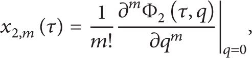
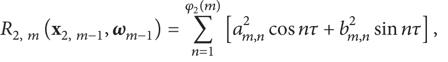
By differentiating the zeroth-order deformation equation (8) m times with respect to q, and both sides of the resulting equation are divided by m!, and assume q = 0; we obtain m order deformation equation

$L\left(\begin{array}{c}{x}_{\mathrm{1},\mathrm{\hspace{0.17em}\hspace{0.17em}}m}\left(\tau \right)-{\chi }_m{x}_{\mathrm{1},\mathrm{\hspace{0.17em}\hspace{0.17em}}m-\mathrm{1}}\left(\tau \right)\\ x_{\mathrm{2},\mathrm{\hspace{0.17em}\hspace{0.17em}}m}\left(\tau \right)-{\chi }_m{x}_{\mathrm{2},\mathrm{\hspace{0.17em}\hspace{0.17em}}m-\mathrm{1}}\left(\tau \right)\end{array}\right)=\hslash \left(\begin{array}{c}{R}_{\mathrm{1},\mathrm{\hspace{0.17em}\hspace{0.17em}}m}({\mathbf{x}}_{\mathrm{1},\mathrm{\hspace{0.17em}\hspace{0.17em}}m-\mathrm{1}},{\mathbf{\omega }}_{m-\mathrm{1}})\\ R_{\mathrm{2},\mathrm{\hspace{0.17em}\hspace{0.17em}}m}({\mathbf{x}}_{\mathrm{2},\mathrm{\hspace{0.17em}\hspace{0.17em}}m-\mathrm{1}},{\mathbf{\omega }}_{m-\mathrm{1}})\end{array}\right),$

(16)

with the initial conditions

$\begin{array}{c}{x}_{\mathrm{1},\mathrm{\hspace{0.17em}\hspace{0.17em}}m}\left(\mathrm{0}\right)=a_m,\hspace{1em}\hspace{1em}{x}_{\mathrm{1},\mathrm{\hspace{0.17em}\hspace{0.17em}}m}^{\prime }\left(\mathrm{0}\right)=b_m,x_{\mathrm{2},\mathrm{\hspace{0.17em}\hspace{0.17em}}m}\left(\mathrm{0}\right)=c_m,\hspace{1em}{x}_{\mathrm{2},\mathrm{\hspace{0.17em}\hspace{0.17em}}m}^{\prime }\left(\mathrm{0}\right)=\mathrm{0},\hspace{1em}\left(m\ge \mathrm{1}\right),\\ \left(\begin{array}{c}{R}_{\mathrm{1},\mathrm{\hspace{0.17em}\hspace{0.17em}}m}\left({\mathbf{x}}_{\mathrm{1},\mathrm{\hspace{0.17em}\hspace{0.17em}}m-\mathrm{1}},{\mathbf{\omega }}_{m-\mathrm{1}}\right)\\ R_{\mathrm{2},\mathrm{\hspace{0.17em}\hspace{0.17em}}m}\left({\mathbf{x}}_{\mathrm{2},\mathrm{\hspace{0.17em}\hspace{0.17em}}m-\mathrm{1}},{\mathbf{\omega }}_{m-\mathrm{1}}\right)\end{array}\right)=\frac{\mathrm{1}}{\left(m-\mathrm{1}\right)!}{\frac{{\partial }^{m-\mathrm{1}}N\left(\begin{array}{c}{\Phi }_{\mathrm{1}}\left(\tau ,q\right)\\ {\Phi }_{\mathrm{2}}\left(\tau ,q\right)\end{array}\right)}{\partial q^{m-\mathrm{1}}}|}_{q=\mathrm{0}}.\end{array}$

(17)

According to the solution expression principles and the definition of linear operator L, by (16), we obtained solutions x_1,m(τ) and x_2,m(τ) without secular terms τsinτ and τcos⁡τ. The right-hand side of (16) cannot contain sinτ, cos⁡τ, or similar items. We set the coefficient of these items are 0, and we get

$\frac{\mathrm{1}}{\pi }{{\displaystyle \int }}_{\mathrm{0}}^{\mathrm{2}\pi }{R}_{\mathrm{1},\mathrm{\hspace{0.17em}\hspace{0.17em}}m}\left({\mathbf{x}}_{\mathrm{1},\mathrm{\hspace{0.17em}\hspace{0.17em}}m-\mathrm{1}},{\mathbf{\omega }}_{m-\mathrm{1}}\right)\cos \tau \hspace{0.17em}\text{d}\tau =\mathrm{0},$

(18a)

$\frac{\mathrm{1}}{\pi }{{\displaystyle \int }}_{\mathrm{0}}^{\mathrm{2}\pi }{R}_{\mathrm{2},\mathrm{\hspace{0.17em}\hspace{0.17em}}m}\left({\mathbf{x}}_{\mathrm{2},\mathrm{\hspace{0.17em}\hspace{0.17em}}m-\mathrm{1}},{\mathbf{\omega }}_{m-\mathrm{1}}\right)\cos \tau \hspace{0.17em}\text{d}\tau =\mathrm{0},$

(18b)

$\frac{\mathrm{1}}{\pi }{{\displaystyle \int }}_{\mathrm{0}}^{\mathrm{2}\pi }{R}_{\mathrm{1},\mathrm{\hspace{0.17em}\hspace{0.17em}}m}\left({\mathbf{x}}_{\mathrm{1},\mathrm{\hspace{0.17em}\hspace{0.17em}}m-\mathrm{1}},{\mathbf{\omega }}_{m-\mathrm{1}}\right)\sin \tau \hspace{0.17em}\text{d}\tau =\mathrm{0},$

(18c)

$\frac{\mathrm{1}}{\pi }{{\displaystyle \int }}_{\mathrm{0}}^{\mathrm{2}\pi }{R}_{\mathrm{2},\mathrm{\hspace{0.17em}\hspace{0.17em}}m}\left({\mathbf{x}}_{\mathrm{2},\mathrm{\hspace{0.17em}\hspace{0.17em}}m-\mathrm{1}},{\mathbf{\omega }}_{m-\mathrm{1}}\right)\sin \tau \hspace{0.17em}\text{d}\tau =\mathrm{0}.$

(18d)

Then

$R_{\mathrm{1},\mathrm{\hspace{0.17em}\hspace{0.17em}}m}\left({\mathbf{x}}_{\mathrm{1},\mathrm{\hspace{0.17em}\hspace{0.17em}}m-\mathrm{1}},{\mathbf{\omega }}_{m-\mathrm{1}}\right)={\displaystyle \sum }_{n=\mathrm{1}}^{{\phi }_{\mathrm{1}}\left(m\right)}\left[a_{m,n}^{\mathrm{1}}\cos n\tau +b_{m,n}^{\mathrm{1}}\sin n\tau \right],$

(19a)

$R_{\mathrm{2},\mathrm{\hspace{0.17em}\hspace{0.17em}}m}\left({\mathbf{x}}_{\mathrm{2},\mathrm{\hspace{0.17em}\hspace{0.17em}}m-\mathrm{1}},{\mathbf{\omega }}_{m-\mathrm{1}}\right)={\displaystyle \sum }_{n=\mathrm{1}}^{{\phi }_{\mathrm{2}}\left(m\right)}\left[a_{m,n}^{\mathrm{2}}\cos n\tau +b_{m,n}^{\mathrm{2}}\sin n\tau \right],$

(19b)

$a_{m,\mathrm{\hspace{0.17em}\hspace{0.17em}}n}^{\mathrm{1}}=\frac{\mathrm{1}}{\pi }{{\displaystyle \int }}_{\mathrm{0}}^{\mathrm{2}\pi }{R}_{\mathrm{1},\mathrm{\hspace{0.17em}\hspace{0.17em}}m}\left({\mathbf{x}}_{\mathrm{1},\mathrm{\hspace{0.17em}\hspace{0.17em}}m-\mathrm{1}},{\mathbf{\omega }}_{m-\mathrm{1}}\right)\cos \left(n\tau \right)\text{d}\tau ,$

(20a)

$a_{m,\mathrm{\hspace{0.17em}\hspace{0.17em}}n}^{\mathrm{2}}=\frac{\mathrm{1}}{\pi }{{\displaystyle \int }}_{\mathrm{0}}^{\mathrm{2}\pi }{R}_{\mathrm{2},\mathrm{\hspace{0.17em}\hspace{0.17em}}m}\left({\mathbf{x}}_{\mathrm{2},\mathrm{\hspace{0.17em}\hspace{0.17em}}m-\mathrm{1}},{\mathbf{\omega }}_{m-\mathrm{1}}\right)\cos \left(n\tau \right)\text{d}\tau ,$

(20b)

$b_{m,\mathrm{\hspace{0.17em}\hspace{0.17em}}n}^{\mathrm{1}}=\frac{\mathrm{1}}{\pi }{{\displaystyle \int }}_{\mathrm{0}}^{\mathrm{2}\pi }{R}_{\mathrm{1},\mathrm{\hspace{0.17em}\hspace{0.17em}}m}\left({\mathbf{x}}_{\mathrm{1},\mathrm{\hspace{0.17em}\hspace{0.17em}}m-\mathrm{1}},{\mathbf{\omega }}_{m-\mathrm{1}}\right)\sin \left(n\tau \right)\text{d}\tau ,$

(20c)

$b_{m,\mathrm{\hspace{0.17em}\hspace{0.17em}}n}^{\mathrm{2}}=\frac{\mathrm{1}}{\pi }{{\displaystyle \int }}_{\mathrm{0}}^{\mathrm{2}\pi }{R}_{\mathrm{2},\mathrm{\hspace{0.17em}\hspace{0.17em}}m}\left({\mathbf{x}}_{\mathrm{2},\mathrm{\hspace{0.17em}\hspace{0.17em}}m-\mathrm{1}},{\mathbf{\omega }}_{m-\mathrm{1}}\right)\sin \left(n\tau \right)\text{d}\tau .$

(20d)

Using (16), (18a), (18b), (18c), and (18d), we can gradually get ω _k , a _k , b _k , and c _k (k = 0, 1, 2, …).

3. Numerical Simulation

In this section, we get the periodic solution of systems (1a) and (1b) by HAM under the condition of the given parameters α _i , β _i , γ _i , and δ _i (i = 1, 2). First we consider the case α₁≠α₂; take α₁ = 1, α₂ = 99/100, β₁ = β₂ = 1, γ₁ = γ₂ = 1, δ₁ = δ₂ = 1, and then put them into (18a), (18b), (18c), and (18d); we can get the following nonlinear algebraic equations:

$\mathrm{6}{a}_{\mathrm{0}}^{\mathrm{3}}-\mathrm{3}{c}_{\mathrm{0}}^{\mathrm{3}}+a_{\mathrm{0}}^{\mathrm{2}}{b}_{\mathrm{0}}{\omega }_{\mathrm{0}}+b_{\mathrm{0}}\left(-\mathrm{4}+b_{\mathrm{0}}^{\mathrm{2}}\right){\omega }_{\mathrm{0}}+a_{\mathrm{0}}\left(\mathrm{4}+\mathrm{6}{b}_{\mathrm{0}}^{\mathrm{2}}-\mathrm{4}{\omega }_{\mathrm{0}}^{\mathrm{2}}\right)=\mathrm{0},$

(21a)

$\mathrm{6}{b}_{\mathrm{0}}^{\mathrm{3}}-a_{\mathrm{0}}\left(-\mathrm{4}+a_{\mathrm{0}}^{\mathrm{2}}\right){\omega }_{\mathrm{0}}-a_{\mathrm{0}}{b_{\mathrm{0}}^{\mathrm{2}}\omega }_{\mathrm{0}}+b_{\mathrm{0}}\left(\mathrm{4}+\mathrm{6}{a}_{\mathrm{0}}^{\mathrm{2}}-\mathrm{4}{\omega }_{\mathrm{0}}^{\mathrm{2}}\right)=\mathrm{0},$

(21b)

$-\mathrm{3}{a}_{\mathrm{0}}^{\mathrm{3}}-\mathrm{3}{a}_{\mathrm{0}}{b}_{\mathrm{0}}^{\mathrm{2}}+\mathrm{4}{c}_{\mathrm{0}}+\mathrm{6}{c}_{\mathrm{0}}^{\mathrm{3}}-\mathrm{4}{c}_{\mathrm{0}}{\omega }_{\mathrm{0}}^{\mathrm{2}}=\mathrm{0},$

(21c)

$\mathrm{100}{a}_{\mathrm{0}}^{\mathrm{2}}{b}_{\mathrm{0}}+\mathrm{100}{b}_{\mathrm{0}}^{\mathrm{3}}+\mathrm{33}{c}_{\mathrm{0}}\left(-\mathrm{4}+c_{\mathrm{0}}^{\mathrm{2}}\right){\omega }_{\mathrm{0}}=\mathrm{0}.$

(21d)

Solve the equations; we have a₀ = 2, b₀ = 0, c₀ = 2, and ω₀ = 2.

Next make use of the relationship between frequency ω and parameter ℏ to determine the value range of ℏ. Figure 1 is the curve of ω-ℏ by the fourth-order approximation; when − 0.28 < ℏ < − 0.18, the series of ω is convergent. The selection of different auxiliary parameters ℏ can improve the accuracy of the final series solution; for simplicity, take ℏ = − 0.2.

Figure 1:

The fourth-order approximation curve of ω versus ℏ.

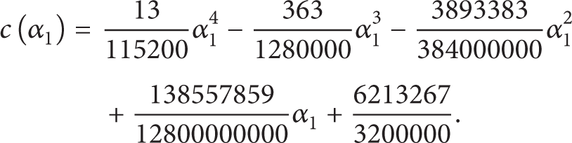
We further explore the relationship between the frequency, amplitude, and the parameters. According to (3), the amplitudes of the two components x₁(t), x₂(t) are a, c in periodic solution of the system. In this example, since α₁≠α₂ and other parameter values are the same, the focus of the research is the relationship between ω, a, c and α₁, α₂. First, set α₁ as an unknown parameter, and set α₂ as a known quantity (α₂ = 99/100). According to the HAM, the second-order approximate expression of ω(α₁), a(α₁), and c(α₁) can be written, respectively, as follows:

$\omega \left({\alpha }_{\mathrm{1}}\right)=\frac{\mathrm{44779}}{\mathrm{256000000}}{\alpha }_{\mathrm{1}}^{\mathrm{4}}-\frac{\mathrm{1731873}}{\mathrm{6400000000}}{\alpha }_{\mathrm{1}}^{\mathrm{3}}-\frac{\mathrm{23516728323}}{\mathrm{1280000000000}}{\alpha }_{\mathrm{1}}^{\mathrm{2}}+\frac{\mathrm{986875659}}{\mathrm{102400000000}}{\alpha }_{\mathrm{1}}+\frac{\mathrm{78481134113267}}{\mathrm{40960000000000}},$

(22a)

$a\left({\alpha }_{\mathrm{1}}\right)=-\frac{\mathrm{121}}{\mathrm{4000000}}{\alpha }_{\mathrm{1}}^{\mathrm{4}}+\frac{\mathrm{714791}}{\mathrm{800000000}}{\alpha }_{\mathrm{1}}^{\mathrm{3}}-\frac{\mathrm{2575699901}}{\mathrm{240000000000}}{\alpha }_{\mathrm{1}}^{\mathrm{2}}+\frac{\mathrm{81116409}}{\mathrm{2560000000}}{\alpha }_{\mathrm{1}}+\frac{\mathrm{2458329452757}}{\mathrm{1280000000000}},$

(22b)

$c\left({\alpha }_{\mathrm{1}}\right)=\frac{\mathrm{13}}{\mathrm{115200}}{\alpha }_{\mathrm{1}}^{\mathrm{4}}-\frac{\mathrm{363}}{\mathrm{1280000}}{\alpha }_{\mathrm{1}}^{\mathrm{3}}-\frac{\mathrm{3893383}}{\mathrm{384000000}}{\alpha }_{\mathrm{1}}^{\mathrm{2}}+\frac{\mathrm{138557859}}{\mathrm{12800000000}}{\alpha }_{\mathrm{1}}+\frac{\mathrm{6213267}}{\mathrm{3200000}}.$

(22c)

Then set α₂ as an unknown parameter, α₁ as a known quantity (α₁ = 1); the second-order approximate expression of ω(α₂), a(α₂), and c(α₂) can be written, respectively, as follows:

$\omega \left({\alpha }_{\mathrm{2}}\right)=\frac{\mathrm{1937}}{\mathrm{11059200}}{\alpha }_{\mathrm{2}}^{\mathrm{4}}-\frac{\mathrm{757}}{\mathrm{2764800}}{\alpha }_{\mathrm{2}}^{\mathrm{3}}-\frac{\mathrm{101519}}{\mathrm{5529600}}{\alpha }_{\mathrm{2}}^{\mathrm{2}}+\frac{\mathrm{2989}}{\mathrm{307200}}{\alpha }_{\mathrm{2}}+\frac{\mathrm{784659}}{\mathrm{409600}},$

(23a)

$a\left({\alpha }_{\mathrm{2}}\right)=\frac{\mathrm{17}}{\mathrm{207360}}{\alpha }_{\mathrm{2}}^{\mathrm{4}}+\frac{\mathrm{919}}{\mathrm{1036800}}{\alpha }_{\mathrm{2}}^{\mathrm{3}}-\frac{\mathrm{23207}}{\mathrm{1036800}}{\alpha }_{\mathrm{2}}^{\mathrm{2}}+\frac{\mathrm{3691}}{\mathrm{115200}}{\alpha }_{\mathrm{2}}+\frac{\mathrm{1159}}{\mathrm{600}},$

(23b)

$c\left({\alpha }_{\mathrm{2}}\right)=-\frac{\mathrm{31}}{\mathrm{115200}}{\alpha }_{\mathrm{2}}^{\mathrm{3}}+\frac{\mathrm{19}}{\mathrm{12800}}{\alpha }_{\mathrm{2}}^{\mathrm{2}}+\frac{\mathrm{419}}{\mathrm{38400}}{\alpha }_{\mathrm{2}}+\frac{\mathrm{44471}}{\mathrm{23040}}.$

(23c)

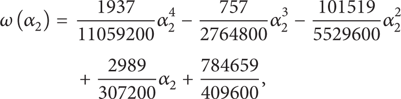
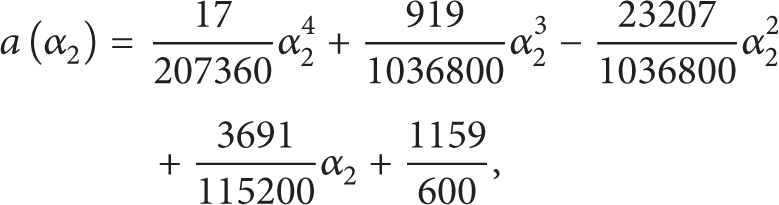
Figure 2 shows the image of ω(α₁) and ω(α₂) drawn in the same Cartesian coordinate system, namely, the curves of ω-α₁ and ω-α₂.

Figure 2:

The second-order approximation curves of ω-α₁ and ω-α₂.

One can see from Figure 2 that if α₁, α₂ are within the suitable range (− 1/2 < α₁, α₂ < 3/2), and the gap between α₁ and α₂ is very small (|α₁ − α₂| < 1/50), then the approximate value of frequency ω can be stabilized in the vicinity of 1.9. Thus it can be seen that the setting of α₁, α₂ in this example is reasonable.

Figures 3 and 4 give the fourth-order analytical approximate phase diagram and time history curve, respectively. The fourth-order analytical approximation agrees well with the solution obtained by the numerical integration method. Here the initial conditions that numerical integration method meets are x₁(0) = 2, x₁′(0) = 0, x₂(0) = 2, and x₂′(0) = 0.

Figure 3:

Comparison of the phase portrait curves of the fourth-order approximation with the numerical integration method.

Figure 4:

Comparison of the time history responses s of the fourth-order approximation with the numerical integration method.

The specific expressions of the fourth-order analytical approximate that the systems (1a) and (1b) satisfy the above initial conditions are

$x_{\mathrm{1}}\left(t\right)=\mathrm{1.84957290}\cos \omega t+\mathrm{0.32613610}\sin \omega t+\mathrm{0.09496963}\cos \mathrm{3}\omega t-\mathrm{0.08934836}\sin \mathrm{3}\omega t-\mathrm{0.00426108}\cos \mathrm{5}\omega t-\mathrm{0.01258828}\sin \mathrm{5}\omega t-\mathrm{0.00140884}\cos \mathrm{7}\omega t+\mathrm{0.00008743}\sin \mathrm{7}\omega t+\mathrm{0.00002442}\cos \mathrm{9}\omega t+\mathrm{0.00009499}\sin \mathrm{9}\omega t,$

(24a)

$x_{\mathrm{2}}\left(t\right)=\mathrm{1.84958869}\cos \omega t+\mathrm{0.32448489}\sin \omega t+\mathrm{0.09453651}\cos \mathrm{3}\omega t-\mathrm{0.08812457}\sin \mathrm{3}\omega t-\mathrm{0.00411388}\cos \mathrm{5}\omega t-\mathrm{0.01230200}\sin \mathrm{5}\omega t-\mathrm{0.00135866}\cos \mathrm{7}\omega t+\mathrm{0.00008301}\sin \mathrm{7}\omega t+\mathrm{0.00002371}\cos \mathrm{9}\omega t+\mathrm{0.00009085}\sin \mathrm{9}\omega t,$

(24b)

where

$\omega =\mathrm{1.90070426}.$

(24c)

Now consider the case of β₁≠β₂. Taking each parameter as α₁ = α₂ = 1, β₁ = 1, β₂ = 999/1000, γ₁ = γ₂ = 1, and δ₁ = δ₂ = 1; in accordance with the method of the previous example, put them into (18a), (18b), (18c), and (18d), and obtain the following nonlinear algebraic equations:

$\mathrm{6}{a}_{\mathrm{0}}^{\mathrm{3}}-\mathrm{3}{c}_{\mathrm{0}}^{\mathrm{3}}+a_{\mathrm{0}}^{\mathrm{2}}{b}_{\mathrm{0}}{\omega }_{\mathrm{0}}+b_{\mathrm{0}}\left(-\mathrm{4}+b_{\mathrm{0}}^{\mathrm{2}}\right){\omega }_{\mathrm{0}}+a_{\mathrm{0}}\left(\mathrm{4}+\mathrm{6}{b}_{\mathrm{0}}^{\mathrm{2}}-\mathrm{4}{\omega }_{\mathrm{0}}^{\mathrm{2}}\right)=\mathrm{0},$

(25a)

$\mathrm{6}{b}_{\mathrm{0}}^{\mathrm{3}}-a_{\mathrm{0}}\left(-\mathrm{4}+a_{\mathrm{0}}^{\mathrm{2}}\right){\omega }_{\mathrm{0}}-a_{\mathrm{0}}{b_{\mathrm{0}}^{\mathrm{2}}\omega }_{\mathrm{0}}+b_{\mathrm{0}}\left(\mathrm{4}+\mathrm{6}{a}_{\mathrm{0}}^{\mathrm{2}}-\mathrm{4}{\omega }_{\mathrm{0}}^{\mathrm{2}}\right)=\mathrm{0},$

(25b)

$-\mathrm{750}{a}_{\mathrm{0}}^{\mathrm{3}}-\mathrm{750}{a}_{\mathrm{0}}{b}_{\mathrm{0}}^{\mathrm{2}}+\mathrm{999}{c}_{\mathrm{0}}+\mathrm{1500}{c}_{\mathrm{0}}^{\mathrm{3}}-\mathrm{1000}{c}_{\mathrm{0}}{\omega }_{\mathrm{0}}^{\mathrm{2}}=\mathrm{0},$

(25c)

$\mathrm{3}{a}_{\mathrm{0}}^{\mathrm{2}}{b}_{\mathrm{0}}+\mathrm{3}{b}_{\mathrm{0}}^{\mathrm{3}}+c_{\mathrm{0}}(-\mathrm{4}+c_{\mathrm{0}}^{\mathrm{2}}){\omega }_{\mathrm{0}}=\mathrm{0}.$

(25d)

Solving the equations, obtained a₀ = 2, b₀ = 0, c₀ = 2, and ω₀ = 2.

Using the relationship between the frequency ω and the parameters ℏ is to determine the range of ℏ. Figure 5 is the curve of ω-ℏ by the third-order approximation; as can be seen from the figure, when − 0.28 < ℏ < − 0.18, the series of ω is convergent. For simplicity, take ℏ = − 0.1.

Figure 5:

The third-order approximation curve of ω versus ℏ.

Since β₁≠β₂, based on the idea of the previous example, we focus on studying the relationship between ω, a, c and the parameters β₁, β₂. First, set β₁ as an unknown parameter, β₂ as a known amount (β₂ = 999/1000); in accordance with the HAM the second-order approximate expression of ω(β₁), a(β₁), and c(β₁) can be written as

$\omega \left({\beta }_{\mathrm{1}}\right)=\mathrm{2}+\frac{\mathrm{1}}{\mathrm{320000000}\left(\mathrm{117997}+\mathrm{25000}{\beta }_{\mathrm{1}}+\mathrm{1000}{\beta }_{\mathrm{1}}^{\mathrm{2}}\right)}\times (\mathrm{3000000000}{\beta }_{\mathrm{1}}^{\mathrm{3}}+\mathrm{44982001}\pi {\beta }_{\mathrm{1}}^{\mathrm{2}}-\mathrm{237995998000}{\beta }_{\mathrm{1}}^{\mathrm{2}}+\mathrm{341802016}\pi {\beta }_{\mathrm{1}}-\mathrm{1683662968000}{\beta }_{\mathrm{1}}-\mathrm{387215972}\pi +\mathrm{48498065000}),$

(26a)

$a\left({\beta }_{\mathrm{1}}\right)=\mathrm{2}-\frac{\mathrm{1}}{\mathrm{40000000}\left(\mathrm{11797}+\mathrm{25000}{\beta }_{\mathrm{1}}+\mathrm{1000}{\beta }_{\mathrm{1}}^{\mathrm{2}}\right)}\times (\mathrm{2000000000}{\beta }_{\mathrm{1}}^{\mathrm{3}}+\mathrm{6000000000}{\beta }_{\mathrm{1}}^{\mathrm{2}}-\mathrm{71973001}\pi {\beta }_{\mathrm{1}}+\mathrm{24004998000}{\beta }_{\mathrm{1}}+\mathrm{72044998}\pi +\mathrm{112006996000}),$

(26b)

$c\left({\beta }_{\mathrm{1}}\right)=\mathrm{2}+\frac{\mathrm{1}}{\mathrm{40000}\left(\mathrm{11797}+\mathrm{25000}{\beta }_{\mathrm{1}}+\mathrm{1000}{\beta }_{\mathrm{1}}^{\mathrm{2}}\right)}\times (\mathrm{2999}\pi {\beta }_{\mathrm{1}}^{\mathrm{2}}+\mathrm{5000000}{\beta }_{\mathrm{1}}^{\mathrm{2}}+\mathrm{65975}\pi {\beta }_{\mathrm{1}}-\mathrm{22000000}{\beta }_{\mathrm{1}}-\mathrm{69046}\pi -\mathrm{126982006}).$

(26c)

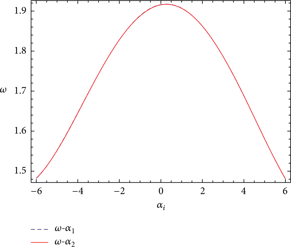
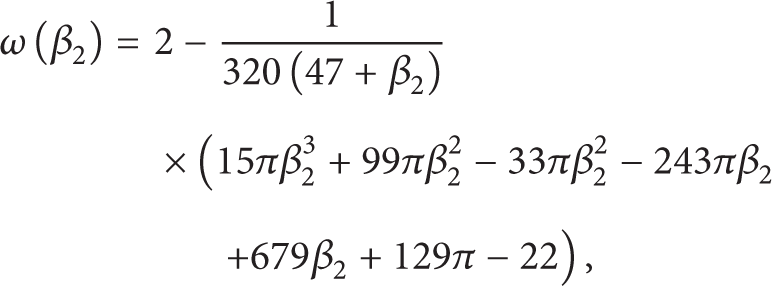
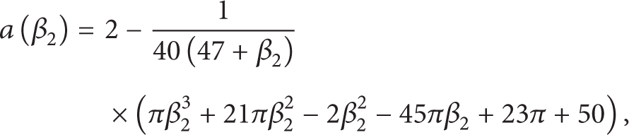
Next, set β₂ as an unknown parameter, β₁ as an known quantity (β₁ = 1); the second-order approximate expression of ω(β₂), a(β₂), and c(β₂) can be, respectively, written as

$\omega \left({\beta }_{\mathrm{2}}\right)=\mathrm{2}-\frac{\mathrm{1}}{\mathrm{320}\left(\mathrm{47}+{\beta }_{\mathrm{2}}\right)}\times (\mathrm{15}\pi {\beta }_{\mathrm{2}}^{\mathrm{3}}+\mathrm{99}\pi {\beta }_{\mathrm{2}}^{\mathrm{2}}-\mathrm{33}\pi {\beta }_{\mathrm{2}}^{\mathrm{2}}-\mathrm{243}\pi {\beta }_{\mathrm{2}}+\mathrm{679}{\beta }_{\mathrm{2}}+\mathrm{129}\pi -\mathrm{22}),$

(27a)

$a\left({\beta }_{\mathrm{2}}\right)=\mathrm{2}-\frac{\mathrm{1}}{\mathrm{40}\left(\mathrm{47}+{\beta }_{\mathrm{2}}\right)}\times \left(\pi {\beta }_{\mathrm{2}}^{\mathrm{3}}+\mathrm{21}\pi {\beta }_{\mathrm{2}}^{\mathrm{2}}-\mathrm{2}{\beta }_{\mathrm{2}}^{\mathrm{2}}-\mathrm{45}\pi {\beta }_{\mathrm{2}}+\mathrm{23}\pi +\mathrm{50}\right),$

(27b)

$c\left({\beta }_{\mathrm{2}}\right)=\mathrm{2}-\frac{\mathrm{1}}{\mathrm{20}\left(\mathrm{47}+{\beta }_{\mathrm{2}}\right)}\times \left(\mathrm{12}\pi {\beta }_{\mathrm{2}}^{\mathrm{2}}+{\beta }_{\mathrm{2}}^{\mathrm{2}}-\mathrm{24}\pi {\beta }_{\mathrm{2}}+{\beta }_{\mathrm{2}}+\mathrm{12}\pi +\mathrm{22}\right).$

(27c)

Draw the image of ω(β₁) and ω(β₂) in the same Cartesian coordinate system; we get curve ω-β₁ and curve ω-β₂, as Figure 6 demonstrates.

Figure 6:

The first-order approximation curves of ω-β₁ and ω-β₂.

Similar to the last case, if β₁, β₂ are within the appropriate range 1/2 < β₁, β₂ < 3/2 and the gap between β₁ and β₂ is very narrow (|β₁ − β₂| < 1/5000), then the frequency ω approximation can be stabilized at 1.95 nearby.

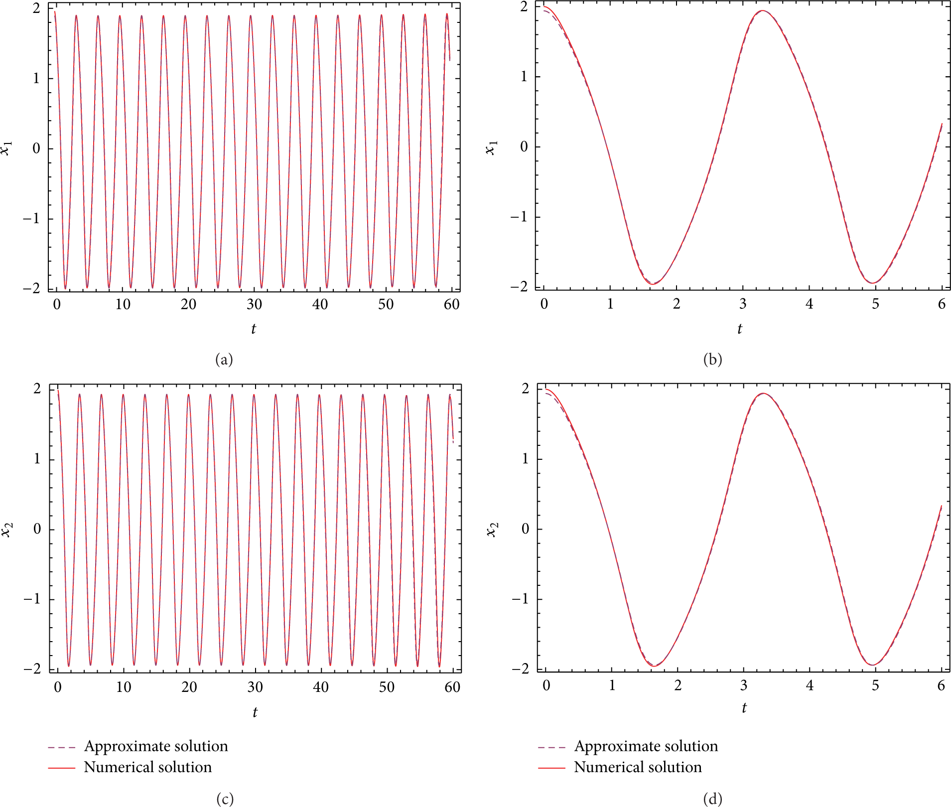
Figures 7 and 8 give the third-order analytical approximate phase diagram, respectively. It is not difficult to find that third-order analytical approximation agrees well with the solution obtained by the numerical integration method. Of course, to get a more accurate solution, we can appropriately increase order of count, in order to increase the number of items series solution; here the initial conditions that numerical integration method meets are x₁(0) = 2, x₁′(0) = 0, x₂(0) = 2, and x₂′(0) = 0.

Figure 7:

Comparison of the phase portrait curves of the third-order approximation with the numerical integration method.

Figure 8:

Comparison of the time history responses of the third-order approximation with the numerical integration method.

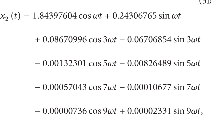
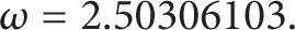
Finally, the third-order analytical approximation (x₁(t),x₂(t),ω) that the systems (1a) and (1b) satisfy the above initial conditions is

$x_{\mathrm{1}}\left(t\right)=\mathrm{1.89282223}\cos \omega t+\mathrm{0.27163323}\sin \omega t+\mathrm{0.06266590}\cos \mathrm{3}\omega t-\mathrm{0.08378610}\sin \mathrm{3}\omega t-\mathrm{0.00331194}\cos \mathrm{5}\omega t-\mathrm{0.00394322}\sin \mathrm{5}\omega t-\mathrm{0.00010233}\cos \mathrm{7}\omega t+\mathrm{0.00006081}\sin \mathrm{7}\omega t,$

(28a)

$x_{\mathrm{2}}\left(t\right)=\mathrm{1.89268859}\cos \omega t+\mathrm{0.27164498}\sin \omega t+\mathrm{0.06274216}\cos \mathrm{3}\omega t-\mathrm{0.08378165}\sin \mathrm{3}\omega t-\mathrm{0.00328250}\cos \mathrm{5}\omega t-\mathrm{0.00394712}\sin \mathrm{5}\omega t-\mathrm{0.00008900}\cos \mathrm{7}\omega t+\mathrm{0.00005956}\sin \mathrm{7}\omega t,$

(28b)

where

$\omega =\mathrm{1.92252889}.$

(28c)

Consider the case of γ₁≠γ₂; take α₁ = α₂ = 1, β₁ = β₂ = 1, γ₁ = 2, γ₂ = 3, and δ₁ = δ₂ = 2 and then put them into (18a), (18b), (18c), and (18d); we obtained the following nonlinear algebraic equations:

$\mathrm{12}{a}_{\mathrm{0}}^{\mathrm{3}}-\mathrm{6}{c}_{\mathrm{0}}^{\mathrm{3}}+a_{\mathrm{0}}^{\mathrm{2}}{b}_{\mathrm{0}}{\omega }_{\mathrm{0}}+b_{\mathrm{0}}\left(-\mathrm{4}+b_{\mathrm{0}}^{\mathrm{2}}\right){\omega }_{\mathrm{0}}+\mathrm{4}{a}_{\mathrm{0}}\left(\mathrm{1}+\mathrm{3}{b}_{\mathrm{0}}^{\mathrm{2}}-\mathrm{4}{\omega }_{\mathrm{0}}^{\mathrm{2}}\right)=\mathrm{0},$

(29a)

$\mathrm{4}{b}_{\mathrm{0}}\left(\mathrm{1}+\mathrm{3}{a}_{\mathrm{0}}^{\mathrm{2}}-\mathrm{3}{b}_{\mathrm{0}}^{\mathrm{2}}\right)-a_{\mathrm{0}}\left(-\mathrm{4}+a_{\mathrm{0}}^{\mathrm{2}}+b_{\mathrm{0}}^{\mathrm{2}}\right){\omega }_{\mathrm{0}}-\mathrm{4}{b}_{\mathrm{0}}{\omega }_{\mathrm{0}}^{\mathrm{2}}=\mathrm{0},$

(29b)

$\mathrm{9}{a}_{\mathrm{0}}^{\mathrm{3}}+\mathrm{9}{a}_{\mathrm{0}}{b}_{\mathrm{0}}^{\mathrm{2}}-\mathrm{4}{c}_{\mathrm{0}}-\mathrm{15}{c}_{\mathrm{0}}^{\mathrm{3}}-\mathrm{4}{c}_{\mathrm{0}}{\omega }_{\mathrm{0}}^{\mathrm{2}}=\mathrm{0},$

(29c)

$\mathrm{9}{a}_{\mathrm{0}}^{\mathrm{2}}{b}_{\mathrm{0}}+\mathrm{9}{b}_{\mathrm{0}}^{\mathrm{3}}+c_{\mathrm{0}}(-\mathrm{4}+c_{\mathrm{0}}^{\mathrm{2}}){\omega }_{\mathrm{0}}=\mathrm{0}.$

(29d)

Solving these equations, we obtained a₀ = 2, b₀ = 0, c₀ = 2, and ${\omega }_0=\sqrt{7}$ .

Utilizing the relationship between frequency ω and parameter ℏ again is to determine the value range of ℏ. Figure 9 is the curve of ω-ℏ by the fourth-order approximation; obviously, when − 0.16 < ℏ < − 0.09, the series of ω is convergent. We may as well select ℏ = − 0.1.

Figure 9:

The fourth-order approximation curve of ω versus ℏ.

In this case, the unequal parameters γ₁, γ₂ are in the coupling, so the relationship between frequency, amplitude, and them becomes relatively simple. Set γ₁, γ₂ as unknown parameters, in accordance with the HAM; we obtained the fourth-order approximation expression of ω, a, and c. Consider the following:

$\omega \left({\gamma }_{\mathrm{1}},{\gamma }_{\mathrm{2}}\right)\equiv \frac{\mathrm{35727756872569}\sqrt{\mathrm{7}}}{\mathrm{37764464640000}},$

(30a)

$a\left({\gamma }_{\mathrm{1}},{\gamma }_{\mathrm{2}}\right)\equiv \frac{\mathrm{2133082117}}{\mathrm{1105920000}},$

(30b)

$c\left({\gamma }_{\mathrm{1}},{\gamma }_{\mathrm{2}}\right)\equiv \frac{\mathrm{2133082117}}{\mathrm{1105920000}}.$

(30c)

Namely, as long as the order is fixed, regardless of the value of γ₁, γ₂, the approximation of frequency and amplitude is the same.

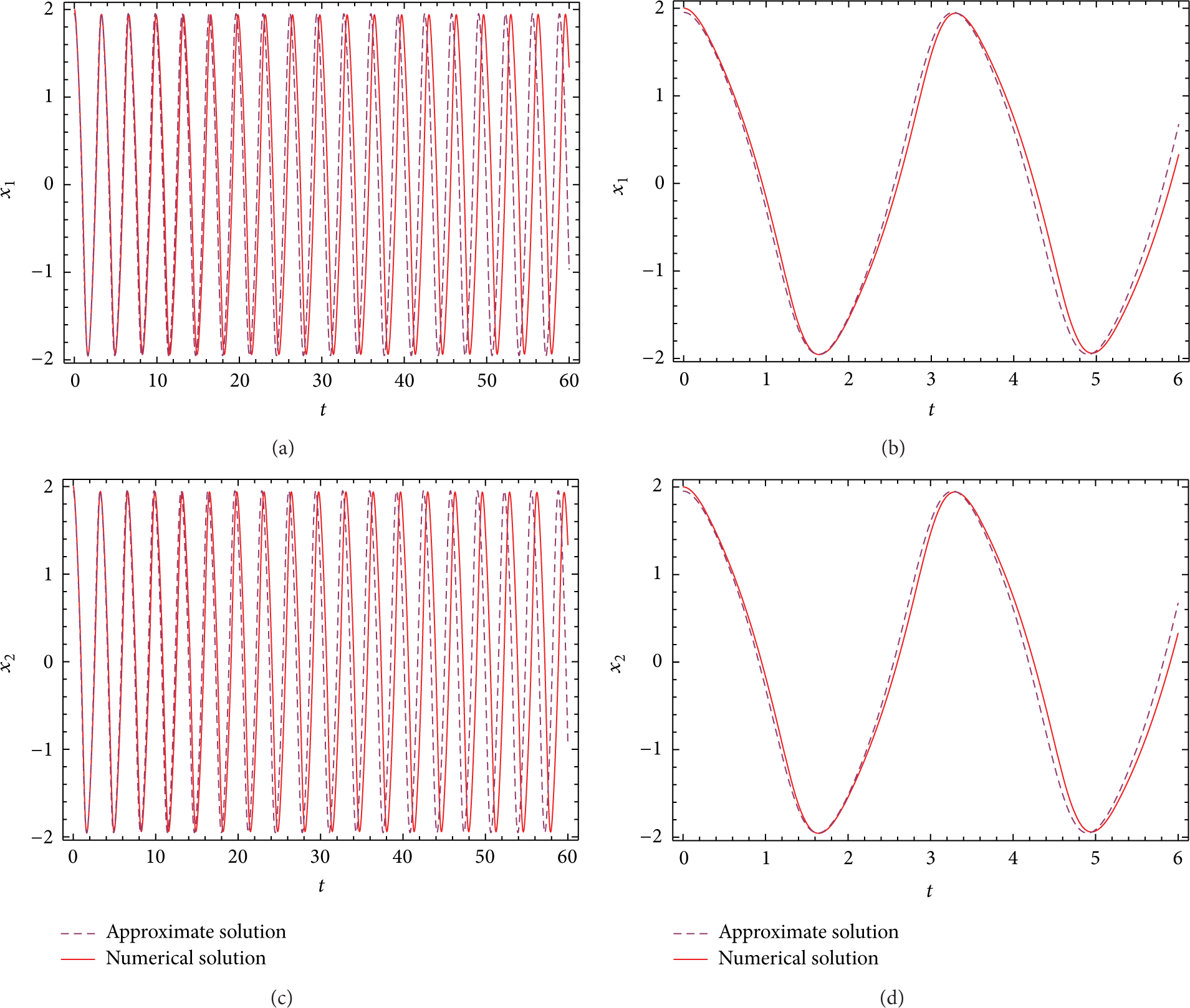
Figures 10 and 11 give the fourth-order analytical approximate phase diagram and time history curve, respectively. As is shown in the figures, fourth-order analytical approximation agrees well with the solution obtained by the numerical integration method. Here the initial conditions that numerical integration method meets are x₁(0) = 2, x₁′(0) = 0, x₂(0) = 2, and x₂′(0) = 0.

Figure 10:

Comparison of the phase portrait curves of the fourth-order approximation with the numerical integration method.

Figure 11:

Comparison of the time history responses of the fourth-order approximation with the numerical integration method.

The fourth-order analytical approximation (x₁(t),x₂(t),ω) that systems (1a) and (1b) satisfy the above initial conditions is

$x_{\mathrm{1}}\left(t\right)=\mathrm{1.84397604}\cos \omega t+\mathrm{0.24306765}\sin \omega t+\mathrm{0.08670996}\cos \mathrm{3}\omega t-\mathrm{0.06706854}\sin \mathrm{3}\omega t-\mathrm{0.00132301}\cos \mathrm{5}\omega t-\mathrm{0.00826489}\sin \mathrm{5}\omega t-\mathrm{0.00057043}\cos \mathrm{7}\omega t-\mathrm{0.00010677}\sin \mathrm{7}\omega t\mathrm{0.00000736}\cos \mathrm{9}\omega t+\mathrm{0.00002331}\sin \mathrm{9}\omega t,$

(31a)

$x_{\mathrm{2}}\left(t\right)=\mathrm{1.84397604}\cos \omega t+\mathrm{0.24306765}\sin \omega t+\mathrm{0.08670996}\cos \mathrm{3}\omega t-\mathrm{0.06706854}\sin \mathrm{3}\omega t-\mathrm{0.00132301}\cos \mathrm{5}\omega t-\mathrm{0.00826489}\sin \mathrm{5}\omega t-\mathrm{0.00057043}\cos \mathrm{7}\omega t-\mathrm{0.00010677}\sin \mathrm{7}\omega t-\mathrm{0.00000736}\cos \mathrm{9}\omega t+\mathrm{0.00002331}\sin \mathrm{9}\omega t,$

(31b)

$\omega =\mathrm{2.50306103}.$

(31c)

4. Four Important Theorems

From the above discussion, when α₁ = α₂ = 1, β₁ = β₂ = 1, and δ₁ = δ₂ = 2, the solution of systems (1a) and (1b) satisfies x₁(t) = x₂(t), and the expressions of x₁(t), x₂(t), and ω will not be influenced by parameters γ₁, γ₂, inspired from the results.

Theorem 1. Assuming α, β, δ, and γ _i (i = 1, 2) are real parameters, x(t) is the solution of van der Pol-Duffing equation $\ddot{x}+\alpha (x^{\mathrm{2}}-\mathrm{1})\dot{x}+\beta x+\delta x^{\mathrm{3}}=\mathrm{0}$ ; then for any γ₁,γ₂ ∈ R, x₁(t) = x₂(t) = x(t) is a solution of system

${\ddot{x}}_{\mathrm{1}}+\alpha \left(x_{\mathrm{1}}^{\mathrm{2}}-\mathrm{1}\right){\dot{x}}_{\mathrm{1}}+\beta x_{\mathrm{1}}+\delta x_{\mathrm{1}}^{\mathrm{3}}+{\gamma }_{\mathrm{1}}\left(x_{\mathrm{1}}^{\mathrm{3}}-x_{\mathrm{2}}^{\mathrm{3}}\right)=\mathrm{0},$

(32a)

${\ddot{x}}_{\mathrm{2}}+\alpha (x_{\mathrm{2}}^{\mathrm{2}}-\mathrm{1}){\dot{x}}_{\mathrm{2}}+\beta x_{\mathrm{2}}+\delta x_{\mathrm{2}}^{\mathrm{3}}+{\gamma }_{\mathrm{2}}(x_{\mathrm{2}}^{\mathrm{3}}-x_{\mathrm{1}}^{\mathrm{3}})=\mathrm{0}.$

(32b)

More generally, we have this theorem.

Theorem 2. Assuming α, β, and δ are real parameters, f _i (i = 1, 2) is real function about x₁ and x₂, and when x₁ = x₂, f₁ = f₂ = 0, x(t) is the solution of van der Pol-Duffing equation $\ddot{x}+\alpha (x^{\mathrm{2}}-\mathrm{1})\dot{x}+\beta x+\delta x^{\mathrm{3}}=\mathrm{0}$ and x₁(t) = x₂(t) = x(t) is a solution of system

${\ddot{x}}_{\mathrm{1}}+\alpha \left(x_{\mathrm{1}}^{\mathrm{2}}-\mathrm{1}\right){\dot{x}}_{\mathrm{1}}+\beta x_{\mathrm{1}}+\delta x_{\mathrm{1}}^{\mathrm{3}}+f_{\mathrm{1}}\left(x_{\mathrm{1}},x_{\mathrm{2}}\right)=\mathrm{0},$

(33a)

${\ddot{x}}_{\mathrm{2}}+\alpha \left(x_{\mathrm{2}}^{\mathrm{2}}-\mathrm{1}\right){\dot{x}}_{\mathrm{2}}+\beta x_{\mathrm{2}}+\delta x_{\mathrm{2}}^{\mathrm{3}}+f_{\mathrm{2}}\left(x_{\mathrm{1}},x_{\mathrm{2}}\right)=\mathrm{0}.$

(33b)

It is easy to prove the above two theorems. Take x₁(t) = x₂(t) = x(t) into the systems (32a), (32b), (33a), and (33b) and the equation is established. Note that we do not have to find all solutions of the systems (32a), (32b), (33a), and (33b). However, these two theorems are of positive significance. This type of MDOF coupled van der Pol-Duffing oscillator can be simplified into a single degree of freedom of the van der Pol-Duffing equation, and then we can obtain a periodic solution.

This thought of translating MDOF into SDOF is applicable in many nonlinear systems. Here we explore another type of MDOF coupled van der Pol-Duffing oscillator by Theorems 3 and 4.

Theorem 3. Assuming α, β, δ, and γ _i (i = 1, 2) are real parameters, x(t) is the solution of van der Pol-Duffing equation $\ddot{x}+\alpha (x^{\mathrm{2}}-\mathrm{1})\dot{x}+\beta x+\delta x^{\mathrm{3}}=\mathrm{0}$ , for any γ₁,γ₂ ∈ R, x₁(t) = x(t), and x₂(t) = − x(t) is a solution of system

${\ddot{x}}_{\mathrm{1}}+\alpha (x_{\mathrm{1}}^{\mathrm{2}}-\mathrm{1}){\dot{x}}_{\mathrm{1}}+\beta x_{\mathrm{1}}+\delta x_{\mathrm{1}}^{\mathrm{3}}+{\gamma }_{\mathrm{1}}(x_{\mathrm{1}}^{\mathrm{3}}+x_{\mathrm{2}}^{\mathrm{3}})=\mathrm{0},$

(34a)

${\ddot{x}}_{\mathrm{2}}+\alpha (x_{\mathrm{2}}^{\mathrm{2}}-\mathrm{1}){\dot{x}}_{\mathrm{2}}+\beta x_{\mathrm{2}}+\delta x_{\mathrm{2}}^{\mathrm{3}}+{\gamma }_{\mathrm{2}}(x_{\mathrm{1}}^{\mathrm{3}}+x_{\mathrm{2}}^{\mathrm{3}})=\mathrm{0}.$

(34b)

As the promotion of Theorem 3, we have Theorem 4.

Theorem 4. Assuming α, β, and δ are real parameters, f _i (i = 1, 2) is real function about x₁ and x₂, and when x₁ = x₂, f₁ = f₂ = 0, x(t) is the solution of van der Pol-Duffing equation $\ddot{x}+\alpha (x^{\mathrm{2}}-\mathrm{1})\dot{x}+\beta x+\delta x^{\mathrm{3}}=\mathrm{0}$ , x₁(t) = x(t), and x₂(t) = − x(t) is a solution of system

${\ddot{x}}_{\mathrm{1}}+\alpha (x_{\mathrm{1}}^{\mathrm{2}}-\mathrm{1}){\dot{x}}_{\mathrm{1}}+\beta x_{\mathrm{1}}+\delta x_{\mathrm{1}}^{\mathrm{3}}+f_{\mathrm{1}}(x_{\mathrm{1}},x_{\mathrm{2}})=\mathrm{0},$

(35a)

${\ddot{x}}_{\mathrm{2}}+\alpha (x_{\mathrm{2}}^{\mathrm{2}}-\mathrm{1}){\dot{x}}_{\mathrm{2}}+\beta x_{\mathrm{2}}+\delta x_{\mathrm{2}}^{\mathrm{3}}+f_{\mathrm{2}}(x_{\mathrm{1}},x_{\mathrm{2}})=\mathrm{0}.$

(35b)

The proofs of Theorems 1 and 2 are exactly the same. Next we combine the HAM to study the application of Theorem 3.

In the system of (34a) and (34b), taking α = 1, β = 1, γ₁ = 5, γ₂ = 6, and δ₁ = δ₂ = 1, by Theorem 3, a periodic solution of the system (x₁(t),x₂(t)) meets x₁(t) = − x₂(t) = x(t), wherein x(t) is the solution of equation $\ddot{x}+(x^{\mathrm{2}}-\mathrm{1})\dot{x}+x+x^{\mathrm{3}}=\mathrm{0}$ . Periodic solution of the equation can be approximated by using HAM. Their thoughts are similar to the previous 2-DOF coupled oscillators solving. The proof is easier, so it is not launched.

We get that the sixth-order homotopy approximate solution (x(t),ω) of the equation $\ddot{x}+(x^{\mathrm{2}}-\mathrm{1})\dot{x}+x+x^{\mathrm{3}}=\mathrm{0}$ which meets the initial conditions x(0) = 2 and x′(0) = 0 is

$x\left(t\right)=\mathrm{1.84645601}\cos \omega t+\mathrm{0.33006051}\sin \omega t+\mathrm{0.09685555}\cos \mathrm{3}\omega t-\mathrm{0.08775593}\sin \mathrm{3}\omega t-\mathrm{0.00340889}\cos \mathrm{5}\omega t-\mathrm{0.01327148}\sin \mathrm{5}\omega t-\mathrm{0.00156607}\cos \mathrm{7}\omega t-\mathrm{0.00028437}\sin \mathrm{7}\omega t-\mathrm{0.00009081}\cos \mathrm{9}\omega t+\mathrm{0.00016068}\sin \mathrm{9}\omega t+\mathrm{0.00001575}\cos \mathrm{11}\omega t+\mathrm{0.00001118}\sin \mathrm{11}\omega t+\mathrm{0.00000033}\cos \mathrm{13}\omega t-\mathrm{0.00000107}\sin \mathrm{13}\omega t,$

(36a)

$\omega =\mathrm{1.89931855}.$

(36b)

The sixth-order homotopy approximate solution (x₁(t),x₂(t),ω) of Theorem 3 which meets the initial conditions x₁(0) = 2, x₁′(0) = 0, x₂(0) = − 2, and x₂′(0) = 0 is

$x_{\mathrm{1}}\left(t\right)=\mathrm{1.84645601}\cos \omega t+\mathrm{0.33006051}\sin \omega t+\mathrm{0.09685555}\cos \mathrm{3}\omega t-\mathrm{0.08775593}\sin \mathrm{3}\omega t-\mathrm{0.00340889}\cos \mathrm{5}\omega t-\mathrm{0.01327148}\sin \mathrm{5}\omega t-\mathrm{0.00156607}\cos \mathrm{7}\omega t-\mathrm{0.00028437}\sin \mathrm{7}\omega t-\mathrm{0.00009081}\cos \mathrm{9}\omega t+\mathrm{0.00016068}\sin \mathrm{9}\omega t+\mathrm{0.00001575}\cos \mathrm{11}\omega t+\mathrm{0.00001118}\sin \mathrm{11}\omega t+\mathrm{0.00000033}\cos \mathrm{13}\omega t-\mathrm{0.00000107}\sin \mathrm{13}\omega t,$

(37a)

$x_{\mathrm{2}}\left(t\right)=-\mathrm{1.84645601}\cos \omega t-\mathrm{0.33006051}\sin \omega t-\mathrm{0.09685555}\cos \mathrm{3}\omega t+\mathrm{0.08775593}\sin \mathrm{3}\omega t+\mathrm{0.00340889}\cos \mathrm{5}\omega t+\mathrm{0.01327148}\sin \mathrm{5}\omega t+\mathrm{0.00156607}\cos \mathrm{7}\omega t+\mathrm{0.00028437}\sin \mathrm{7}\omega t+\mathrm{0.00009081}\cos \mathrm{9}\omega t-\mathrm{0.00016068}\sin \mathrm{9}\omega t-\mathrm{0.00001575}\cos \mathrm{11}\omega t-\mathrm{0.00001118}\sin \mathrm{11}\omega t-\mathrm{0.00000033}\cos \mathrm{13}\omega t+\mathrm{0.00000107}\sin \mathrm{13}\omega t,$

(37b)

$\omega =\mathrm{1.89931855}.$

(37c)

Finally, we establish a comparison between the approximate solutions and the Runge-Kutta solution. Figures 12 and 13 represent a sixth-order approximation of the phase diagram and the time history graph, respectively. Clearly, the homotopy approximate solution is consistent with the Runge-Kutta solution.

Figure 12:

Comparison of the phase portrait curves of the sixth-order approximation with the numerical integration method.

Figure 13:

Comparison of the time history responses of the sixth-order approximation with the numerical integration method.

5. Conclusions

In this paper, we use the HAM to get the approximate solution of a class of coupled van der Pol oscillator. We focused on α₁≠α₂, β₁≠β₂, and γ₁≠γ₂. These three cases discussed 2-DOF coupled van der Pol system periodic solution's approximation problem, fully demonstrating the great potential of the HAM in the kinetic study. HAM is a powerful tool for solving the MDOF nonlinear system, which provides simple and ingenious ways to ensure the convergence of the series solution. It is also effective in dealing with equations without depending on the presence of a small parameter. This method not only can be obtained in any order frequency ω and expressions x₁(t) and x₂(t) but also greatly reduces the amount of the theoretical calculation. By the comparison between homotopy approximate solution and the Runge-Kutta solution, we see that the HAM can effectively deal with such parameters of coupled oscillators, just request the values of some parameters are not too big. To some degree, the proved four theorems simplify the solution of the two types of nonlinear systems. We will consider how to solve the response problem to this kind of system when the gap of parameters is relatively big in the future.

Conflict of Interests

The authors declare that there is no conflict of interests regarding the publication of this paper.