Sage Journals: Discover world-class research

Abstract

We describe the development and application of a robot vision based adaptive algorithm for the quality control of the braided sleeving of high pressure hydraulic pipes. With our approach, we can successfully overcome the limitations, such as low reliability and repeatability of braided quality, which result from the visual observation of the braided pipe surface. The braids to be analyzed come in different dimensions, colors, and braiding densities with different types of errors to be detected, as presented in this paper. Therefore, our machine vision system, consisting of a mathematical algorithm for the automatic adaptation to different types of braids and dimensions of pipes, enables the accurate quality control of braided pipe sleevings and offers the potential to be used in the production of braiding lines of pipes. The principles of the measuring method and the required equipment are given in the paper, also containing the mathematical adaptive algorithm formulation. The paper describes the experiments conducted to verify the accuracy of the algorithm. The developed machine vision adaptive control system was successfully tested and is ready for the implementation in industrial applications, thus eliminating human subjectivity.

1. Introduction

The textile analysis approaches for the rope braiding defect detection are mostly used for the detection of suspicious or defective regions [1]. These detection methods can be based on a statistical analysis or they can use a mathematical model for image comparison. Model based approaches are based on the comparison of 3D models with rope/wire images. Feature extraction from cooccurrence matrices can also be used because the rope structure has certain regularities. The most useful features are linear prediction based features, local binary patterns, cooccurrence features, features based on pattern irregularities, histograms of oriented gradients [2], and so forth. Useful statistical methods for fault detection are also the vector autoregression model [3], hidden Markov model for multiple camera views [4], and the one-class classification with Gaussian processes [5]. Machine vision systems are not very adaptable in comparison to biological systems and are almost always adapted to a specific task [6].

In our case, we consider the quality control process for a pipe with a braided outer layer. Later on, in the production process, the pipe is rubberized and used for high pressure hydraulic systems. We want to develop an adaptive algorithm for the detection of errors potentially appearing on the braided sleeving. The algorithm must have the ability to adapt and detect errors on different diameters, different braided density, and different colors of the braided outer layer. To achieve this goal we must first extract different features from the braided outer layer image, define the position and dimensions of three regions of interest on the layer for error detection, calculate the main value of intensity of all three regions, and determine the width of the tolerance field of region intensity levels that is still acceptable. The errors on the braided layer must be detected as soon as they occur, and action to eliminate them should be undertaken. Otherwise the error will continue and we will get a defective product, which means waste. With these kinds of adaptive algorithms, the machine vision can be automated for use with different products without the need for manual calibration of the machine vision program.

Different approaches and algorithms were used by researchers for defect detection on fabrics, steel wires, and ropes [7 –11]. One of the main approaches of the machine vision inspection is to adjust the algorithm to the inspected material and type of defect we want to detect. Structural defects are detected as irregularities which have a low frequency of occurrence [7]. Humans can detect these irregularities in patterns with excellent results even if they are not trained to do so. There are three main criteria for human defect recognition: tolerance for structural parameters, deviation in their size, orientation and layout, and also the presence of undesired objects [7]. One of the basic approaches for the machine vision fault detection is based on grayscale images with Hough transformation and autocorrelation function [8]. For the detection of foreign fibers of different colors, the researchers sometimes use object feature extraction (color, shape, or texture) which can be achieved by using neural networks for outlier detection [9]. New nondestructive visual approaches are based on a statistical and filter based approach called tonality inspection for color tone defects [10]. The statistical analysis is made with a combination of image histogram properties, local binary patterns, and other statistical solutions. In some cases, the defects must also be classified after the initial detection. This is done by using different methods for classification, based on feature extraction of detected abnormalities (color, location, convexity, principal axes, compactness, variance, and elliptical variance) [11].

2. Braided Outer Layer Properties

As the produced rubber pipes are used for high pressure applications, they must have absolutely no errors on the sleeving. The first step to getting a reinforced rubber pipe is the braiding of the outer layer of a rubber core. After the braiding of the outer layer is complete, the pipe outer layer is rubberized and the core is pulled out to get a high pressure pipe. The braided outer layer is of different dimensions and densities, but the errors are the same (Figure 1).

Figure 1:

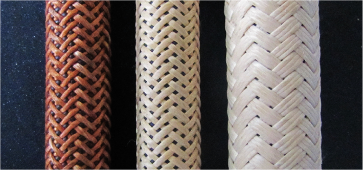
Different types of braiding.

Also, the color of the fibers used for the sleeving varies from white to dark brown. The braided outer layer without errors as seen under IR light is shown in Figure 2.

Figure 2:

Braided outer layer without errors.

The errors during the manufacturing process occur when the fiber tears or gets stuck in the machine. The error persists until the manufacturing process is stopped and all the fibers are installed again. The two different kinds of errors in braiding are knot or loose threads on the outer layer or a missing fiber, as shown in Figure 3. The fault is visible from all directions, so it is possible to detect the fault using only one camera. Also, the pipe is rotating during braiding, and, therefore, the error in the back can be detected even if at a certain moment the fault is not seen by the camera.

Figure 3:

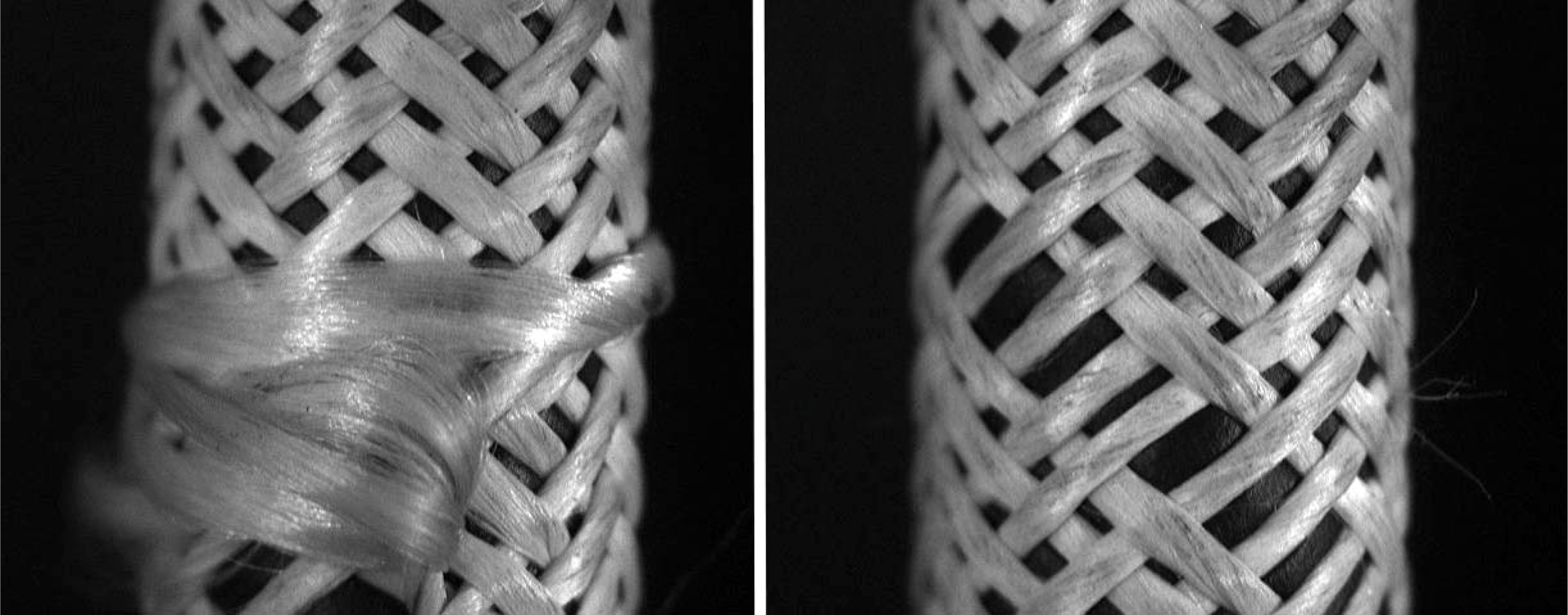
Two types of errors which occur on the braided outer layer.

When the error occurs, the braiding machine must be stopped and reset or the error will persist through the whole manufactured pipe.

3. The Algorithm

The algorithm is implemented using the Matlab programming environment. The program runs on a personal computer and is able to process up to 60 images per second. The final image acquisition speed is decreased so that sufficient image overlapping is achieved. The grayscale digital video camera is positioned in such a way that the rubber pipe runs vertically on the camera image. Figure 4 shows the structure of the algorithm which monitors the braid density, based on the parameters that are gathered at the initialization.

Figure 4:

The algorithm flowchart of the whole control process.

After the image is acquired, it is filtered and converted to a binary image. The braid defect detection is performed on the regions of interest within the filtered image. We only analyze the parts of the image containing the relevant information. Region C covers the middle part of the braid, while the other two regions, A and B, are positioned on the left and on the right side of the braid (Figure 5). The middle region of interest is used to detect the missing threads which are broken off. The left and right regions of interest are used to detect the threads which are hanging loose.

Figure 5:

Error detection areas: C: center area, A: left area, and B: right area.

The initialization steps of our procedure are shown on the left side of the flowchart in Figure 4. The first step is the measuring of the width of the braid. Then, the region of interest of the camera image is selected based on the detected position and width of the braid. In the next step, we determine the average density of the braid. We make sure that the sampled braid density is uniform. Afterwards, we set the tolerance threshold based on the sampled braid density. Once the initialization is complete, the main program starts.

3.1. The Initialization Stage

3.1.1. Width Measurement and Positioning of Regions of Interest

The measuring of the width of the braid and its position is accomplished by detecting the two borders of the braid on the filtered image (Figure 5). We detect the borders as lines using the standard Hough transform [12, 13]. From the positions of the two lines, we determine the distance between the lines and the position of the middle of the braid. We label the left border position in pixels as l_L and the right border position in pixels as l_R.

To detect the width and the position of the regions of interest we first perform Canny edge detection on a binary image since this method has good detection, good localization, and good signal-to-noise ratio. The Canny edge detection algorithm is divided into 4 different steps [13].

Step 1: the image is smoothed with the use of the Gaussian filter to filter out the noise (see (1)), where f_x and f_y represent new intensity values of each pixel, G_x and G_y are gradient elements, and σ is standard deviation:

\begin{matrix} f_{x} = f \cdot G_{x}; G_{x} = \frac{- x}{σ^{2}} \cdot G (x, y), \\ f_{x} = f \cdot G_{y}; G_{y} = \frac{- y}{σ^{2}} \cdot G (x, y) . \end{matrix}

(1)

Step 2: the local gradient approximation ∇f (see (2)) and edge direction α(x,y) are calculated (see (3)):

\nabla f \approx | G_{x} | + | G_{y} |,

(2)

α (x, y) = ta n^{- 1} \cdot (\frac{G_{y}}{G_{x}}) .

(3)

Step 3: the edges are computed with the Sobel edge detection algorithm (see (4)) using a 3 × 3 mask as presented in Table 1 [13]:

\begin{matrix} G_{x} = (z_{7} + 2 z_{8} + z_{9}) - (z_{1} + 2 z_{2} + z_{3}), \\ G_{y} = (z_{3} + 2 z_{6} + z_{9}) - (z_{1} + 2 z_{4} + z_{7}) . \end{matrix}

(4)

Nonmaximum suppression is used to trace along the edges and suppress any pixels that are not considered to be an edge.

Step 4: the last step is performing the edge linking of pixel neighbors.

Table 1:

Pixel indexing of 3 × 3 mask.

z ₁	z ₂	z ₃
z ₄	z ₅	z ₆
z ₇	z ₈	z ₉

Then we use the Hough transform to detect all vertical edges, including those which are tilted up to 20 degrees from the vertical axis. The standard Hough transform is a popular method for the detection of straight lines on images [13]. It can detect lines which appear imperfect or broken. The image is usually preprocessed using an edge detection algorithm.

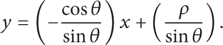
Each line can be represented with two parameters (Figure 6): ρ represents the distance between the origin and the line and θ represents the angle between the horizontal axis and the line (see (5)):

ρ = x \cdot \cos θ + y \cdot \sin θ .

(5)

Parameter θ has a value between −90 and + 90 degrees. A horizontal line θ equals 0 degrees. This normal representation of a line is used for the standard Hough transform instead of the slope-intercept straight line equation, y = kx + n, because parameter k approaches infinity as the line approaches the vertical.

Figure 6:

Rho-theta parameters of a line.

Each straight line can be represented as a point in the rho-theta plane (see (6)):

y = (- \frac{\cos θ}{\sin θ}) x + (\frac{ρ}{\sin θ}) .

(6)

All the lines going through a certain pixel with image coordinates (x_i,y_i) can be represented by

r (θ) = x_{i} \cdot \cos θ + y_{i} \cdot \sin θ .

(7)

Because we want to group points which lie on the same line even though the line is imperfect, we place the (ρ,θ) points into discrete groups by subdividing the rho-theta plane before searching for the intersections.

After both edges of the sleeving are detected, the algorithm automatically determines the width of all three areas according to rubber pipe diameter D which is calculated using l_L and l_R position data (see (8)), where l_L and l_R are the positions of the left and right lines in pixels (Figure 7):

D = l_{R} - l_{L} .

(8)

Distances l_A and l_C are calculated so that l_A is 3 mm wide to avoid false positive detection due to pipe bending. The pipe is rotating during production; therefore a slightly slimmer area C as initially selected can still detect errors on the edges and behind camera view.

Figure 7:

Areas of error detection with distances l_R, l_L, l_A, l_C and D.

3.1.2. Braid Density Evaluation

Before we start to evaluate the braid density, we have to check that there are no errors present during the evaluation of the optimal braid density. We do this by measuring a braid sample. We measure the light intensity of the middle region of interest. We check that the image intensity is uniform in the whole region of interest by dividing the region into three parts in the direction of the movement of the braid. The middle area ratio of white to dark pixels is compared to areas C₁, C₂, and C₃ to determine if there are errors present in the starting phase as shown in Figure 8. This is done by calculating the light intensity I_Ci first (see (9)) and then using the standard deviation calculations (see (10) and (11)). If one of the values differs significantly from the other two (σ < E, where E is the experimentally determined threshold), the braid sample contains a defect and the evaluation has to be repeated with a different sample (I_Ci: area intensity, n_Ci: number of pixels in area C_i, j: index of the pixel, and I(j): pixel brightness (1 or 0)):

I_{C_{i}} = \frac{\sum_{j = 0}^{n_{C_{i}}} I (j)}{n_{C_{i}}},

(9)

I_{C D} = \frac{I_{C_{1}} + I_{C_{2}} + I_{C_{3}}}{3},

(10)

σ = \sqrt{E {(I_{C_{i}} - I_{C D})}^{2}} .

(11)

If the three values are similar, we use the computed baseline light intensity I_CD for error detection in the next steps.

Figure 8:

Areas of error detection for braid density measurement.

3.1.3. Tolerance Threshold Settings

The tolerance threshold of the light intensity of the region of interest is used to determine the size of defects which are considered to be unacceptable. We determine the tolerance threshold by measuring the braid sample and then note the minimum and the maximum as well as the average value. We set the tolerance threshold experimentally to be 10 percent bigger than the biggest difference between the measured and the average values.

We detect errors with the statistical method of averaging the light intensity I_px of each region of interest (see (12)) and compare the result with a preset threshold value ε_dif (see (13)):

I_{mean} = \sum_{region} I_{p x},

(12)

| (I_{mean} - I_{sample}) | > ε_{dif} .

(13)

The threshold value is measured as the average intensity of the rubber pipe sample without defects. If the difference between the measured average intensity of the measured pipe and the average intensity of the sample is bigger than the predefined maximum allowed difference, an error is recognized.

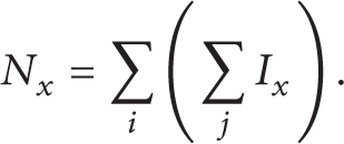
We count the number of all pixels in the region of interest N_x (see (14)):

N_{x} = \sum_{i} (\sum_{j} I_{x}) .

(14)

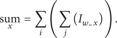
Then we count the number of light pixels of the image in the region of interest sum_x, where x is region A, region B, or region C and I_{w_x} is the number of white pixels in an x region (see (15)) (Figure 7):

\underset{x}{sum} = \sum_{i} (\sum_{j} (I_{w_x})) .

(15)

We also calculate the average intensity I_X: intensity in areas A, B, and C—left, right, and center areas (see (16)). N_x is the number of all pixels in the region of interest:

I_{x} = \frac{{sum}_{x}}{N_{x}} .

(16)

3.1.4. Braid Defect Detection

Whenever the difference between the measured braid density (light intensity of the region of interest) and the density sampled during the initialization is bigger than the tolerance threshold, an error is detected. We use error classifier for each region to determine if the measured average intensity lies within the acceptable limits (see (17)):

\begin{array}{l} f_{C} (I) = {\begin{cases} 1, & (I (C) > 0.7) & (I (C) < 0.62) \\ 0, & otherwise \end{cases} \\ f_{A} (I) = {\begin{cases} 1, & (I (A) > 0.03) \\ 0, & otherwise \end{cases} \\ f_{B} (I) = {\begin{cases} 1, & (I (B) > 0.03) \\ 0, & otherwise . \end{cases} \end{array}

(17)

When the error is detected, the braiding machine would stop and the display would show the message “error detected.”

4. Experimental Setup

For the development and testing of our machine algorithm, we have built an experimental setup (Figure 9) with a pneumatic linear actuator which moves the pipe with the same speed as in the production process. For image acquisition, a grayscale camera with a resolution of 640 × 480 pixels and without an infrared filter is used. To achieve the best possible contrast between the underlying black rubber and the different colors of the pipe the IR LED light source is used. With the use of this light source, even the dark brown outer layer can be reliably detected due to the high contrast with the background. The whole machine is encased in a box (not shown in the figure) which prevents the interference of outside light sources.

Figure 9:

Experimental setup consisting of a grayscale CCD camera (A), an IR LED light source (B), a sample of the braided sleeving (C), and a pneumatic linear actuator (D).

5. Results

The tests were carried out on video recordings that were produced using our experimental setup. We made recording of the braided sleeving with and without defects. The calculation of the appropriate tolerance threshold was performed using a pipe without errors. The intensity level observed in area C had relatively small deviations, which is crucial for an accurate error detection system. The deviation from the norm in the presence of an error was at least two times higher. The intensity level is shown in the graph in Figure 10, where the intensity goes over the tolerance threshold if errors are detected. The graph shows the average intensity levels of each image of the recorded video. Each grayscale image with a resolution of 640 × 480 pixels was processed in 0.12 s on a computer with a processor Intel Core 2 Duo CPU E7400 2.8 GHz 2 GB RAM.

Figure 10:

Graph of light intensity of the three regions of interest during the test run.

In area B, there were no detected errors and the intensity level stayed 0 the whole time. In areas C and A, there were multiple errors detected. Every error was detected multiple times since the captured images of the tested pipe overlapped. In Figure 11, the graph of two different errors of area C on images 278 and 298 is marked as errors Et-278 and Et-298, where Et-z represents the detected error in image z.

Figure 11:

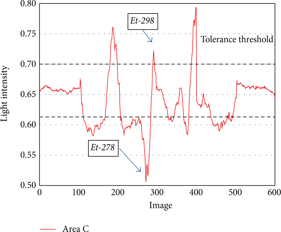
Change in light intensity in Et-278 and Et-298.

The intensity in Et-278 is below the tolerance threshold since the analyzed area consists of more black areas due to a braiding error. In Figure 12, the detected error with a missing fiber is shown.

Figure 12:

Detected missing thread error Et-278 with lower intensity on (a) and the threshold image which is used for the intensity calculation of this error on (b).

The detection algorithm also detects errors which cause an increased intensity level as a result of a knot formation on the pipe surface. An example of such an error is Et-298 and it is shown in Figure 13.

Figure 13:

Error with a knot formation on the surface (a) and the threshold image for intensity calculation on (b).

Error detection in areas A and B is simpler since the error is recognized (present) as soon as the intensity reaches a level higher than 0. In Figure 14, the intensity levels of area A are shown, with Et-295 error highlighted; the graphical representation is shown in Figure 15.

Figure 14:

Changes in light intensity in area A and the first detected error, Et-295.

Figure 15:

Error with a knot formation on the surface, detected in area A (a), and the threshold image for intensity calculation on (b).

6. Conclusions

Computer vision systems are not yet an integral part of braiding machines. In this paper, we propose the use of the adaptive algorithm for fault detection in different braiding with different diameters, density, and color. Adaptive algorithms for error detection in similar production systems can be gained in the same way with the help of future extraction procedures which remove the need for manual settings whenever the different variants of products are being manufactured on the same machines. Our solution is easy to implement and can be reliable if the rubber pipe is well lit and does not move perpendicularly to the direction of the pipe movement. With the use of this adaptive algorithm with a relatively inexpensive CCD camera and controller, we can minimize production losses of high pressure rubber pipes since the braiding stops immediately after the error occurs.

Conflict of Interests

The authors declare that there is no conflict of interests regarding the publication of this paper.

References

Wacker

E.-S.

and Denzler

, “Enhanced anomaly detection in wire ropes by combining structure and appearance,” Pattern Recognition Letters, vol. 34, no. 8, pp. 942–953, 2013.

Platzer

, “On the suitability of different Features for anomaly detection in wire ropes,” in Computer Vision, Imaging and Computer Graphics. Theory and Applications, Communications in Computer and Information Science, pp. 296–308, 2010.

Haase

Wacker

E.-S.

Schukat-Talamazzini

E. G.

, and Denzler

, “Analysis of structural dependencies for the automatic visual inspection of wire ropes,” in Proceedings of the 15th International Workshop on Vision, Modeling and Visualization (VMV '10), pp. 49–56, Siegen, Germany, November 2010.

Platzer

E.-S.

Nägele

Wehking

K.-H.

, and Denzler

, “HMM-based defect localization in wire ropes—a new approach to unusual subsequence recognition,” in Pattern Recognition, vol. 5748 of Lecture Notes in Computer Science, pp. 442–451, Springer, Berlin, Germany, 2009.

Rodner

Wacker

E.-S.

Kemmler

, and Denzler

, “One-class classification for anomaly detection in wire ropes with Gaussian processes in a few lines of code,” in Proceedings of the 12th IAPR Conference on Machine Vision Applications (MVA '11), pp. 219–222, Nara, Japan, June 2011.

Herakovic

, “Computer and machine vision in robot-based assembly,” Journal of Mechanical Engineering, vol. 53, pp. 858–873, 2007.

Chetverikov

, “Structural defects: general approach and application to textile inspection,” in Proceedings of 15th International Conference on Pattern Recognition, Barcelona, Spain, September 2000.

Bakker

Wouters

van Asselt

, “A vision based row detection system for sugar beet,” Computers and Electronics in Agriculture, vol. 60, no. 1, pp. 87–95, 2008.

Yang

, and Wang

, “Classification of foreign fibers in cotton lint using machine vision and multi-class support vector machine,” Computers and Electronics in Agriculture, vol. 74, no. 2, pp. 274–279, 2010.

10.

Xie

and Goon

B. A.

, “Review of recent advances in surface defect detection using texture analysis techniques,” Electronic Letters on Computer Vision and Image Analysis, vol. 7, no. 3, pp. 1–22, 2008.

11.

Iivarinen

and Visa

, “An adaptive texture and shape based defect classification,” Proceedings of the 14th International Conference on Pattern Recognition, vol. 1, pp. 117–122, Brisbane, Australia, 1998.

12.

Asano

and Katoh

, “Variants for the Hough transform for line detection,” Computational Geometry, vol. 6, no. 4, pp. 231–252, 1996.

13.

Gonzalez

R. C.

Woods

R. E.

, and Eddins

S. L.

, Digital Image Processing Using MATLAB, Pearson Prentice-Hall, 2004.

Adaptive Algorithm for the Quality Control of Braided Sleeving

Abstract

1. Introduction

2. Braided Outer Layer Properties

3. The Algorithm

3.1. The Initialization Stage

3.1.1. Width Measurement and Positioning of Regions of Interest

3.1.2. Braid Density Evaluation

3.1.3. Tolerance Threshold Settings

3.1.4. Braid Defect Detection

4. Experimental Setup

5. Results

6. Conclusions

Conflict of Interests

References