Test of Robot Distance Error and Compensation of Kinematic Full Parameters

Abstract

In order to improve the positioning accuracy of robots in the workspace, the maximum cube of robots is solved according to ISO 9283:1998 standard. In addition, in order to efficiently test and identify the kinematic parameters of robots, a mapping from robot's distance error onto kinematic parameter errors is presented based on Hayati's modified D-H model. Then, by analyzing the condition number of distance error matrix, it is concluded that parameter d _i can be deleted when parameter β _i is added in the joint of the modified model. Furthermore, by analyzing the relationship among the parameters of the distance error model, it is found that the deletion of some unidentified kinematic parameters may not result in the accuracy decrease of kinematic error model. Finally, some compensation experiments of the proposed model without unidentified kinematic parameters are carried out by using a laser tracker system. The results show that the proposed method effectively reduces the distance error and greatly improves the positioning accuracy of robots.

1. Introduction

The absolute accuracy of robot is always lower than its repeatability accuracy because the actual kinematics parameters are not identical to the nominal kinematics parameters. It must compensate the kinematic parameters error. In accordance with Roth et al. [1], the main sources of robot positioning errors can be divided into two main groups: geometrical kinematic parameter errors (link lengths, assembling errors, etc.) and nongeometrical ones (compliant errors, measurement errors, environment factors, control errors, friction, backlash, wear, etc.). The main source of the robot inaccuracy is the geometrical kinematic parameter errors because the external forces/torques applied to the end-effector are relatively small. There are open-loop methods and closed-loop methods on robot calibration [2]. By attaching the end-effector to the ground and forming a closed kinematic chain, closed-loop methods calibration used joint angle sensing only, without any external measuring equipment. At present, the most popular calibration methods are the so-called open-loop methods that enable any kind of measurement devices to obtain the pose of the end-effector.

Hollerbach and Wampler [2] proposed a kinematic differential error model mapping the robot error and the kinematic parameters. When a joint is nearly parallel to its neighboring joint, a small error may result in a large error of the robot end-effector. As the small error cannot be modeled by the D-H model, Hayati Samad [3] put forward a modified D-H model which introduced the β _i parameter between two y axes. Stone et al. [4] established the S model. The model includes 6 parameters for each joint and helps to obtain the actual robot kinematic parameters through identifying the axis errors. Zhuang and Roth [5] utilized a camera model to calibrate robot via a modified CPC model. Although the methods of Stone et al. and Zhuang et al. both help to obtain satisfactory results, they use a new kinematic model instead of the D-H kinematic model, which is generally employed. Röning and Korzun [6] calibrated D-H kinematic parameters by using the distance error. Gong et al. [7] proposed a self-calibration method using distance error. Ha [8] calibrates Hayati modified D-H kinematic model which has five parameters in each joint using the distance (relative position) error. All these abovementioned methods achieved satisfactory experimental results. Moreover, in order to accurately calibrate robots, many optimization methods were proposed, such as the particle swarm optimization method proposed by Alıcı et al. [9] and the genetic programming method presented by Dolinsky et al. [10]. These optimization methods are effective in improving robot accuracy. However, more experimental data are needed during the application of the optimization methods, which may result in great computation complexity. Because some kinematic parameter errors cannot be identified, Meggiolaro and Dubowsky [11] proposed identifiable robot error parameters and presented a method to eliminate the redundant parameters in the process of robot calibration.

In the existing calibration methods, the robot workspace where the robot operates is not sufficiently considered. Many methods have been proposed to optimize the pose selection during robot calibration [12–14], but they all use the calibration methods considering the large space that a robot can attach. However, in this space, there are many positions at which the robot is never used or is seldom utilized. Furthermore, all the methods use the least square method (LSM) to calibrate the error parameters. To weigh the error parameters, the LSM will distribute the weight affecting the error of measurement points including the points that are seldom utilized. These points are not necessary because they reduce the weights of useful space points.

To address these problems the remainder of this paper is organized as follows. Firstly, the maximum cube in the workspace of robots is solved according to ISO 9283:1998 standard (Figure 5). Secondly, a mapping from robot's distance error onto kinematic parameter errors is presented based on Hayati's modified D-H model. It should be mentioned here that these error sources may be either independent or correlated, but, in practice, they are usually treated sequentially, assuming that they are statistically independent [15]. Thirdly, this paper analyzes the D-H parameters and it deletes unidentifiable ones. Finally, the robot kinematic model is compensated by using the identified kinematic parameter errors, thus successfully improving the robot accuracy.

2. Robot Distance Error Testing

2.1. Coordinate Transformation of Robot Coordinate and Laser Tracker System

Figure 1 is the schematic drawing of a robot and the corresponding measurement instrument Leica laser tracker system (LTS). For the robot, the base frame is {0}, the robot end-effector frame is {e}, and the measurement frame is {M}. As shown in Figure 1, a₁, a₂, and a₃ are D-H parameters and are used to solve the maximum cube in the later part of this paper.

Figure 1:

Schematic drawing of robot and LTS.

Here, we use homogeneous coordinates to describe the robot kinematic model and a 4 × 4 matrix to describe the robot pose. The first 3 rows of the fourth column in this matrix describe the robot position. The orientation and position of frame {e} to the frame $\left\{0\right\}{}^0{\mathbf{T}}_e$ can be described as follows:

${}^0{\mathbf{T}}_e=\left(\begin{array}{cccc}{n}_{ex}& o_{ex}& a_{ex}& p_{ex}\\ n_{ey}& o_{ey}& a_{ey}& p_{ey}\\ n_{ez}& o_{ez}& a_{ez}& p_{ez}\\ \mathrm{0}& \mathrm{0}& \mathrm{0}& \mathrm{1}\end{array}\right).$

(1)

The robot end-effector position is ${\mathbf{p}}_e={\left[\begin{array}{ccc}{p}_{ex}& p_{ey}& p_{ez}\end{array}\right]}^T$ .

The homogeneous coordinate matrix of the robot endpoint, namely, ${}^0{\mathbf{T}}_n$ that describes the orientation and position of endpoint frame {n} to the frame {0}, is

${}^0{\mathbf{T}}_n=\left(\begin{array}{cccc}{n}_{nx}& o_{nx}& a_{nx}& p_{nx}\\ n_{ny}& o_{ny}& a_{ny}& p_{ny}\\ n_{nz}& o_{nz}& a_{nz}& p_{nz}\\ \mathrm{0}& \mathrm{0}& \mathrm{0}& \mathrm{1}\end{array}\right).$

(2)

The robot endpoint position is ${\mathbf{p}}_n={\left[\begin{array}{ccc}{p}_{nx}& p_{ny}& p_{nz}\end{array}\right]}^T$ .

According to ISO 9283:1998 standard, the accuracy measurement of a robot is to test the robot's end distance, so that p _n should be known. As ${}^0{\mathbf{T}}_e$ can be obtained by the LTS directly and ${}^n{\mathbf{T}}_e$ can be indirectly calculated, p _n can be calculated by the following formulas:

${}^0{\mathbf{T}}_e={}^0{\mathbf{T}}_n{}^n{\mathbf{T}}_e,$

(3)

${}^0{\mathbf{T}}_n={}^0{\mathbf{T}}_e{\left({}^n{\mathbf{T}}_e\right)}^{-\mathrm{1}}.$

(4)

2.2. Maximum Cube of Robot Workspace

Here, we use the “Manipulating industrial robots: Performance criteria and related test methods” in ISO 9283:1998 to measure the robot distance accuracy. The maximum cube with side lengths of 250, 400, 630, and 1000 mm should be used. The centre of the selected cube is shown in Figure 2.

Figure 2:

Testing cubic of location in accordance to standard.

To obtain the maximum cube, we should

1. calculate a maximum cube in the workspace;

2. place the centre of the selected cube in the centre of a cube with the maximum allowable cube;

3. acquire 5 testing points: P₁, P₂, P₃, P₄, and P₅ in the standard cube.

For experimental robot, the range of each joint rotation is shown in Table 1.

Table 1:

Range of robot rotation (deg).

Joint	Minimum (deg)	Maximum (deg)
θ1	−170	170
θ2	−175	30
θ3	−155	80
θ4	−180	180
θ5	−130	130
θ6	−360	360

The maximum rotation angle of joint 2 is max⁡(θ₂) = 80°.

The robot link parameters are shown in Table 2.

Table 2:

Link parameters (mm).

Parameters	a 1	a 2	a 3	d 4
Value	170	560	153	634

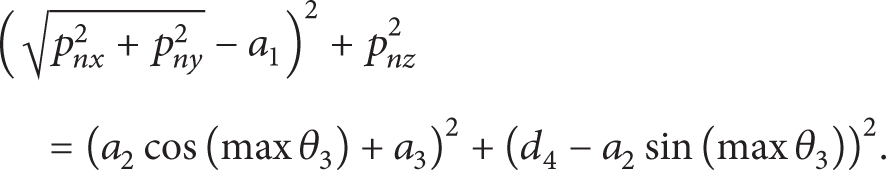
When the robot endpoint and link 2 are both in the same line, the robot can achieve its maximum radius from which the outer boundary can be obtained. According to the relation of space geometric rotation, the robot rotates along joints θ₁ and θ₂ to reach the point (p _nx ,p _ny ,p _nz ) on the outer boundary surface (see Figure 3), and

${\left(\sqrt{p_{nx}^{\mathrm{2}}+p_{ny}^{\mathrm{2}}}-a_{\mathrm{1}}\right)}^{\mathrm{2}}+p_{nz}^{\mathrm{2}}={\left(\sqrt{a_{\mathrm{3}}^{\mathrm{2}}+d_{\mathrm{4}}^{\mathrm{2}}}+a_{\mathrm{2}}\right)}^{\mathrm{2}}.$

(5)

Figure 3:

The outer boundary surface.

In addition, point (p _nx ,p _ny ,p _nz ) on the inner boundary surface (see Figure 4) must satisfy

${\left(\sqrt{p_{nx}^{\mathrm{2}}+p_{ny}^{\mathrm{2}}}-a_{\mathrm{1}}\right)}^{\mathrm{2}}+p_{nz}^{\mathrm{2}}={\left(a_{\mathrm{2}}\cos \left(\max {\theta }_{\mathrm{3}}\right)+a_{\mathrm{3}}\right)}^{\mathrm{2}}+{\left(d_{\mathrm{4}}-a_{\mathrm{2}}\sin \left(\max {\theta }_{\mathrm{3}}\right)\right)}^{\mathrm{2}}.$

(6)

By solving formula ((6)), there comes

$\sqrt{p_{nx}^{\mathrm{2}}+p_{ny}^{\mathrm{2}}}\ge \mathrm{230.3835}.$

(7)

Then, we establish the objective function as the longest side of s.

Figure 4:

The inner boundary surface.

Figure 5:

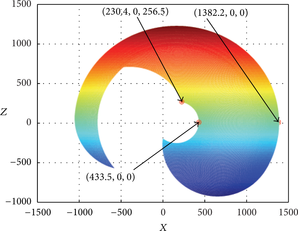
The maximum workspace of robot.

Constraints are as follows:

1. outer curve constraints: C₄ should be on the outer boundary surface or below the inner surface;

2. inner curve constraints: F should be on the inner boundary surface or on the inner surface;

3. $\sqrt{a^{\mathrm{2}}+{\mathrm{0}}^{\mathrm{2}}}=a\ge \mathrm{230.3835}$ .

Let C₄(a + s,s/2,c + s) and F(a,0,c) in the constrains (1)~(3). The optimal value of the objective function is 678.4706, and variable values s, a, and c are solved to get 679.4706, 433.4938, and 0, respectively.

Consequently, the maximum cube in workspace is 680 mm per side, and the centre of the selected cube is the centre of the maximum cube, that is, (a + s/2,0,c + s/2). Thus, the centre point is (773, 0, 340) and the cube is shown in Figure 6.

Figure 6:

The maximum cube in workspace.

2.3. Experiments of Testing Robot Distance Error by LTS

The experiments were carried out on the robot GSK08 made by Guangzhou CNC Equipment Company, China. LTS Leica AT901 with a precision of ±10 μm + 5 μm/m was used as the measurement apparatus. It consists of a laser tracker, an AT controller, a reflector, and a processor equipped with software package PolyWorks v11. The measured target is a reflector assembled to the end-effector by a fixture specially designed for robot measurement. When a laser line is emitted by the tracker and is reflected by the reflector, the position in 3-dimension of the reflector is calculated by the tracking system. As the orientation measurement algorithm is the same as the position one, only the position measurement was performed in this experiment (see Figure 7).

Figure 7:

Measurement of robot distance error by laser tracker system.

3. Kinematic Parameter Errors Model for Distance Error

3.1. Robot Kinematic Model

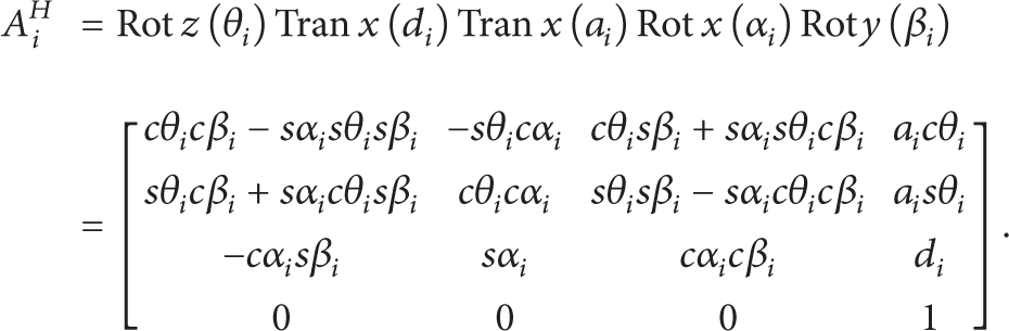
The Denavit-Hartenberg (D-H) homogeneous transformation matrix is widely applied to the robot kinematic analysis, as shown in the following formula:

$A_i=\text{Rot}\hspace{0.17em}z\left({\theta }_i\right)\text{Tran}\hspace{0.17em}x\left(d_i\right)\text{Tran}\hspace{0.17em}x\left(a_i\right)\text{Rot}\hspace{0.17em}x\left({\alpha }_i\right).$

(8)

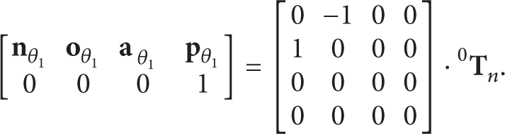
If z_{i − 1} and z_{i − 1} are nearly parallel, a modified Hayati D-H homogeneous transformation matrix is used; that is,

$\begin{array}{c}{A}_i^H=\text{Rot}\hspace{0.17em}z\left({\theta }_i\right)\text{Tran}\hspace{0.17em}x\left(d_i\right)\text{Tran}\hspace{0.17em}x\left(a_i\right)\text{Rot}\hspace{0.17em}x\left({\alpha }_i\right)\text{Rot}y\left({\beta }_i\right)\\ =\left[\begin{array}{cccc}c{\theta }_{i}c{\beta }_i-s{\alpha }_{i}s{\theta }_{i}s{\beta }_i& -s{\theta }_{i}c{\alpha }_i& c{\theta }_{i}s{\beta }_i+s{\alpha }_{i}s{\theta }_{i}c{\beta }_i& a_{i}c{\theta }_i\\ s{\theta }_{i}c{\beta }_i+s{\alpha }_{i}c{\theta }_{i}s{\beta }_i& c{\theta }_{i}c{\alpha }_i& s{\theta }_{i}s{\beta }_i-s{\alpha }_{i}c{\theta }_{i}c{\beta }_i& a_{i}s{\theta }_i\\ -c{\alpha }_{i}s{\beta }_i& s{\alpha }_i& c{\alpha }_{i}c{\beta }_i& d_i\\ 0& 0& 0& 1\end{array}\right].\end{array}$

(9)

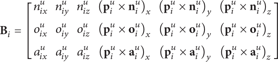
3.2. Robot Joint Kinematic Error Parameters Model

Setting P to be the robot endpoint pose relative to the base frame including position and orientation, it is supposed that the base frame coincides with the world frame. Let R be a 3 × 3 rotation matrix about the angle ϕ, and p is the endpoint position vector; there is

$\mathbf{P}=\mathbf{g}\left(k\right)={}^0{\mathbf{T}}_n=\left[\begin{array}{cc}\mathbf{R}& \mathbf{p}\\ \mathrm{0}& \mathrm{1}\end{array}\right].$

(10)

Instead of the orientation matrix R , it is convenient to represent the orientation by vector of ϕ_α, ϕ_β, and ϕ_γ. P = [ϕ_α,ϕ_β,ϕ_γ,p _x ,p _y ,p _z ], ϕ_α, ϕ_β, and ϕ_γ are Euler angle. It is the same to robot position p , and p _x , p _y , and p _z are the robot position.

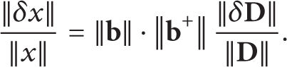
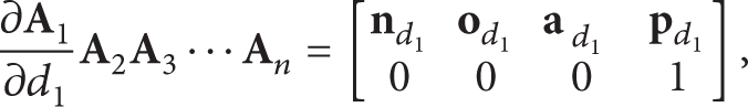
Let the robot endpoint position be p = g(k), and k is robot full kinematic parameter: k = [θ₁ a₁ d₁ α₁ β₁ ⋯ θ _i  a _i  d _i  α _i  β _i  ⋯ θ _n  a _n  d _n  α _n  β _n ].

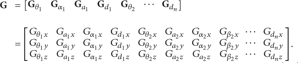
For each joint, the mapping from the matrix A _i deviation onto the differential change Δ _i is

$d{A}_i=A_i^a-A_i=A_i{\Delta }_i,$

(11)

where A _i ^a is actual matrix of A _i and Δ _i is

${\Delta }_i={\left(A_i\right)}^{-\mathrm{1}}d{A}_i=\left[\begin{array}{cccc}\mathrm{0}& -\delta z_i& \delta y_i& d{x}_i\\ \delta z_i& \mathrm{0}& -\delta x_i& d{y}_i\\ -\delta y_i& \delta x_i& \mathrm{0}& d{z}_i\\ \mathrm{0}& \mathrm{0}& \mathrm{0}& \mathrm{0}\end{array}\right].$

(12)

The differential of matrix A _i is

$d{A}_i=\frac{\partial A_i}{\partial {\theta }_i}\delta {\theta }_i+\frac{\partial A_i}{\partial d_i}\delta d_i+\frac{\partial A_i}{\partial a_i}\delta a_i+\frac{\partial A_i}{\partial {\alpha }_i}\delta {\alpha }_i+\frac{\partial A_i}{\partial {\beta }_i}\delta {\beta }_i.$

(13)

The partial derivatives of matrix A _i to the kinematic parameters are

$\begin{array}{c}\frac{\partial {\mathbf{A}}_i}{\partial {\theta }_i}=\left[\begin{array}{cccc}-s{\theta }_i& -c{\theta }_{i}c{\alpha }_i& c{\theta }_{i}s{\alpha }_i& -a_{i}s{\theta }_i\\ c{\theta }_i& -s{\theta }_{i}c{\alpha }_i& s{\theta }_{i}s{\alpha }_i& a_{i}c{\theta }_i\\ \mathrm{0}& \mathrm{0}& \mathrm{0}& \mathrm{0}\\ \mathrm{0}& \mathrm{0}& \mathrm{0}& \mathrm{0}\end{array}\right],\\ \frac{\partial {\mathbf{A}}_i}{\partial {\alpha }_i}=\left[\begin{array}{cccc}\mathrm{0}& s{\theta }_{i}s{\alpha }_i& s{\theta }_{i}c{\alpha }_i& \mathrm{0}\\ \mathrm{0}& -c{\theta }_{i}s{\alpha }_i& -c{\theta }_{i}c{\alpha }_i& \mathrm{0}\\ \mathrm{0}& c{\alpha }_i& -s{\alpha }_i& \mathrm{0}\\ \mathrm{0}& \mathrm{0}& \mathrm{0}& \mathrm{0}\end{array}\right],\\ \frac{\partial {\mathbf{A}}_i}{\partial a_i}=\left[\begin{array}{cccc}\mathrm{0}& \mathrm{0}& \mathrm{0}& s{\theta }_i\\ \mathrm{0}& \mathrm{0}& \mathrm{0}& c{\theta }_i\\ \mathrm{0}& \mathrm{0}& \mathrm{0}& \mathrm{0}\\ \mathrm{0}& \mathrm{0}& \mathrm{0}& \mathrm{0}\end{array}\right],\hspace{1em}\hspace{1em}\frac{\partial {\mathbf{A}}_i}{\partial d_i}=\left[\begin{array}{cccc}\mathrm{0}& \mathrm{0}& \mathrm{0}& \mathrm{0}\\ \mathrm{0}& \mathrm{0}& \mathrm{0}& \mathrm{0}\\ \mathrm{0}& \mathrm{0}& \mathrm{0}& \mathrm{1}\\ \mathrm{0}& \mathrm{0}& \mathrm{0}& \mathrm{0}\end{array}\right].\end{array}$

(14)

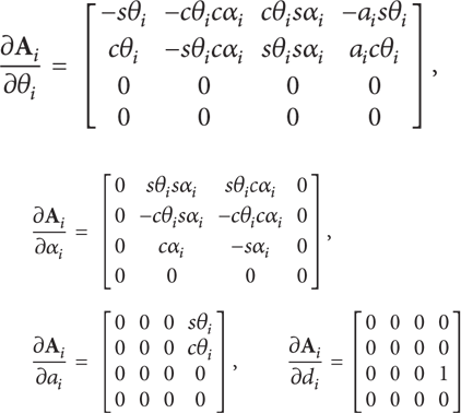
When the neighbor joints are nearly parallel, d _i = 0, and the partial derivative of matrix A _i to kinematic parameter β _i is

$\frac{\partial {\mathbf{A}}_i}{\partial {\beta }_i}=\left[\begin{array}{cccc}-s{\theta }_{i}s{\alpha }_i& \mathrm{0}& c{\theta }_i& \mathrm{0}\\ c{\theta }_{i}s{\alpha }_i& \mathrm{0}& s{\theta }_i& \mathrm{0}\\ -c{\alpha }_i& \mathrm{0}& \mathrm{0}& \mathrm{0}\\ \mathrm{0}& \mathrm{0}& \mathrm{0}& \mathrm{0}\end{array}\right],$

(15)

${\Delta }_i={\left({\mathbf{A}}_i^n\right)}^{-\mathrm{1}}d{\mathbf{A}}_i=\left[\begin{array}{cccc}\mathrm{0}& -(s{\beta }_i\delta {\alpha }_i+c{\alpha }_{i}c{\beta }_i\delta {\theta }_i)& s{\alpha }_i\delta {\theta }_i+\delta {\beta }_i& c{\beta }_i\delta a_i+a_{i}s{\alpha }_{i}s{\beta }_i\delta {\theta }_i-c{\alpha }_{i}s{\beta }_i\delta d_i\\ s{\beta }_i\delta {\alpha }_i+c{\alpha }_{i}c{\beta }_i\delta {\theta }_i& \mathrm{0}& -(c{\beta }_i\delta {\alpha }_i-c{\alpha }_{i}s{\beta }_i\delta {\theta }_i)& a_{i}c{\alpha }_i\delta {\theta }_i+s{\alpha }_i\delta d_i\\ -(s{\alpha }_i\delta {\theta }_i+\delta {\beta }_i)& c{\beta }_i\delta {\alpha }_i-c{\alpha }_{i}s{\beta }_i\delta {\theta }_i& \mathrm{0}& s{\beta }_i\delta a_i-a_{i}s{\alpha }_{i}c{\beta }_i\delta {\theta }_i+c{\alpha }_{i}c{\beta }_i\delta d_i\\ \mathrm{0}& \mathrm{0}& \mathrm{0}& \mathrm{0}\end{array}\right],$

(16)

$e_i={\left[\begin{array}{cccccc}d{x}_i& d{y}_i& d{z}_i& \delta x_i& \delta y_i& \delta z_i\end{array}\right]}^T$

(17)

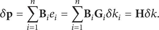
Each kinematic parameter error of robot joint is mapped onto the joint differential error e _i as formula ((18)):

$e_i=\left[\begin{array}{ccccc}{a}_{i}s{\alpha }_{i}s{\beta }_i& -\text{c}{\alpha }_{i}s{\beta }_i& c{\beta }_i& \mathrm{0}& \mathrm{0}\\ a_{i}c{\alpha }_i& s{\alpha }_i& \mathrm{0}& \mathrm{0}& \mathrm{0}\\ -a_{i}s{\alpha }_{i}c{\beta }_i& c{\alpha }_{i}c{\beta }_i& s{\beta }_i& \mathrm{0}& \mathrm{0}\\ -c{\alpha }_{i}s{\beta }_i& 0& 0& c{\beta }_i& 0\\ s{\alpha }_i& 0& 0& 0& 1\\ c{\alpha }_{i}c{\beta }_i& 0& 0& s{\beta }_i& 0\end{array}\right]\left[\begin{array}{c}\delta {\theta }_i\\ \delta d_i\\ \delta a_i\\ \delta {\alpha }_i\\ \delta {\beta }_i\end{array}\right]={\mathbf{G}}_i\delta k_i,$

(18)

where k _i is a certain joint kinematic parameter. When joint i is parallel to joint i + 1, $k_i={\left[\begin{array}{ccccc}{\theta }_i& a_i& d_i& {\alpha }_i& {\beta }_i\end{array}\right]}^T$ and its kinematic parameter error $\delta k_i={\left[\begin{array}{ccccc}\delta {\theta }_i& \delta a_i& \delta d_i& \delta {\alpha }_i& \delta {\beta }_i\end{array}\right]}^T$ ; otherwise, $k_i={\left[\begin{array}{cccc}{\theta }_i& a_i& d_i& {\alpha }_i\end{array}\right]}^T$ and its kinematic parameter error $\delta k_i={\left[\begin{array}{cccc}\delta {\theta }_i& \delta a_i& \delta d_i& {\alpha }_i\end{array}\right]}^T$ . G _i is the matrix of robot error coefficients matrix.

The actual endpoint error is obtained by the measurement apparatus. However, a certain joint error e _i is relative to the base frame. It needs to transform error e _i from the base frame to the endpoint frame. Hence, matrix ${}^n{U}_i$ , a transformation matrix from joint i frameto the robot endpoint frame, is introduced, and

${}^n{U}_i=A_{i+\mathrm{1}}{A}_{i+\mathrm{2}}\cdots A_n=\left[\begin{array}{cccc}{\mathbf{n}}_i^u& {\mathbf{o}}_i^u& {\mathbf{a}}_i^u& {\mathbf{p}}_i^u\\ \mathrm{0}& \mathrm{0}& \mathrm{0}& \mathrm{1}\end{array}\right].$

(19)

Here, the robot orientation error is not discussed due to the space limit. B _i can transform a certain joint differential error e _i to the robot endpoint frame, and

${\mathbf{B}}_i=\left[\begin{array}{cccccc}{n}_{ix}^u& n_{iy}^u& n_{iz}^u& {\left({\mathbf{p}}_i^u\times {\mathbf{n}}_i^u\right)}_x& {\left({\mathbf{p}}_i^u\times {\mathbf{n}}_i^u\right)}_y& {\left({\mathbf{p}}_i^u\times {\mathbf{n}}_i^u\right)}_z\\ o_{ix}^u& o_{iy}^u& o_{iz}^u& {\left({\mathbf{p}}_i^u\times {\mathbf{o}}_i^u\right)}_x& {\left({\mathbf{p}}_i^u\times {\mathbf{o}}_i^u\right)}_y& {\left({\mathbf{p}}_i^u\times {\mathbf{o}}_i^u\right)}_z\\ a_{ix}^u& a_{iy}^u& a_{iz}^u& {\left({\mathbf{p}}_i^u\times {\mathbf{a}}_i^u\right)}_x& {\left({\mathbf{p}}_i^u\times {\mathbf{a}}_i^u\right)}_y& {\left({\mathbf{p}}_i^u\times {\mathbf{a}}_i^u\right)}_z\end{array}\right].$

(20)

δ P is the endpoint error between the robot nominal pose and the actual pose. It can be measured by LTS:

$\delta \mathbf{p}={\displaystyle \sum }_{i=\mathrm{1}}^n{\mathbf{B}}_i{e}_i={\displaystyle \sum }_{i=\mathrm{1}}^n{\mathbf{B}}_i{\mathbf{G}}_i\delta k_i=\mathbf{H}\delta k.$

(21)

For a certain point j in the workspace, its position error is

$\delta {\mathbf{p}}_j={\displaystyle \sum }_{i=\mathrm{1}}^n{\mathbf{B}}_{ij}{e}_{ij}={\displaystyle \sum }_{i=\mathrm{1}}^n{\mathbf{B}}_{ij}{\mathbf{G}}_{ij}\delta k_i={\mathbf{H}}_j\delta k.$

(22)

3.3. Robot Distance Error Model

The robot positions of two arbitrary points j and j + 1 are, respectively, p _j and p_{j + 1}.

If we move the robot in the base frame, the laser tracker can track two points j and j + 1 in the measurement frame. The positions of these two points are described by

${\mathbf{p}}_{j,j+\mathrm{1}}={\mathbf{p}}_j-{\mathbf{p}}_{j+\mathrm{1}}.$

(23)

The commander distance of these two points is

$D_{j,j+\mathrm{1}}^c={\mathbf{p}}_j^c-{\mathbf{p}}_{j+\mathrm{1}}^c.$

(24)

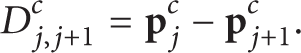
And the actual distance between these two points is

$D_{j,j+\mathrm{1}}^a={\mathbf{p}}_j^a-{\mathbf{p}}_{j+\mathrm{1}}^a.$

(25)

The relationship between the robot commander distance and the actual distance is shown in Figure 8.

Figure 8:

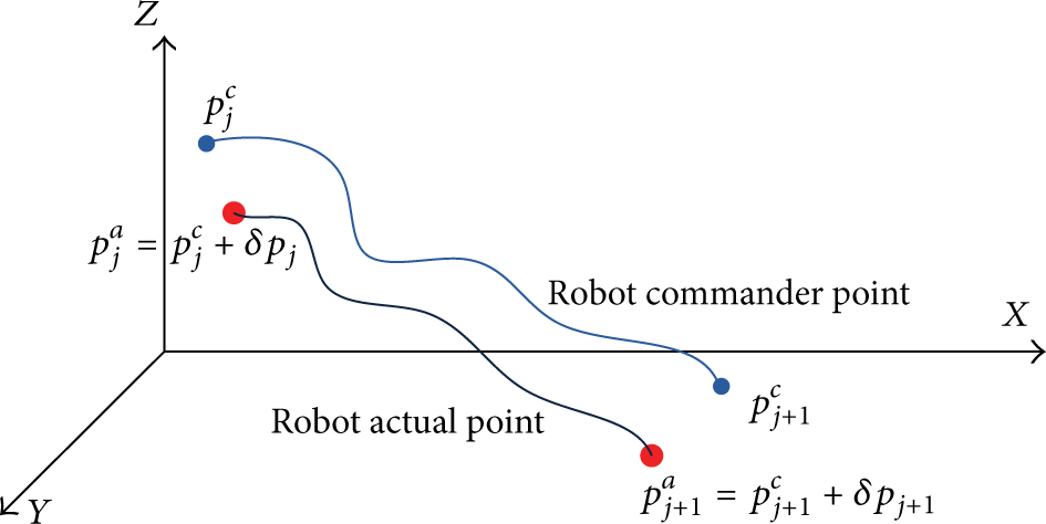
Relationship between commander distance and actual distance.

From formula ((18)), one can obtain δp _j as a certain point error: δp _j = H _j δk, δp_{j + 1} = H_{j + 1}δk.

δp _j is the error of point j between the commander distance and the measured one, and

$\delta p_j=p_j^a-p_j^c={\mathbf{H}}_j\delta k.$

(26)

δp_{j + 1} is the error of point j + 1 between the commander distance and the measured one, and

$\delta p_{j+\mathrm{1}}=p_{j+\mathrm{1}}^a-p_{j+\mathrm{1}}^c={\mathbf{H}}_{j+\mathrm{1}}\delta k.$

(27)

D_{j,j + 1} ^a is the actual distance between points j and j + 1; that is,

$D_{j,j+\mathrm{1}}^a=\Vert p_j^a-p_{j+\mathrm{1}}^a\Vert .$

(28)

The square of Euclidian actual distance is

${\Vert D_{j,j+\mathrm{1}}^a\Vert }^{\mathrm{2}}={\Vert {\mathbf{p}}_j^a-{\mathbf{p}}_{j+\mathrm{1}}^a\Vert }^{\mathrm{2}}={\Vert {\mathbf{p}}_j^c+{\mathbf{H}}_j\delta k-\left({\mathbf{p}}_{j+\mathrm{1}}^c+{\mathbf{H}}_{j+\mathrm{1}}\delta k\right)\Vert }^{\mathrm{2}}={\Vert D_{j,j+\mathrm{1}}^c+\left({\mathbf{H}}_j-{\mathbf{H}}_{j+\mathrm{1}}\right)\delta k\Vert }^{\mathrm{2}}.$

(29)

Supposing that

$\begin{array}{c}{\mathbf{D}}_j={\Vert {\mathbf{D}}_{j,j+\mathrm{1}}^a\Vert }^{\mathrm{2}}-{\Vert {\mathbf{D}}_{j,j+\mathrm{1}}^c\Vert }^{\mathrm{2}},\\ x=\delta k,\\ {\mathbf{b}}_j=\mathrm{2}{\left(D_{j,j+\mathrm{1}}^c\right)}^T{}^T\left({\mathbf{H}}_j-{\mathbf{H}}_{j+\mathrm{1}}\right)\delta k,\end{array}$

(30)

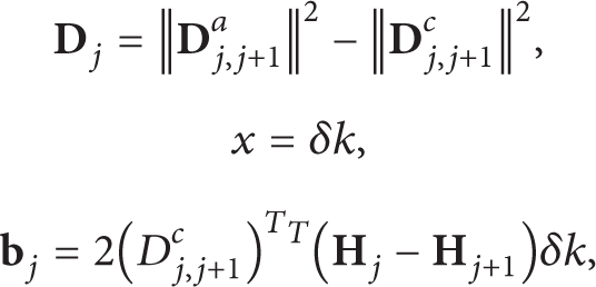
there is

${\mathbf{D}}_j={\mathbf{b}}_{j}x.$

(31)

By using the least square method (LSM), it obtains

$\text{minimize:}{\displaystyle \sum }_{j=\mathrm{1}}^m{\Vert {\mathit{D}}_j-{\mathit{b}}_{j}x\Vert }_{\mathrm{2}}^{\mathrm{2}},\phantom{\text{minm}:\text{ze}}{\displaystyle \sum }_{j=\mathrm{1}}^m\left({\mathbf{b}}_j^T{\mathbf{b}}_j\right)x={\displaystyle \sum }_{j=\mathrm{1}}^m\left({\mathbf{b}}_j^T{\mathbf{D}}_j\right),$

(32)

$\mathbf{b}=\left[\begin{array}{cccc}{b}_{\mathrm{1}}& b_{\mathrm{2}}& \cdots & b_m\end{array}\right],\hspace{1em}\mathbf{D}=\left[\begin{array}{cccc}{D}_{\mathrm{1}}& D_{\mathrm{2}}& \cdots & D_m\end{array}\right].$

(33)

m is the number of measurement:

$x={\left({\mathbf{b}}^T\mathbf{b}\right)}^{-\mathrm{1}}{\mathbf{b}}^T\mathbf{D}.$

(34)

Thus, the estimated value ○ can be obtained.

4. Kinematic Parameter Errors Identification

4.1. Modified D-H Parameters Numerical Analysis

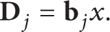
The condition number of a full-rank matrix b ⁺ is given by

$\mathbf{b}\left(x+\delta x\right)=\mathbf{D}+\delta \mathbf{D}.$

(35)

Supposing that b₊ = (b _T b)⁻¹b _T and δx = b₊ δD, by taking the (Euclidean) norms of both sides, we have

$\Vert \delta x\Vert \le \Vert {\mathbf{b}}^{+}\Vert \Vert \delta \mathbf{D}\Vert .$

(36)

According to the inequality ‖D‖ = ‖b₊ x‖ ≤ ‖b₊ ‖·‖x‖, ‖·‖ is the (Euclidean) norms; there comes

$\frac{\Vert \delta x\Vert }{\Vert x\Vert }=\Vert \mathbf{b}\Vert ·\Vert {\mathbf{b}}^{+}\Vert \frac{\Vert \delta \mathbf{D}\Vert }{\Vert \mathbf{D}\Vert }.$

(37)

cond(b) = ‖b‖·‖b₊ ‖ is the condition number of matrix b , and

$\text{con}{\text{d}}_{\mathrm{2}}\left(\mathbf{b}\right)={\Vert \mathbf{b}\Vert }_{\mathrm{2}}·{\Vert {\mathbf{b}}^{+}\Vert }_{\mathrm{2}}.$

(38)

Cond₂( b ⁺) is the 2-norm condition number of matrix b ⁺.

Large condition number may result in a system with high sensitivity, which means that even small changes of D and b ⁺ may result in huge changes in the solution x . In this paper, we compute the condition number to know whether it is necessary to delete kinematic parameter d _i when it adds kinematic parameter β _i . Cond₂( b ) is of an order of magnitude of 10¹⁷ if parameter d _i is not deleted and is of an order of magnitude of 10⁴ if d _i is deleted. So that d _i should be deleted during the computation of the kinematic parameters.

4.2. Unidentified Kinematic Parameter Errors of Distance Error

The robot endpoint deviation relative to the base frame is $d{}^0{\mathbf{T}}_n$ . From the base frame to the endpoint frame, it can get

$d{}^0{\mathbf{T}}_n={\displaystyle \sum }_{i=\mathrm{1}}^n{\mathbf{A}}_{\mathrm{1}}\cdots \frac{\partial {\mathbf{A}}_i}{\partial {\theta }_i}{\mathbf{A}}_{i+\mathrm{1}}\cdots {\mathbf{A}}_n\delta {\theta }_i+{\displaystyle \sum }_{i=\mathrm{1}}^n{\mathbf{A}}_{\mathrm{1}}\cdots \frac{\partial {\mathbf{A}}_i}{\partial {\alpha }_i}{\mathbf{A}}_{i+\mathrm{1}}\cdots {\mathbf{A}}_n\delta {\alpha }_i+{\displaystyle \sum }_{i=\mathrm{1}}^n{\mathbf{A}}_{\mathrm{1}}\cdots \frac{\partial {\mathbf{A}}_i}{\partial a_i}{\mathbf{A}}_{i+\mathrm{1}}\cdots {\mathbf{A}}_n\delta a_i+{\displaystyle \sum }_{i=\mathrm{1}}^n{\mathbf{A}}_{\mathrm{1}}\cdots \frac{\partial {\mathbf{A}}_i}{\partial d_i}{\mathbf{A}}_{i+\mathrm{1}}\cdots {\mathbf{A}}_n\delta d_i.$

(39)

The matrix G is

$\begin{array}{c}\mathbf{G}=\left[\begin{array}{ccccccc}{\mathbf{G}}_{{\theta }_{\mathrm{1}}}& {\mathbf{G}}_{{\alpha }_{\mathrm{1}}}& {\mathbf{G}}_{a_{\mathrm{1}}}& {\mathbf{G}}_{d_{\mathrm{1}}}& {\mathbf{G}}_{{\theta }_{\mathrm{2}}}& \cdots & {\mathbf{G}}_{d_n}\end{array}\right]\\ =\left[\begin{array}{cccccccccc}{G}_{{\theta }_{\mathrm{1}}x}& G_{a_{\mathrm{1}}x}& G_{{\alpha }_{\mathrm{1}}x}& G_{d_{\mathrm{1}}x}& G_{{\theta }_{\mathrm{2}}x}& G_{a_{\mathrm{2}}x}& G_{{\alpha }_{\mathrm{2}}x}& G_{{\beta }_{\mathrm{2}}x}& \cdots & G_{d_{n}x}\\ G_{{\theta }_{\mathrm{1}}y}& G_{a_{\mathrm{1}}y}& G_{{\alpha }_{\mathrm{1}}y}& G_{d_{\mathrm{1}}y}& G_{{\theta }_{\mathrm{2}}y}& G_{a_{\mathrm{2}}y}& G_{{\alpha }_{\mathrm{2}}y}& G_{{\beta }_{\mathrm{2}}y}& \cdots & G_{d_{n}y}\\ G_{{\theta }_{\mathrm{1}}z}& G_{a_{\mathrm{1}}z}& G_{{\alpha }_{\mathrm{1}}z}& G_{d_{\mathrm{1}}z}& G_{{\theta }_{\mathrm{2}}z}& G_{a_{\mathrm{2}}z}& G_{a_{\mathrm{2}}z}& G_{{\beta }_{\mathrm{2}}z}& \cdots & G_{d_{n}z}\end{array}\right].\end{array}$

(40)

According to the Meggiolaro method, G_d1 and G_θ1 can be solved by

${\mathbf{G}}_{d_{\mathrm{1}}}=\frac{\partial {\mathbf{A}}_{\mathrm{1}}}{\partial d_{\mathrm{1}}}{\mathbf{A}}_{\mathrm{2}}{\mathbf{A}}_{\mathrm{3}}\cdots {\mathbf{A}}_n,$

(41)

${\mathbf{G}}_{{\theta }_{\mathrm{1}}}=\frac{\partial {\mathbf{A}}_{\mathrm{1}}}{\partial {\theta }_{\mathrm{1}}}{\mathbf{A}}_{\mathrm{2}}{\mathbf{A}}_{\mathrm{3}}\cdots {\mathbf{A}}_n,$

(42)

where ∂A₁/∂d₁ and ∂A₁/∂θ₁ can be solved according to

$\frac{\partial {\mathbf{A}}_{\mathrm{1}}}{\partial d_{\mathrm{1}}}{\mathbf{A}}_{\mathrm{2}}{\mathbf{A}}_{\mathrm{3}}\cdots {\mathbf{A}}_n=\left[\begin{array}{cccc}{\mathbf{n}}_{d_{\mathrm{1}}}& {\mathbf{o}}_{d_{\mathrm{1}}}& \mathbf{a}{}_{d_{\mathrm{1}}}{}^{\mathrm{\hspace{0.17em}\hspace{0.17em}}}\mathrm{\hspace{0.17em}\hspace{0.17em}}& {\mathbf{p}}_{d_{\mathrm{1}}}\\ \mathrm{0}& \mathrm{0}& \mathrm{0}& \mathrm{1}\end{array}\right],\hspace{1em}\hspace{1em}\hspace{1em}\hspace{1em}$

(43)

$\frac{\partial {\mathbf{A}}_{\mathrm{1}}}{\partial {\theta }_{\mathrm{1}}}{\mathbf{A}}_{\mathrm{2}}\cdots {\mathbf{A}}_n=\left[\begin{array}{cccc}{\mathbf{n}}_{{\theta }_{\mathrm{1}}}& {\mathbf{o}}_{{\theta }_{\mathrm{1}}}& \mathbf{a}{}_{{\theta }_{\mathrm{1}}}{}^{\mathrm{\hspace{0.17em}\hspace{0.17em}}}\mathrm{\hspace{0.17em}\hspace{0.17em}}& {\mathbf{p}}_{{\theta }_{\mathrm{1}}}\\ \mathrm{0}& \mathrm{0}& \mathrm{0}& \mathrm{1}\end{array}\right]=\left[\begin{array}{cccc}\mathrm{0}& -\mathrm{1}& \mathrm{0}& \mathrm{0}\\ \mathrm{1}& \mathrm{0}& \mathrm{0}& \mathrm{0}\\ \mathrm{0}& \mathrm{0}& \mathrm{0}& \mathrm{0}\\ \mathrm{0}& \mathrm{0}& \mathrm{0}& \mathrm{0}\end{array}\right]·\left({\mathbf{A}}_{\mathrm{1}}{\mathbf{A}}_{\mathrm{2}}\cdots {\mathbf{A}}_n\right).$

(44)

Therefore,

$\left[\begin{array}{cccc}{\mathbf{n}}_{{\theta }_{\mathrm{1}}}& {\mathbf{o}}_{{\theta }_{\mathrm{1}}}& \mathbf{a}{}_{{\theta }_{\mathrm{1}}}{}^{\mathrm{\hspace{0.17em}\hspace{0.17em}}}\mathrm{\hspace{0.17em}\hspace{0.17em}}& {\mathbf{p}}_{{\theta }_{\mathrm{1}}}\\ \mathrm{0}& \mathrm{0}& \mathrm{0}& \mathrm{1}\end{array}\right]=\left[\begin{array}{cccc}\mathrm{0}& -\mathrm{1}& \mathrm{0}& \mathrm{0}\\ \mathrm{1}& \mathrm{0}& \mathrm{0}& \mathrm{0}\\ \mathrm{0}& \mathrm{0}& \mathrm{0}& \mathrm{0}\\ \mathrm{0}& \mathrm{0}& \mathrm{0}& \mathrm{0}\end{array}\right]·{}^0{\mathbf{T}}_n.$

(45)

It can be obtained that ${\mathbf{p}}_{{\theta }_{\mathrm{1}}}={\left[\begin{array}{ccc}-p_{ny}& p_{nx}& \mathrm{0}\end{array}\right]}^T$ , and, furthermore, ${\mathbf{H}}_{d_{\mathrm{1}}}^{}={\mathbf{H}}_{{\theta }_{\mathrm{1}}}^{}=\mathbf{0}$ , which means that d₁ and θ₁ are both unidentified error parameters.

As measuring instruments need no identification, we can obtain the identifiable parameters listed in Table 3.

Table 3:

Identifiable parameters for distance error.

Joint	1	2	3	4	5
A 1	—	—	δa1	δα1	—
A 2	δθ2	—	δa2	δα2	δβ2
A 3	δθ3	δd3	δa3	δα3	—
A 4	δθ4	δd4	δa4	δα4	—
A 5	δθ5	δd5	δa5	δα5	—
A 6	δθ6	δd6	δa6	δα6	—

4.3. Directly Solve the Transformation between the Robot Endpoint and the LTS Reflector

As the installation errors of LTS reflector are not the robot error, a method for error separation should be employed.

As shown in Figure 9, if only joint 6 rotates and other joints are locked, a circle can be obtained. The LTS can capture a rotation axis and the center of this circle (Figure 10). Here, we suppose this axis to be z axis of the robot endpoint frame. Then, rotating joint 5 only and locking other joints, the LTS can capture the y axis of the robot endpoint coordinates. Moreover, the x axis can be obtained based on the right hand rule. Thus, the reflector coordinate values in the endpoint frame can be successfully obtained.

Figure 9:

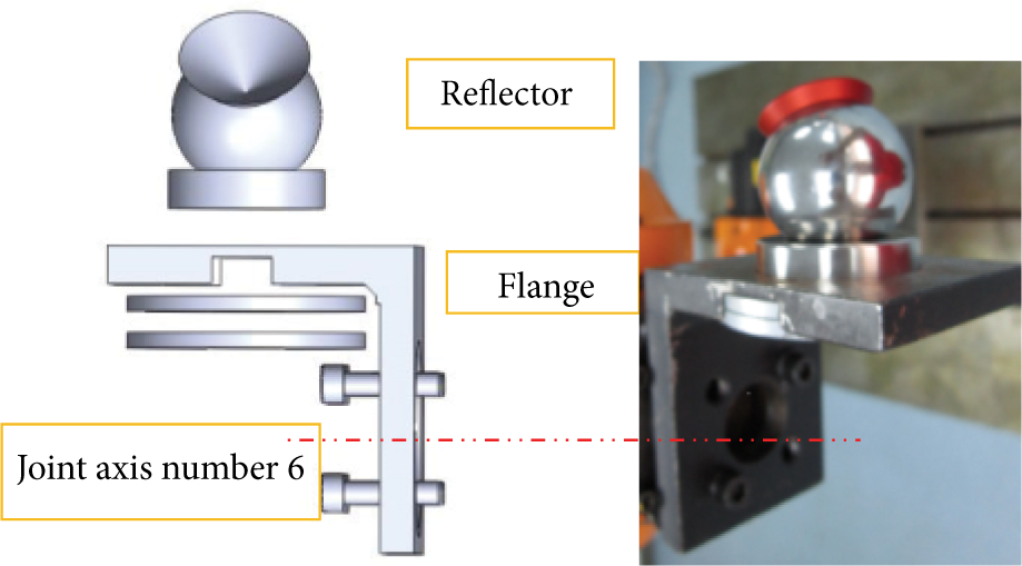
Installation errors of LTS reflector.

Figure 10:

Measuring flange frame by single axis rotation.

5. Experiments of Kinematic Parameter Errors Identification

According to formula ${\mathbf{H}}_{d_{\mathrm{1}}}^{}={\mathbf{H}}_{{\theta }_{\mathrm{1}}}^{}=\mathbf{0}$ , the unidentified parameters of the robot can be deleted and the identified error parameters of the robot can be solved.

If the identified kinematic parameter errors of the robot are obtained, the robot kinematic parameters can be compensated and the statistical indexes after compensation can be obtained for fitting points, as listed in Tables 4 and 5.

Table 4:

Kinematic parameters after compensation.

Joint	θ i /deg	d i /mm	a i /mm	α i /deg	β i /deg
A 1	—	—	169.073710	−89.768265	—
A 2	0.394345	—	560.283258	−0.027072	0.082953
A 3	−0.109999	5.105655	153.959881	−90.469331	—
A 4	1.209951	634.156485	2.454763	91.210896	—
A 5	−0.382655	1.714099	−0.461477	−92.101344	—
A 6	—	151.707698	−2.225226	—	—

Table 5:

Statistical index after compensation for fitting points.

Distance error	Max. error	Absolute mean	Standard deviation
Before compensation (mm)	6.165478	2.722397	2.370663
After compensation (mm)	0.167276	0.045829	0.058326

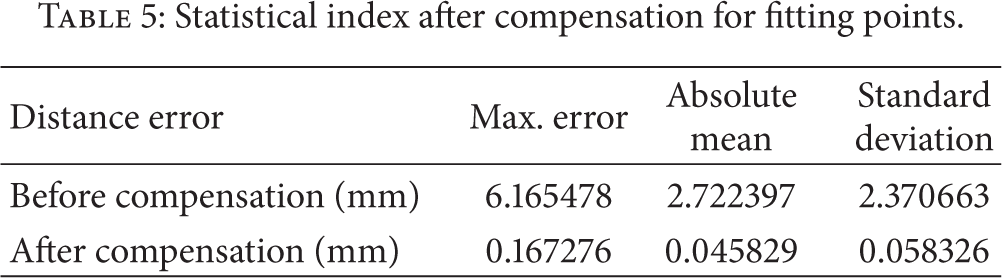
Figure 11 shows the error comparison of fitting points, from which it is found that the robot distance accuracy improves by 98.32% and the standard deviation decreases by 97.54% for fitting points.

Figure 11:

Error comparison of fitting points.

Some other points are selected to test the effectiveness of the compensation, and the results are shown in Figure 12.

Figure 12:

Error comparison of testing points.

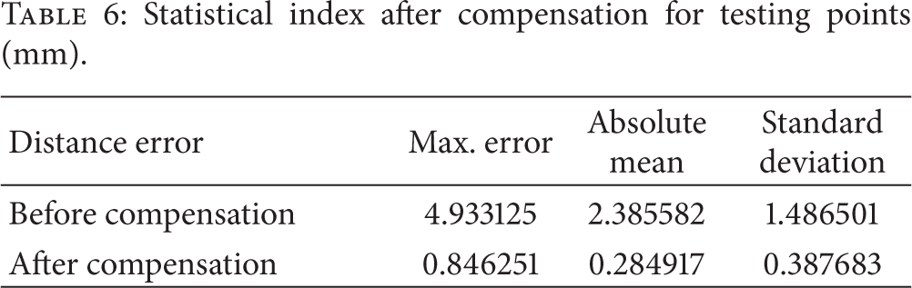
Table 6 lists the statistical indexes after the compensation for testing points, from which it is found that the robot distance accuracy improves by 88.06% and the standard deviation decreases by 73.92% for testing points. This absolute mean is the actual accuracy for robot.

Table 6:

Statistical index after compensation for testing points (mm).

Distance error	Max. error	Absolute mean	Standard deviation
Before compensation	4.933125	2.385582	1.486501
After compensation	0.846251	0.284917	0.387683

6. Conclusion

In the test of robot's distance error, the distribution of points in the whole space may reduce the accuracy of the robot in the workspace. In order to solve this problem, the maximum cube of robots is solved according to ISO 9283:1998 standard. In addition, a mapping from robot's distance error onto kinematic parameter errors is presented based on Hayati's modified D-H model. Then, by analyzing the condition number of distance error matrix, it is concluded that parameter d _i can be deleted when parameter β _i is added in the joint of the modified model. Furthermore, by analyzing the distance error matrix, a new kinematic parameter model deleting unidentified kinematic parameters is established. Finally, some compensation experiments are carried out by using a laser tracker system. The results show that the proposed method is effective and that it helps to reduce the robot endpoint error by 73.9%. The next work is to deal with robot's attitude error and the corresponding compensation method.

Conflict of Interests

The authors declare that there is no conflict of interests regarding the publication of this paper.